Discrete Element Numerical Simulation of the Effect of River Ice Porosity on Impact Force at Bridge Abutments

Abstract

In spring, the river ice melts to a certain extent and cracks to form drift ice and impact force on the bridge abutments; the river ice, due to the impact of ablation, has an internal formation of different porosities, and the level of porosity affects the mechanical properties of the river ice, so that the impact force generated by the river ice is also different. In this paper, the Heihe–Blagoveshchensk Amur River Bridge abutment is the object of river ice impact, and the discrete element method (DEM) is employed to analyze the impact process and impact force on the abutment by numerical simulation of the melting river ice. The damage characteristics of the ice rows with different ice speeds, ice thicknesses, and porosity, and the time curve of the impact force are obtained. It is found that the maximum impact force of river ice on the abutment decreases nonlinearly with the increase in river ice porosity; the peak contact force occurs with a lag time, and the damage is gradually concentrated in the vicinity of the area in direct contact with the abutment. In this paper, according to the simulation results, the relationship between river ice porosity and the maximum impact force on the bridge abutment, as well as the time parameters, is obtained by fitting, and the power loading model of the bridge abutment impacted by the river ice is established, which provides a basis for the reasonable calculation of the impact force of the ablated river ice at bridge abutments.

1. Introduction

Every spring, as temperatures rise, the ice in rivers begins to melt. Under the action of water flow, the ablated river ice cracks and rushes along the river channel, which produces a huge impact on the hydraulic structures, such as bridge piers, that impede the flow of river ice, seriously threatening the safety and stability of the structures [1]. Therefore, an in-depth study of the impact effect of ablating river ice on bridge piers is crucial for ensuring the safe and reliable operation of bridges in regions characterized by low temperatures.

For the problem of structure–ice interaction, relevant research has been carried out by scholars [2,3,4]. Withalm [5] developed an innovative model that enhances the Matlock model, specifically focusing on ice-induced vibrations. The model revealed that the average ice force generated on the structure as well as the rupture frequency of ice mainly depends on the ice’s own parameters. Based on the actual form and structural data of a prototype bridge pier, and based on the contact–collision theory and nonlinear finite element analysis theory, Xufeng Zhang [6] thoroughly investigated the effects of ice strength, elastic modulus, and ice thickness on the maximum ice force of streaming ice with the help of LS-DYNA. The simulation results compellingly demonstrate that the impact force shows an increasing trend as the strength, elastic modulus, and thickness increase. Lianzhen Zhang [7] conducted a study on the collision process between river ice and a bridge pier using LS-DYNA. The results of the simulation indicate that the maximum value of the ice force over time initially increases as the speed of the river ice rises. However, after reaching a certain point, this value begins to decrease with further increases in river ice speed. Tuhkuri [8] performed numerical simulations of ice–structure interactions using the discrete element method (DEM) and verified its unique advantages in characterizing the non-homogeneity of ice materials and dynamic damage processes.

In summary, the current studies on the interaction between structures and ice [9,10] mainly focus on the mechanical characterization of frozen ice [11,12,13,14], while insufficient attention has been paid to the impact effect of porous ice during the ablation period. During spring ablation, changes in the internal porosity of the ice significantly affect its mechanical properties—the dense ice structure formed in winter gradually evolves into a porous medium containing gas bubbles and microcracks [15]. Existing impact studies mostly treat ice as a homogeneous material [16,17], neglecting the effect of porosity, a key parameter, on impact loading. This simplification may lead to the deviation of ice load prediction at bridge abutments, which in turn affects the reliability of the ice-resistant design of bridges in cold regions.

This paper adopts the discrete element method to carry out the simulation of the pore ice impact process, taking the piers of the Heihe–Blagoveshchensk Amur River Bridge as the research object, systematically simulating the impact process under different ice speeds, ice thickness, and porosity conditions, and focusing on revealing the quantitative relationship between the porosity and the peak value of the impact force. The research results will be the first time an ice load dynamic model has been established considering the porosity parameter, which will directly serve bridge engineering practices in cold regions: on the one hand, it can provide refined load inputs for the anti-icing design of bridge piers, avoiding the risk of misestimation of load caused by neglecting the porosity effect in the traditional method; on the other hand, it can provide theoretical support for the safety assessment of existing bridges and effectively improve the safety of bridges operating in high latitude areas during the spring flood season, by revealing the dynamic evolution law of ice load during the melting period. The study is aimed at improving the operational safety of bridges in high-latitude areas during the spring flood season.

2. Materials and Methods

2.1. Discrete Elemental Computational Modeling of River Ice

The DEM treats each particle as an independent unit, and simulates the motion and interaction of the particles by calculating the combined force, acceleration, velocity, and displacement of each unit, and thus has a significant advantage in simulating the behavior of discontinuous and complex materials as well as multibody interactions [18,19,20]. This method can take into account the influence of the internal microstructure of the ice (e.g., porosity) on the macroscopic mechanical behavior [21], which better captures the non-homogeneous nature of ice as well as the complex dynamic behavior of the impact process. The DEM simulates how materials behave by modeling particle contact. Some of the more common contact models are linear contact models, Hertz–Mindlin contact models, point bond contact models, parallel bond contact models, smooth joint contact models, flat joint contact models, hysteresis damping contact models [22], rolling resistance contact models, and Burger’s contact models [23].

Ice is a crystal structure composed of water molecules arranged in an orderly manner, in which the water molecules are connected to each other through hydrogen bonding, forming an architecture that is both broad and strong. In the numerical simulation carried out in this paper by the DEM, the parallel bonded contact model is employed, which is able to realize the simulation of the role of hydrogen bonding torque transfer between crystalline particles, and it is highly suitable for simulating the mechanical behavior of ice materials.

The parallel bond contact model is illustrated in Figure 1. When the stress on the river ice surpasses its tensile strength, bonding bonds in the model will be destroyed, leading to the failure of the bonding between the particle units, thus simulating the fracture behavior of the river ice.

The contact force $F_c$ and contact moment $M_c$ for the parallel bond contact model are given by the following:

$$F_c=F^l+F^d+\overline{F}$$

(1)

$$M_c=\overline{M}$$

(2)

where $F^l$ is the linear contact force, $F^d$ is the damping force, $\overline{F}$ is the parallel bond force, and $\overline{M}$ is the parallel bond moment.

Parallel bond forces $\overline{F}$ can be divided into normal contact forces ${\overline{F}}_n$ and tangential contact forces ${\overline{F}}_s$; parallel bond moment $\overline{M}$ can be divided into torque ${\overline{M}}_t$ and bending moment ${\overline{M}}_b$ as follows:

$$\Delta {\overline{F}}_n=k_{n}A\Delta U_n$$

(3)

$$\Delta {\overline{F}}_s=-k_{s}A\Delta U_s$$

(4)

$$\Delta {\overline{M}}_t=-k_{s}J\Delta {\theta }_t$$

(5)

$$\Delta {\overline{M}}_b=-k_{n}I\Delta {\theta }_s$$

(6)

where $\Delta {\overline{F}}_n$, $\Delta {\overline{F}}_s$, $\Delta {\overline{M}}_t$, $\Delta {\overline{M}}_b$ are the increment of ${\overline{F}}_n$, ${\overline{F}}_s$, ${\overline{M}}_t$, ${\overline{M}}_b$; $k_n$, $k_s$ are the normal contact stiffness and tangential contact stiffness; $\Delta U_n$, $\Delta U_s$, ${\theta }_t$, ${\theta }_s$ are the normal displacement increment, tangential displacement increment, relative torsion increment and relative bending increment.

$A$, $I$ and $J$ are the area, moment of inertia, and polar moment of inertia, respectively.

$$A=\pi R^2$$

(7)

$$I={\displaystyle \frac{1}{4}}\pi R^2$$

(8)

$$J={\displaystyle \frac{1}{2}}\pi R^4$$

(9)

$$R=\min (R_1+R_2)$$

(10)

where $R$ is the contact radius; $R_1$ is the equivalent radius of piece1; $R_2$ is the equivalent radius of piece2.

The maximum normal stress on the parallel bonded bond is given by the following:

$${\sigma }_t={\displaystyle \frac{{\overline{F}}_n}{A}}+{\displaystyle \frac{\left|{\overline{M}}_b\right|R}{I}}$$

(11)

The maximum tangential stress on the parallel bonded bond is given by the following:

$$\tau ={\displaystyle \frac{{\overline{F}}_s}{A}}+{\displaystyle \frac{\left|{\overline{M}}_b\right|R}{J}}$$

(12)

Tensile damage occurs when the contact is subjected to normal stress that exceeds the normal tensile strength of the bond, and shear damage occurs when the tangential stress exceeds the tangential bond strength of the bond.

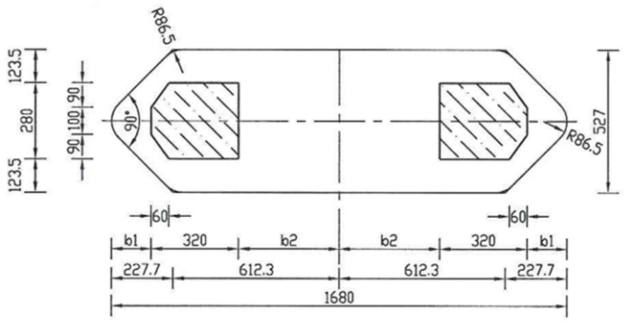
2.2. Overview of the Abutment Project

The project of the Heihe–Blagoveshchensk Amur River Bridge started from Changfatun, Heihe City, Heilongjiang Province, and is located in Kanykurgan Village, Blagoveshchensk City, Russia. As the first steel–concrete combination girder low-tower cable-stayed bridge built in a high-latitude, cold region, the Heihe–Blagoveshchensk Amur River Bridge faces severe ice conditions every spring during the ice flow period. The China–Russia Heilongjiang Bridge piers use a solid pier cross-section for the flat hexagonal, a pier width of 16.8 m, a pier thickness of 5.27 m, and the pier to meet the ice for the tip of the typical tip-type ice-breaking prisms, with an angle of about 90°. The Heihe–Blagoveshchensk Amur River Bridge pier cross-section is shown in Figure 2.

2.3. Discrete Elemental Model of River Ice

In this paper, PFC 5.0 software is utilized to conduct numerical simulations of discrete river ice elements. The discrete element model of river ice is composed of generated particles, and the length of the simulated ice row is 40 m and the width is 30 m. The particles are randomly distributed, with the particle radius of the ice row ranging from 0.3 to 0.48 m, the stacking of the internal particles is determined by the random seed number, and the density of the particles is 980 kg/m³. The fine-scale mechanical parameters were calibrated using values from the literature [24] through uniaxial compression experiments on natural river ice from the Songhua River and included in

Table 1. River ice fine view parameters.

River Ice Fine View Parameters	Reference Point
Elastic modulus	0.38 Gpa
Tangential normal stiffness ratio	1
Tensile strength	0.43 Mpa
Bond strength	1.32 Mpa
Angle of friction	0°
Coefficient of friction	0.1
Damping ratio coefficient	0

. The calculations in the DEM analysis are executed through multiple iterations, running 1000 cycles to bring the system to equilibrium and setting up 10 calm cycles at the beginning to remove the initial energy from the system.

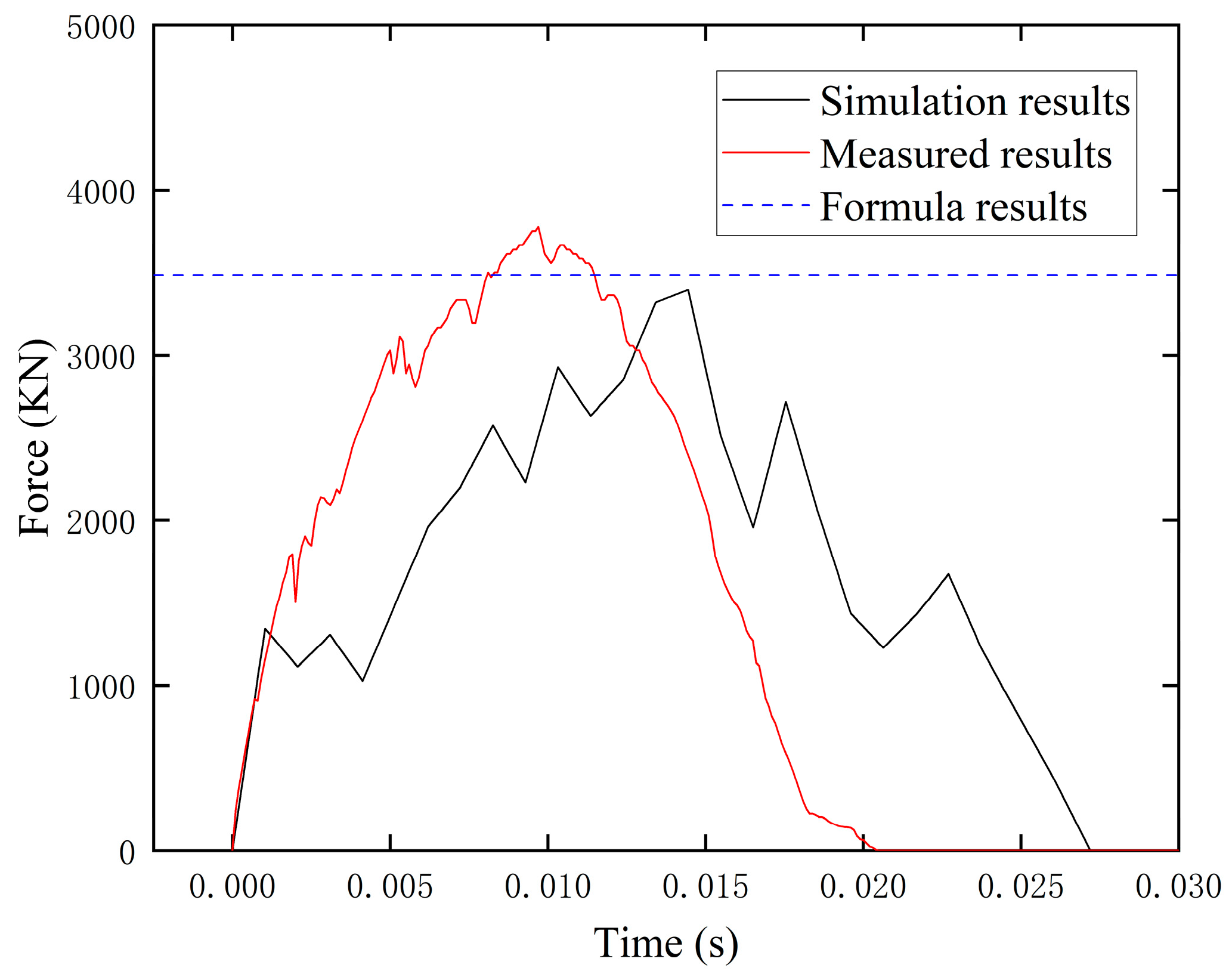
2.4. Validation of DEM

As shown in Figure 3, the maximum force obtained from the numerical simulation of the DEM of the impact particles of the flow ice and the bridge abutment is 3756.98 KN, which is 9.8% different from the measured maximum flow ice load of the Heihe–Blagoveshchensk Amur River Bridge in 2021 3388.8 KN, and 7.7% different from the ice pressure calculation method of 3485.93 KN stipulated in the Chinese General Specification for Design of Highway Bridges and Culverts (JTG D60-2015). The results show that the discrete element simulation value is more consistent with the measured value, which verifies the rationality of the DEM. The shorter duration of the single impact response of the simulation results compared to the measured values may be due to the fact that the actual ice is not uniformly distributed and material continuity is difficult to ensure, while the simulation method adopts the assumption of a homogeneous ice body, which accelerates the fracture response. In addition, the continuous impact of ice rows in the field produces a dynamic superposition effect, which enlarges the variability of the time–course characteristics. The above results show that the discrete element method can effectively simulate the transient impact process of ice loading.

2.5. Parameter Range Selection

The measured river ice velocity at the site of the Heihe–Blagoveshchensk Amur River Bridge in 2021 was between 0.386 m/s and 2.89 m/s, with a maximum of no more than 3 m/s. Therefore, a river ice velocity of 0.5–3.0 m/s was selected for numerical simulation in this paper. According to the literature [25], the maximum ice thickness of the Songhua River basin in Northeast China fluctuates in the range of 0.12–1.4 m, and the average ice thickness is between 0.5 and 0.75 m. Referring to this range, this paper sets the parameter range of river ice thickness between 0.2 and 1.5 m.

Existing literature on the sampling and study of river ice porosity is less abundant; with reference to the past scholars’ research on sea ice porosity [26], this paper selects the porosity interval of 5–30% for numerical simulation analysis, which basically can cover the range of common ice porosities.

3. Results and Discussion

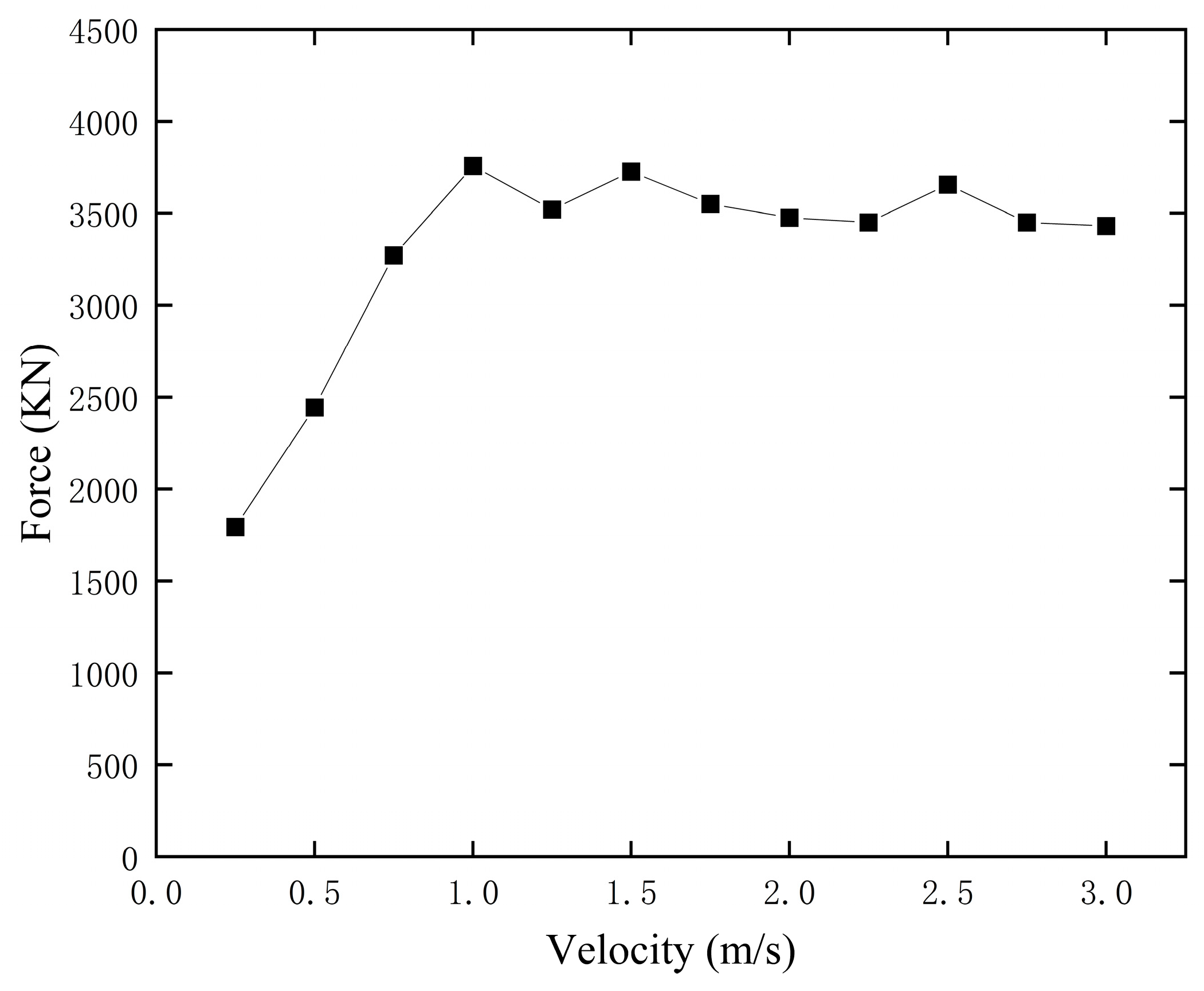
3.1. Influence of Ice Velocity on River Ice Impact Forces at Bridge Abutments

The river ice porosity is set to 0, the ice thickness is set to 0.5 m, and the ice velocities of 0.25 m/s, 0.5 m/s, 0.75 m/s, 1 m/s, 1.25 m/s, 1.5 m/s, 1.75 m/s, 2 m/s, 2.25 m/s, 2.5 m/s, 2.75 m/s, and 3 m/s are used for the discrete elemental simulation of the impact between the river ice and the bridge abutment. The time course of the ice force is illustrated in Figure 4, and the ice row damage at the simulation time of 1 s is shown in Figure 5.

River ice is the most common source of impact on bridge abutments; river ice in the river under the action of high-speed water flow impacts bridge abutments, provoking a bridge-structure response; the transient effect of the impact is intense, and has the most significant effect on the bridge abutment.

Ice rows have an impact on bridge abutments and other structures; when the speed is low, the driving force of the ice row on the impact to the bridge abutment is insufficient, and the ice row in the full width of the structure may be completely wedged into the scope of a full stop, shear or immediately rebound back. With the increase in ice speed, the ice row is partially embedded in the abutment but still cannot go further, then with the increase in kinetic energy of the ice row, the reaction force of the abutment to the ice row will gradually increase. At this time, the ice force manifests itself as a single amplitude of force, this stage of the ice row does not reach its destructive strength. When the ice speed continues to increase, reaching a certain critical speed point, the river ice’s driving force is sufficient, the ice row incurs partial or overall split damage. The ice row as a whole contains the destructive strength of the ice, and the river ice in contact with the front end region of the ice body incurs large-scale destruction, from the bearer to crushing and cracking after only a moment. At this time, the river ice impact force reaches its peak, and the subsequent impact force is manifested as multiple discrete peaks with lower ice force. As the ice velocity continues to increase, the river ice is not strong enough to support a larger impact force, and the magnitude of the maximum force is no longer determined solely by the ice velocity, but depends more on the ice strength. Eventually, the peak impact force stabilizes with the strength of the ice and does not continue to increase with velocity. Moreover, at high ice velocities, when the river ice reaches its maximum destructive strength, the size of the ice raft does not affect the impact force.

Figure 6 shows the maximum ice force applied to the bridge abutment at different ice velocities. As shown in the figure, the extreme value of the ice load increases significantly with the increase in velocity, and the ice load reaches the maximum value when the river ice velocity is 1 m/s. As the velocity continues to increase, the ice load’s extreme value eventually remains stable.

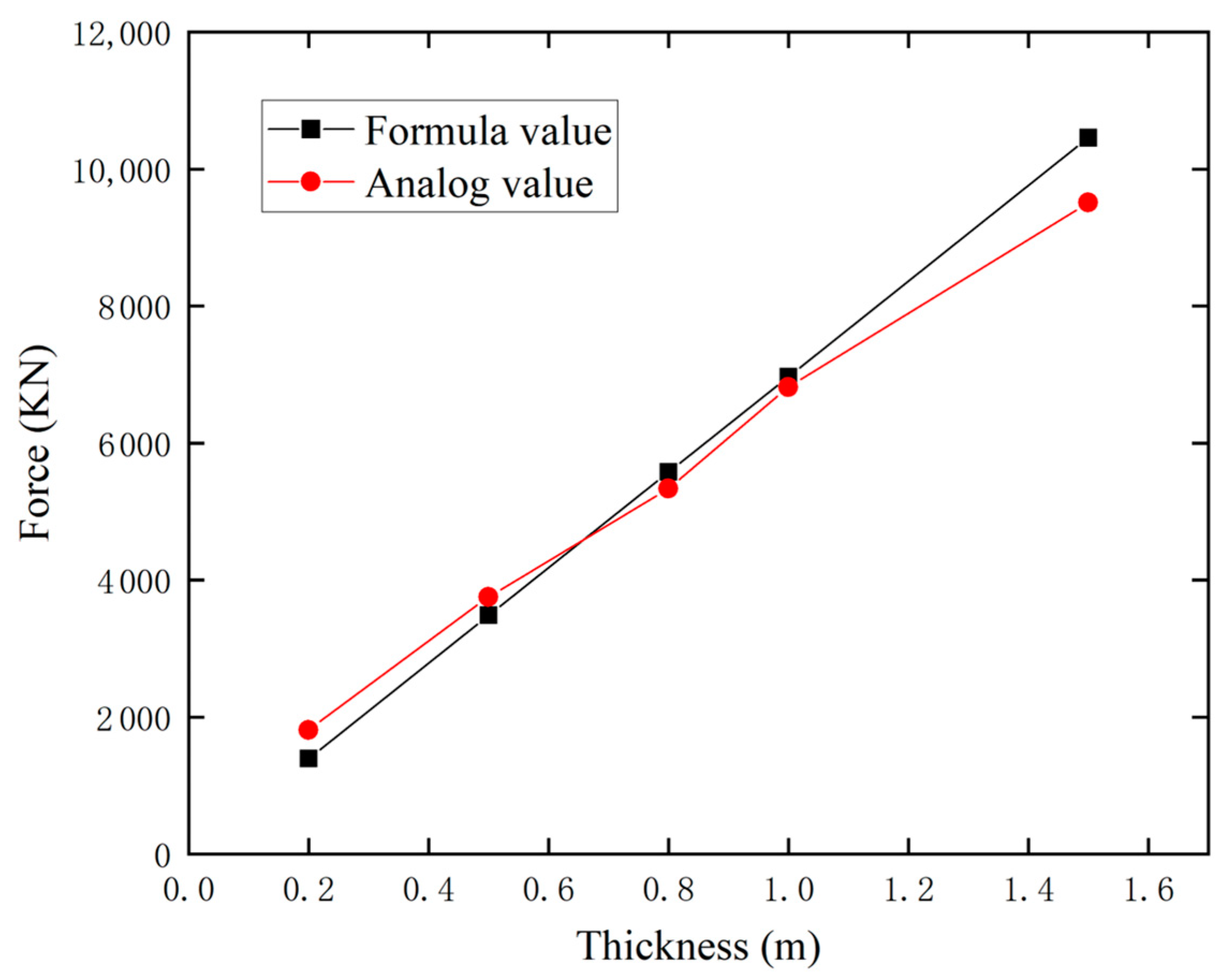
3.2. Influence of Ice Raft Thickness on River Ice Impact Forces at Bridge Abutments

The thickness of the ice row was set to 0.2 m, 0.5 m, 0.8 m, 1 m, and 1.5 m, and the discrete element simulation was carried out under the conditions of 0 porosity and 1 m/s velocity. The simulation results are shown in Figure 7. According to the simulation results, the peak impact force increases significantly with the increase in ice row thickness.

Figure 8 shows the comparison of the maximum impact force calculated from the simulation and the formula of the Chinese General Specification for Highway Bridge Culvert Design for different thicknesses of ice rows, and it can be found that the maximum impact force is basically proportional to the ice thickness in the two results.

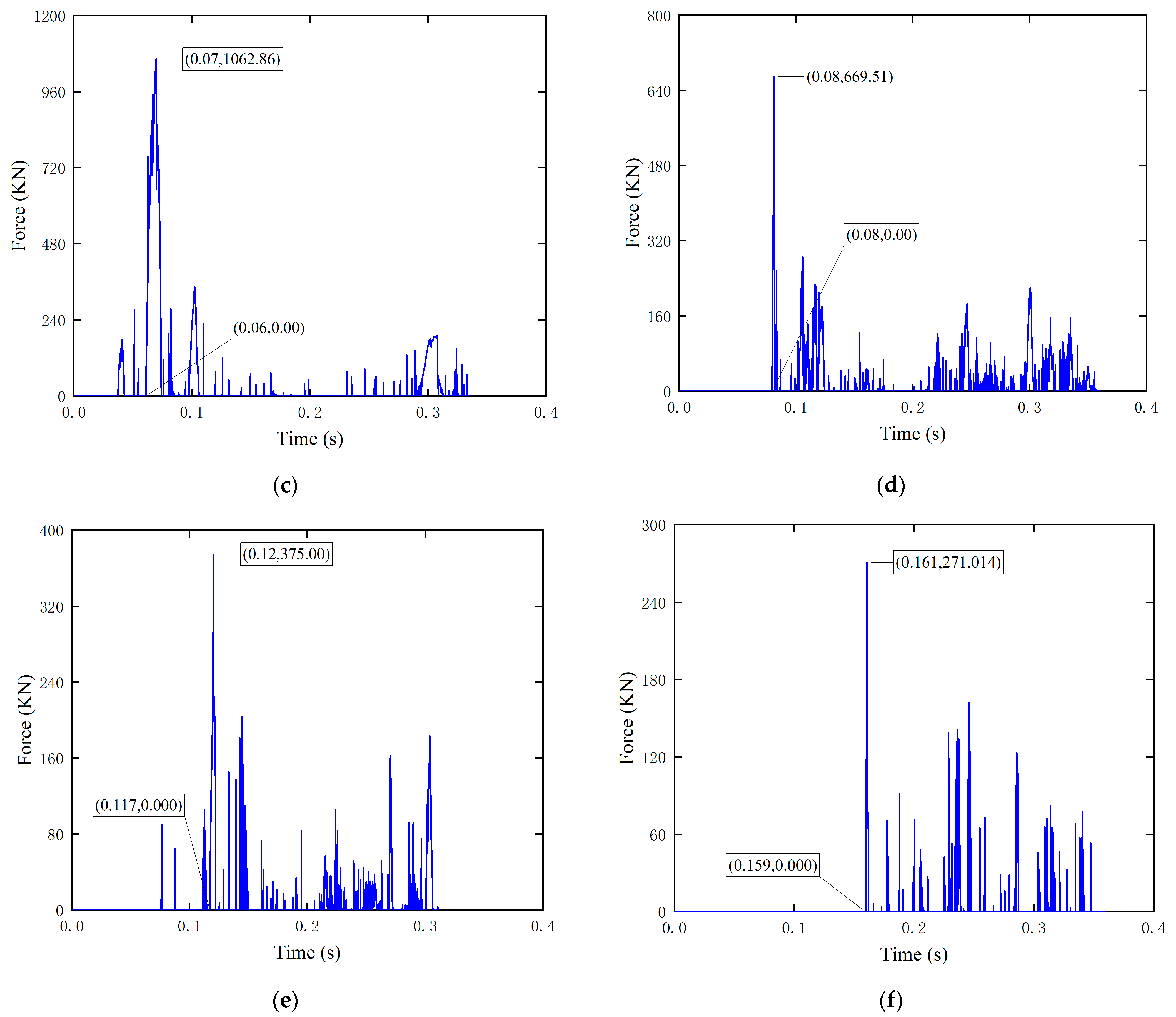
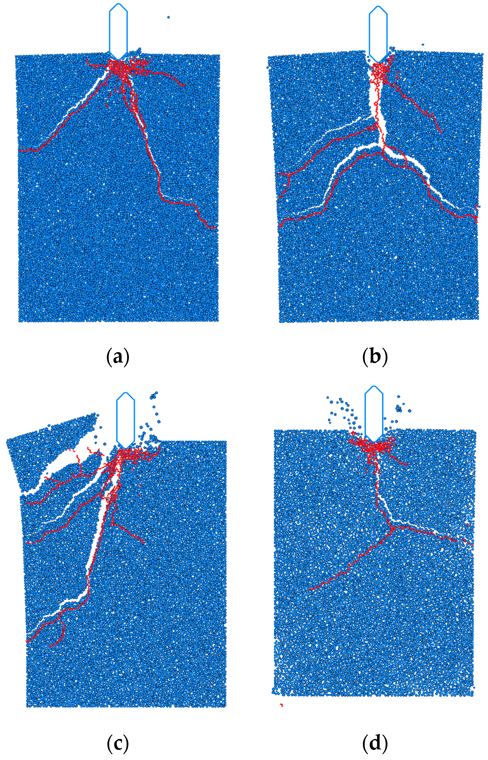
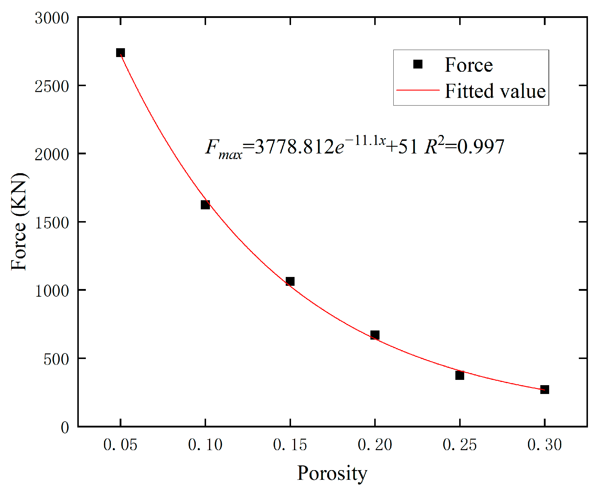
3.3. Influence of Porosity on River Ice Impact Forces at Bridge Abutments

The initial velocity of the river ice is established at 1 m/s, the thickness of the ice row is taken as 0.5 m, and the river ice porosities of 5%, 10%, 15%, 20%, 25%, and 30% are chosen to simulate the effect of the river ice porosity on the maximum impact force when the impact damage occurs. The simulated ice load time course is illustrated in Figure 9.

Table 2. Extreme values of ice load.

Porosity	Ice Load Extreme/KN
0.05	2739.8
0.1	1625.19
0.15	1062.8
0.2	669.1
0.25	375
0.3	271

, showing the role of ice load, clearly shows that as porosity increases, ice force at the abutment exhibits a consistent decrease. This phenomenon indicates that river ice porosity has a significant effect on the river ice impact force on the bridge abutment. When the porosity of the ice row increases, its internal structure becomes looser, and the strength of the river ice decreases, leading to a reduction in the ice row’s force on the bridge abutment in the process of breaking the ice.

In addition, as the porosity increases, the peak of the contact force is gradually lagged, and the time point at which the interaction between the bridge abutment and the ice raft begins to occur is delayed.

Finally, with the further increase in porosity, when the ice load reaches the extreme value and lags back, the subsequent time course begins to show the changing characteristics of random loading and unloading, which may be due to the complexity and instability of the internal structure of the ice row. In the ice row with higher porosity, the distribution and size of ice pores are more uneven, and the unbroken river ice extrudes forward to the abutment after the impact force reaches the peak, and encounters different sizes and shapes of pores during the penetration process, presenting the ice force time course with strong randomness and a lower peak value.

According to the ice row damage phenomenon under different porosities in Figure 10, it can be found that the damage pattern of the ice row changes with the increase in porosity. The damage is gradually concentrated near the face in contact with the ice-breaking column, and at high porosity, the abutment mainly has a destructive effect on the ice rows in the contact region, while it has less effect on the ice rows away from the contact region.

3.4. Construction of a Dynamic Load Model for River Ice Impacted Bridge Piers

From the characteristics of the impact force–time curve obtained from the simulation, it is evident that when the river ice impact damage occurs, the impact force of the river ice increases rapidly in a short period of time, and the impact force starts to decrease after reaching the peak value, so the impact process can be simplified into a triangular impact load, and the impact load graph can be determined by the four parameters of the peak value of the impact force, the loading time, the unloading time, and the start time of the river ice splitting. After the river ice reaches the maximum strength damage under high porosity, the time course of the ice force shows the lower discrete peak of the ice force, and the present model only considers the situation at the instant of river ice damage. The model is expressed as Equation (13).

$$F=\left\{\begin{array}{ll}{\displaystyle \frac{\begin{array}{l}{F}_{\max }\end{array}}{t_1}}\times (t-t_0)& (t_0<t\le t_1)\\ {\displaystyle \frac{F_{\max }}{t_2}}\times (t_1-t+t_0)+F_{\max }& (t_1\le t\le t_2)\end{array}\right.$$

(13)

3.4.1. Peak Impact Force

After the ice discharge flow velocity reaches the critical value, the size of Fmax is independent of the velocity and no longer increases. In this model, only the most unfavorable situation of river ice impact damage under high flow velocity is considered, and the maximum force when the river ice velocity is 1 m/s is taken as the peak impact force in the ice loading model, and the relationship between the river ice porosity and the extreme value of the impact force is obtained by fitting, as shown in Figure 11.

The simulation results clearly indicate that the ice force on the pier is negatively correlated with the porosity of the river ice, and with the increase in the porosity, the ice load reduction gradually decreases, which is in line with the strength of the river ice affected by the porosity. This nonlinear trend is consistent with the fact that the uniaxial compressive strength of ice is affected by porosity and that the change in ice strength with increasing porosity is the main reason for the impact force.

According to the statistical study of a large amount of data from sea ice compressive strength tests by previous scholars and summarizing the results of previous researchers [27], the relationship between compressive strength and porosity under the same strain rate mainly has the following expression:

$${\sigma }_c=A(1-\sqrt{p/B})$$

(14)

$${\sigma }_c=A(1-\sqrt{p})$$

(15)

$${\sigma }_c=A{(1-p)}^B$$

(16)

where ${\sigma }_c$ is the standardized value of the compressive strength of ice, and $A$ and $B$ are coefficients related to the strain rate. From the above expression, the compressive strength of the ice material is negatively correlated with the porosity or the square root of the porosity, which is corroborated by the DEM results of this study.

The porosity coefficient is introduced as a correction coefficient into the ice pressure calculation method stipulated in the Chinese General Specification for Highway Bridge and Culvert Design (JTG D60-2015), so the expression of the porosity-corrected one is as follows:

$$F_{\max }=m{C}_{t}bt{R}_{ik}{p}_0$$

(17)

where $F_{\max }$—standard value of calculated ice pressure (KN);

$m$—shape coefficient of ice-facing surface of bridge piers and pilings;

$C_t$—ice temperature coefficient;

$b$—projected width of bridge pier and pile facing ice surface (m);

$t$—river ice thickness (m);

$R_{ik}$—ice compressive strength standard value (KN/m)

$p_0$ versus river ice porosity $p$ is given as follows:

$$p_0=1.08e^{-7.4p}-0.064$$

(18)

3.4.2. Time Parameter

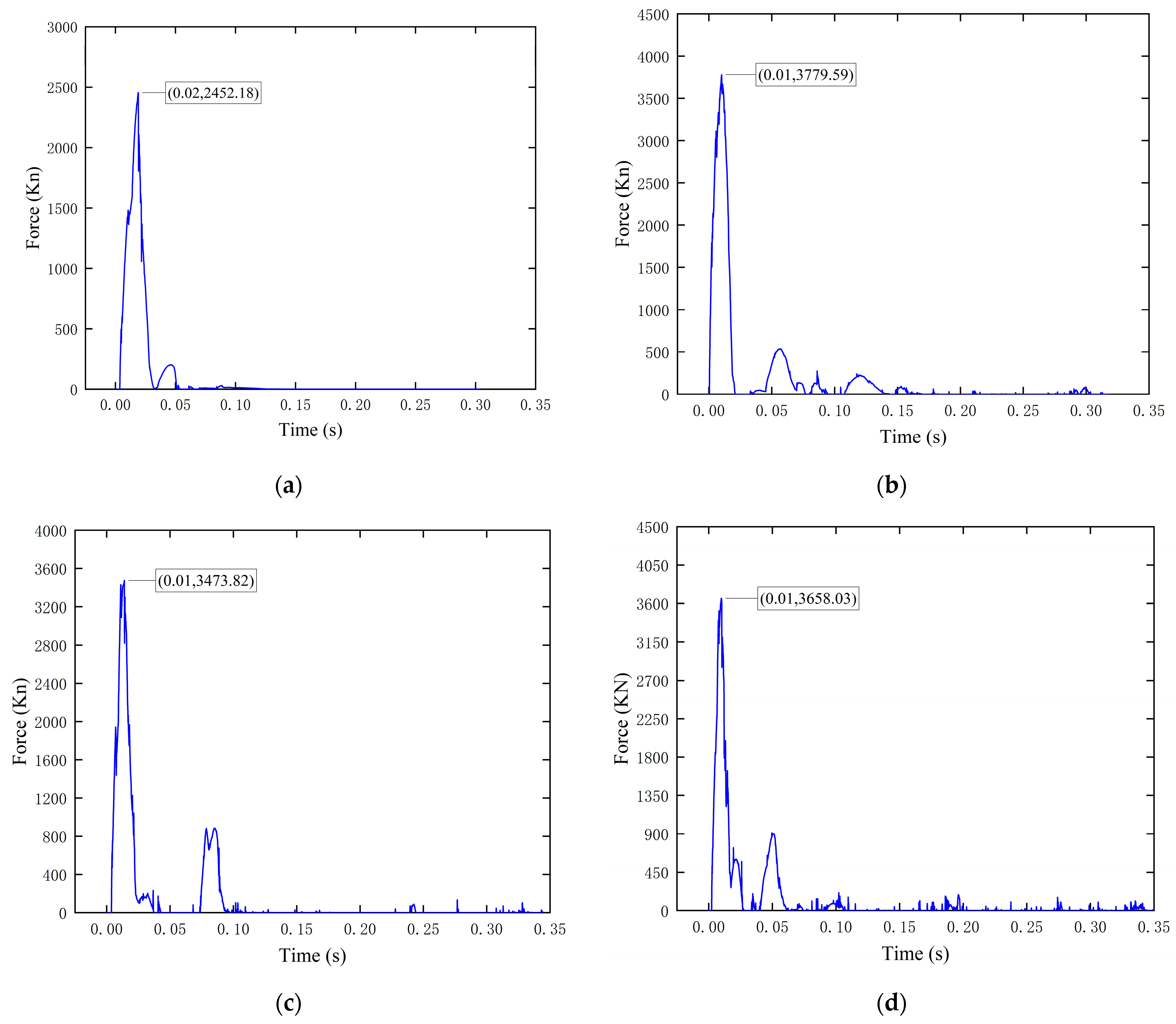
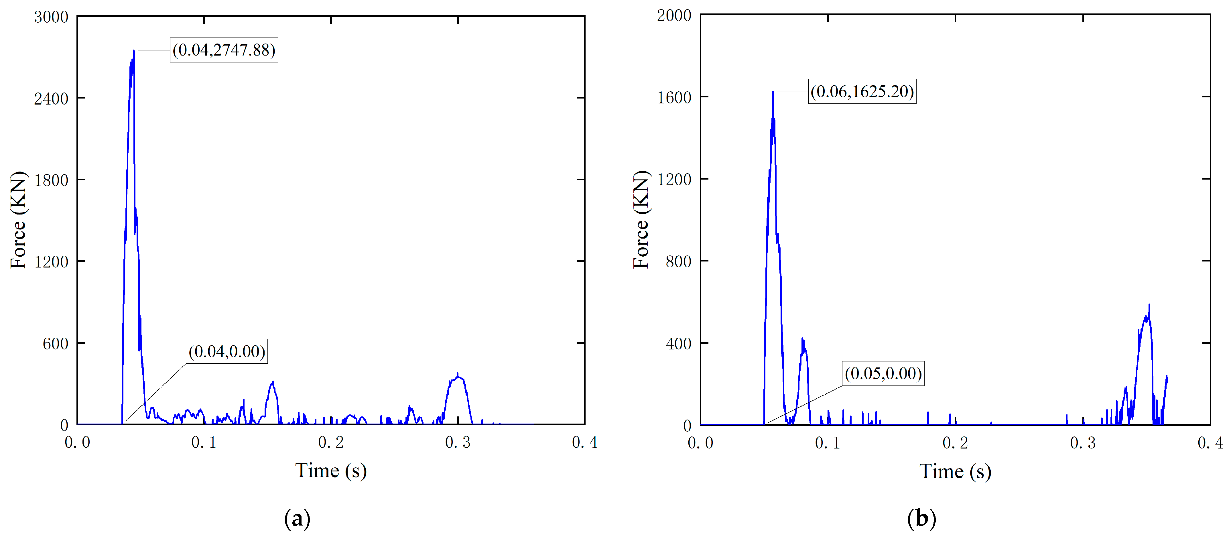
The time parameter of river ice impact is closely related to the damage form of the river ice, and there is a certain degree of randomness. However, by selecting the simulation results under different ice speeds, ice thicknesses, and porosities for comparative analysis, it is found that there is still a certain law for reference.

• Time of onset of river ice impact.
  As shown in Figure 12,with the increase in porosity, the degree of ice row loosening increases accordingly, and the piers need a longer time to reach the maximum destructive force when penetrating the river ice. According to the simulation results, with the increase in porosity, the onset time of river ice splitting increases, and the peak of contact force is gradually lagged. The relationship between river ice porosity and the onset time of impact is obtained by fitting, as shown in Figure 10. Changes in river ice velocity and ice thickness have a small effect on the onset time, so the onset time $t_0$ is expressed as a function of porosity $p$.

  $$t_0=0.01307e^{7.957p}+0.11$$

  (19)

2.

Load time and unload time.

As presented in

Table 3. Time parameters.

Porosity	Velocity (m/s)	Ice Thickness (m)	Onset Time (s)	Load Time (s)	Unload Time (s)
0	1	0.5	0.0004	0.0109	0.0168
		1	0.0009	0.0098	0.0188
		1.5	0.0006	0.0117	0.0155
0.05	1	0.5	0.04	0.0104	0.0151
	2		0.036	0.0065	0.0113
	3		0.032	0.005	0.0085
0.1	1	0.5	0.050	0.0084	0.0116
	2		0.044	0.0048	0.0089
	3		0.048	0.003	0.0063
0.15	1	0.5	0.065	0.0065	0.0079
	2		0.062	0.0046	0.0055
	3		0.060	0.0021	0.0039
0.2	1	0.5	0.085	0.0048	0.0041
	2		0.080	0.0029	0.0026
	3		0.083	0.0015	0.0017
0.25	1	0.5	0.117	0.004	0.0028
	2		0.111	0.0013	0.0013
	3		0.121	0.0006	0.0004
0.3	1	0.5	0.156	0.0034	0.0026
	2		0.159	0.0009	0.0013
	3		0.153	0.0004	0.0002

, with the increase in river ice porosity and river ice velocity, the time for the impact force to reach the peak and the time for the impact force to fall back from the peak both become shorter, and the loading time of the river ice impact is obviously faster than the unloading time, while the thickness of the ice raft has little effect on the loading time and unloading time of the river ice. The increase in river ice porosity reduces the strength of the river ice, the ice raft reaches its strength limit faster, the increase in velocity makes the stress on the ice raft accumulate more rapidly, generating more kinetic energy, and the loading time and unloading time of ice raft failure are shortened accordingly. According to the simulation results, the relationship between load time $t_1$, unload time $t_2$ and $vp(p\ne 0)$ is plotted and fitted, as shown in Figure 13. The load time $t_1$ and unload time $t_2$ of the river ice are expressed as a function of $vp$.

$$t_1=0.01e^{-4.76vp}+0.000504$$

(20)

$$t_2=0.02e^{-5.88vp}+0.000924$$

(21)

3.4.3. Load Model Validation

The dynamic load model of the river ice impacting on the bridge pier can be obtained by substituting the above parameter analysis results (17)–(21) into Equation (13). By comparing the discrete element simulation results of river ice with a porosity of 0.08, ice thickness of 0.5 m, ice speed of 2.5 m/s with the results of the load model, it can be found that the ice force time course calculated according to the two methods is relatively close to that shown in Figure 14. The comparison results of each parameter are shown in

Table 4. Comparison between simulation results and load modeling results.

Parameters	Simulation Results	Load Modeling Results	Inaccuracies
peak impact force/KN	1780	1936	−8.7%
Onset time/s	0.033	0.041	−5.8%
Load time/s	0.0054	0.005	8.7%
Unload time/s	0.006	0.0065	−7.5%

, in which the comparisons between the simulation results and the load model calculation results in each key parameter are listed in detail, and all of them show good consistency. It is evident that the river ice dynamic load model established in this paper more accurately simulates the process of the impact of the flow of ice on the bridge abutment of the Heilongjiang Bridge. In practical application, the method of this paper can be referred to, according to the specific bridge project, the ice load model used for further correction and improvement.

3.5. Engineering Applications

The traditional ice-resistant design of bridges usually adopts the static ice-loading method, whose crude assumptions ignore the influence of factors such as porosity, leading to a bipolar dilemma: over-conservative design triggers material redundancy or underestimation of the extreme ice conditions buries the hidden danger of structural safety. The dynamic ice-load function model constructed in this paper establishes a quantitative correlation between the physical properties of the ice sheet and the dynamic load by introducing the porosity correction coefficient, which provides a theoretical basis for design optimization. The risk-grading strategy based on this model can differentiate the design of bridges: additional floating steel-covered composite collision avoidance facilities are installed in the high-risk river section (low porosity, fast ice speed, thick ice), and structural simplification is carried out in the low-risk river section (high porosity, slow ice speed, thin ice) to realize lightweight construction and save the construction cost. In addition, by monitoring changes in porosity, the maintenance cycle of bridges can be dynamically adjusted, realizing the shift from empirical maintenance to data-driven predictive maintenance.

4. Conclusions

In this paper, a discrete element method was adopted to analyze the impact process and impact force of ablated river ice on bridge abutments by numerical simulation, the damage characteristics and impact force–time curve of ice rows under different ice speed and porosity conditions were obtained, and the relationship between the river ice porosity and the maximum impact force of the bridge abutment was fitted. The primary takeaways are as follows:

(1)

The simulation results indicate that increased ice speed significantly raises river ice impact force. When the speed of the ice reaches a certain critical threshold, the maximum impact force no longer increases with further increases in velocity. Instead, this peak impact force becomes more influenced by the strength of the ice. This finding is crucial for understanding how river ice interacts with bridges under extreme conditions.

(2)

The effect of river ice porosity on the impact force is also significant. As the porosity increases, the ice load decreases overall, while a lag occurs in the appearance of the peak contact force. In addition, the random loading and unloading characteristics of the ice load are enhanced, indicating that the change in porosity increases the uncertainty of the impact process, which puts forward higher requirements for the ice-resistant design of bridges in cold regions.

(3)

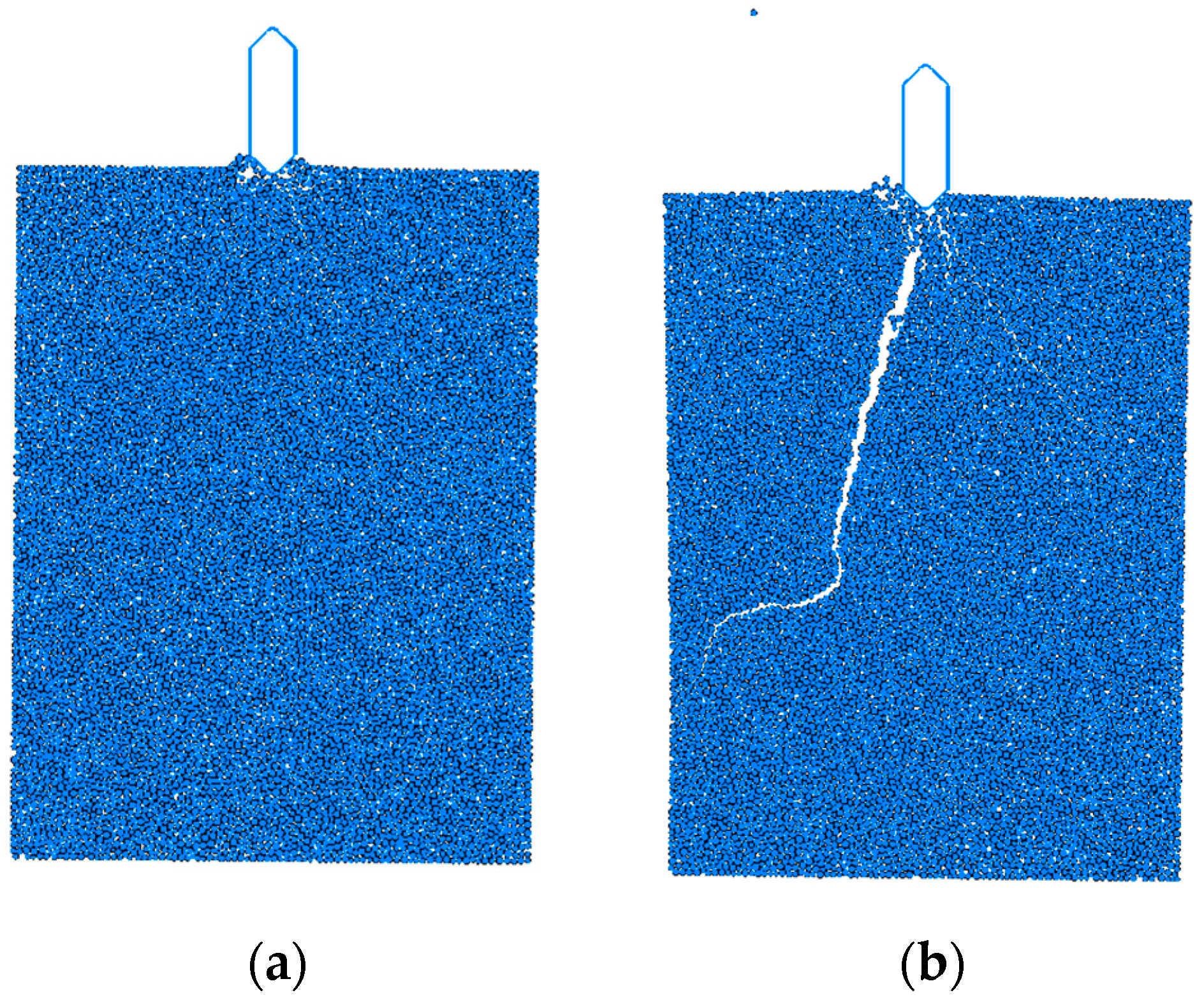
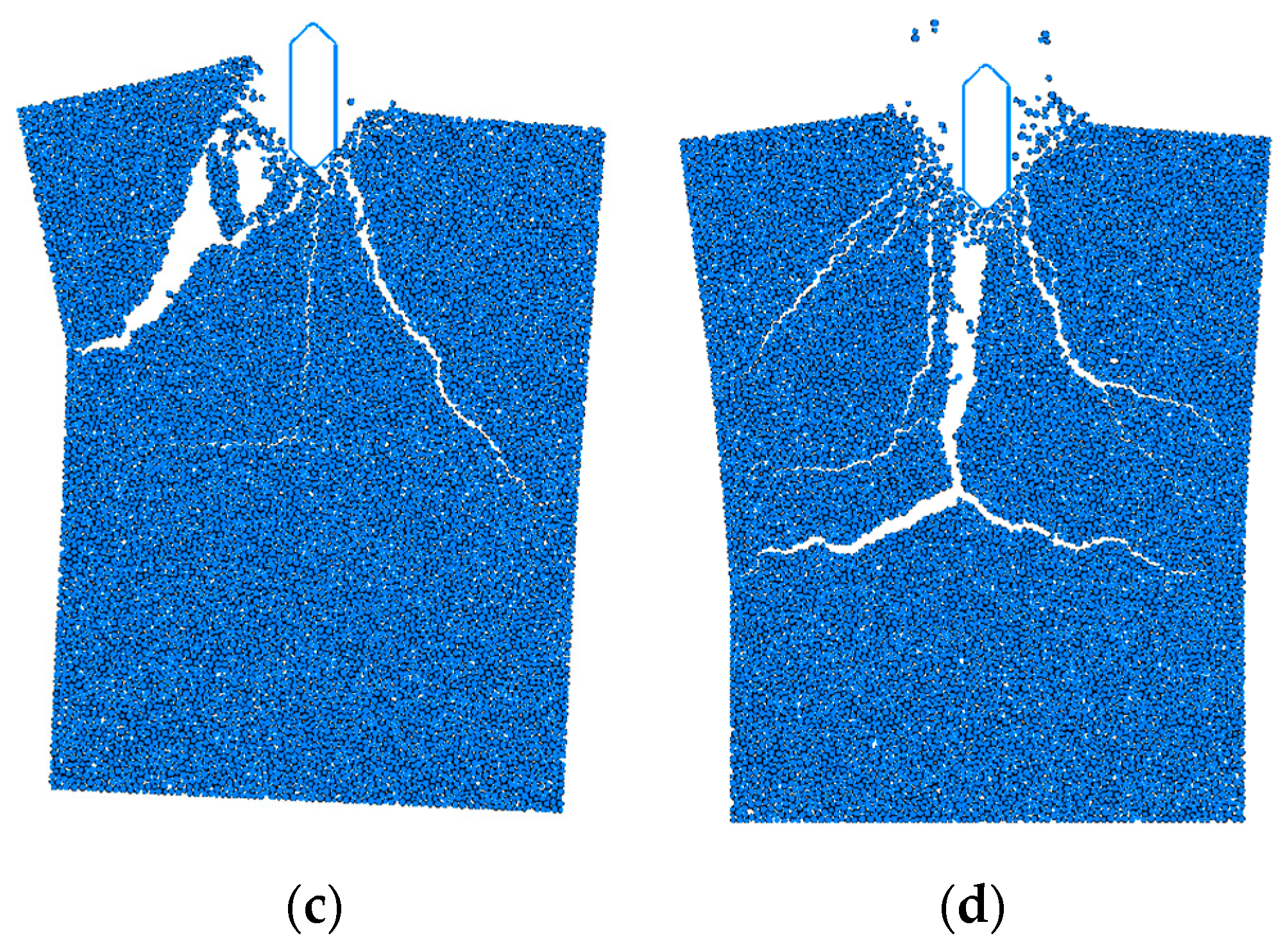
Regarding the damage pattern of ice rafts, it is found that with the increase in porosity, the damage is gradually concentrated near the area in direct contact with the bridge abutments. Therefore, emphasis should be placed on strengthening the protective capacity of the abutment-susceptible area to effectively resist the threat of ice collision.

(4)

According to the fitting results of the relationship between the river ice porosity and the maximum impact force, as well as each time parameter, the maximum impact force of the river ice gradually decreases with the increase in river ice porosity, and the fitting results show an obvious nonlinear relationship; the start time of the impact load increases with the increase in the porosity, and the loading time and unloading time decreases with the increase in the porosity and the ice speed. When analyzing and predicting the ice load on the structure, the effect of river ice porosity and the characteristics of the ice load model need to be fully considered.

(5)

This study focuses on revealing the effect of porosity on ice impact force but is limited by the model simplification: it has not yet covered the actual ice morphology diversity and impact location effect. The subsequent study will combine the discrete element modeling of U-shaped ice and irregular ice rows with the sensitivity analysis of the impact location, coupling multiple parameters, and providing domain-wide theoretical support for the ice-resistant design of bridges in cold regions.

References

1. Beltaos, S. River ice jams: Theory, case studies and applications. J. Hydraul. Eng. 1983, 109, 1338–1359. [Google Scholar] [CrossRef]
2. Matlock, H.; Dawkins, W.P.; Panak, J.J. Analytical Model for Ice-Structure Interaction. J. Eng. Mech. Div. 1971, 97, 1083–1092. [Google Scholar] [CrossRef]
3. Wong, C.K.; Brown, T.G. A Three-Dimensional Model for Ice Rubble Pile-Ice Sheet-Conical Structure Interaction at the Piers of Confederation Bridge, Canada. J. Offshore Mech. Arct. Eng. 2018, 140, 051501. [Google Scholar] [CrossRef]
4. Hendrikse, H.; Metrikine, A. Interpretation and prediction of ice induced vibrations based on contact area variation. Int. J. Solids Struct. 2015, 75, 336–348. [Google Scholar] [CrossRef]
5. Withalm, M.; Hoffmann, N. Simulation of full-scale ice–structure-interaction by an extended Matlock-model. Cold Reg. Sci. Technol. 2010, 60, 130–136. [Google Scholar] [CrossRef]
6. Zhang, S.F.; Yu, T.L. The Factors Sensitivity Analysis of Drift Ice Impact Force on the Pier. Adv. Mater. Res. 2014, 852, 472–475. [Google Scholar] [CrossRef]
7. Zhang, L.Z.; Xiong, W. Numerical Simulations of the Drifting Ice Sheets Collision with the Bridge Pier. Appl. Mech. Mater. 2013, 368, 1383–1386. [Google Scholar] [CrossRef]
8. Tuhkuri, J.; Polojärvi, A. A review of discrete element simulation of ice–structure interaction. Philos. Trans. R. Soc. A Math. Phys. Eng. Sci. 2018, 376, 20170335. [Google Scholar] [CrossRef] [PubMed]
9. Kärnä, T.; Turunen, R. Dynamic response of narrow structures to ice crushing. Cold Reg. Sci. Technol. 1989, 17, 173–187. [Google Scholar] [CrossRef]
10. Timco, G.W.; Nwogu, O.G.; Christense, F.T. Compliant model tests with the Great Belt West Bridge piers in ice Part II: Analyses of results. Cold Reg. Sci. Technol. 1995, 23, 165–182. [Google Scholar] [CrossRef]
11. Iliescu, D.; Baker, I. The structure and mechanical properties of river and lake ice. Cold Reg. Sci. Technol. 2007, 48, 202–217. [Google Scholar] [CrossRef]
12. Lu, Q.; Duan, Z.; Ou, J.; Wang, Z. Calculational method of river ice loads on piers (II): The formula for ice pressure. J. Nat. Disasters 2002, 11, 112–118. [Google Scholar] [CrossRef]
13. Jones, S.J. High Strain-Rate Compression Tests on Ice. J. Phys. Chem. B 1997, 101, 6099–6101. [Google Scholar] [CrossRef]
14. Moslet, P. Field testing of uniaxial compression strength of columnar sea ice. Cold Reg. Sci. Technol. 2007, 48, 1–14. [Google Scholar] [CrossRef]
15. Cole, D.M. The microstructure of ice and its influence on mechanical properties. Eng. Fract. Mech. 2001, 68, 1797–1822. [Google Scholar] [CrossRef]
16. Kharik, E.; Morse, B.; Roubtsova, V.; Fafard, M.; Côté, A.; Comfort, G. Numerical studies for a better understanding of static ice loads on dams. Can. J. Civ. Eng. 2018, 45, 18–29. [Google Scholar] [CrossRef]
17. Yue, Q.; Guo, F.; Kärnä, T. Dynamic ice forces of slender vertical structures due to ice crushing. Cold Reg. Sci. Technol. 2009, 56, 77–83. [Google Scholar] [CrossRef]
18. Sun, S.; Shen, H.H. Simulation of pancake ice load on a circular cylinder in a wave and current field. Cold Reg. Sci. Technol. 2012, 78, 31–39. [Google Scholar] [CrossRef]
19. Hopkins, M.A. Discrete element modeling with dilated particles. Eng. Comput. 2004, 21, 422–430. [Google Scholar] [CrossRef]
20. Hopkins, M.A.; Shen, H.H. Simulation of pancake-ice dynamics in a wave field. Ann. Glaciol. 2001, 33, 355–360. [Google Scholar] [CrossRef]
21. Shen, H.H.; Hibler, W.D.; Leppäranta, M. The role of floe collisions in sea ice rheology. J. Geophys. Res. Oceans 1987, 92, 7085–7096. [Google Scholar] [CrossRef]
22. Jiang, M.; Shen, Z.; Wang, J. A novel three-dimensional contact model for granulates incorporating rolling and twisting resistances. Comput. Geotech. 2015, 65, 147–163. [Google Scholar] [CrossRef]
23. Hillerborg, A.; Modéer, M.; Petersson, P.-E. Analysis of crack formation and crack growth in concrete by means of fracture mechanics and finite elements. Cem. Concr. Res. 1976, 6, 773–781. [Google Scholar] [CrossRef]
24. Liu, H. Study on Physical and Mechanical Properties of River Ice by Test and Discrete Element Numerical Simulation. Master’s Thesis, Harbin Institute of Technology, Harbin, China, 2022. [Google Scholar] [CrossRef]
25. Yang, Q.; Song, K.; Hao, X.; Wen, Z.; Tan, Y.; Li, W. Investigation of spatial and temporal variability of river ice phenology and thickness across Songhua River Basin, northeast China. Cryosphere 2020, 14, 3581–3593. [Google Scholar] [CrossRef]
26. Timco, G.W.; Weeks, W.F. A review of the engineering properties of sea ice. Cold Reg. Sci. Technol. 2010, 60, 107–129. [Google Scholar] [CrossRef]
27. Li, Z.; Zhang, L.; Lu, P.; Leppäranta, M.; Li, G. Experimental study on the effect of porosity on the uniaxial compressive strength of sea ice in Bohai Sea. Sci. China Technol. Sci. 2011, 54, 1331–1334. [Google Scholar] [CrossRef]
Figure 1. Parallel bonded contact model.
Applsci 15 01738 g001
Figure 2. Abutment cross-section of the Heihe–Blagoveshchensk Amur River Bridge.
Applsci 15 01738 g002
Figure 3. Comparison of different ice load impacts.
Applsci 15 01738 g003
Figure 4. Time course of ice force at different ice speeds: (a) 0.5 m/s; (b) 1 m/s; (c) 2 m/s; (d) 2.5 m/s.
Applsci 15 01738 g004
Figure 5. Ice raft destruction patterns at different ice velocities: (a) 0.5 m/s; (b) 1 m/s; (c) 2 m/s; (d) 2.5 m/s.
Applsci 15 01738 g005aApplsci 15 01738 g005b
Figure 6. Maximum ice force on bridge abutment at different ice speeds.
Applsci 15 01738 g006
Figure 7. Maximum ice force on bridge abutment under different ice thicknesses.
Applsci 15 01738 g007
Figure 8. Comparison of simulated and formula-calculated maximum impact force for different ice row thicknesses.
Applsci 15 01738 g008
Figure 9. Time course of ice loading with different porosities: (a) 5%; (b) 10%; (c) 15%; (d) 20%; (e) 25%; (f) 30%.
Applsci 15 01738 g009aApplsci 15 01738 g009b
Figure 10. Ice discharge damage pattern with different porosities: (a) 5%; (b) 10%; (c) 15%; (d) 20%; (e) 25%; (f) 30%.
Applsci 15 01738 g010aApplsci 15 01738 g010b
Figure 11. Relationship between river ice porosity and maximum ice force.
Applsci 15 01738 g011
Figure 12. Relationship between porosity and onset time.
Applsci 15 01738 g012
Figure 13. Load time, unload time vs. vp: (a) load time fitting results; (b) unload time fitting results.
Applsci 15 01738 g013
Figure 14. Comparison between simulation results and load modeling results.
Applsci 15 01738 g014