Cooperative Formation Control of a Multi-Agent Khepera IV Mobile Robots System Using Deep Reinforcement Learning

Abstract

The increasing complexity of autonomous vehicles has exposed the limitations of many existing control systems. Reinforcement learning (RL) is emerging as a promising solution to these challenges, enabling agents to learn and enhance their performance through interaction with the environment. Unlike traditional control algorithms, RL facilitates autonomous learning via a recursive process that can be fully simulated, thereby preventing potential damage to the actual robot. This paper presents the design and development of an RL-based algorithm for controlling the collaborative formation of a multi-agent Khepera IV mobile robot system as it navigates toward a target while avoiding obstacles in the environment by using onboard infrared sensors. This study evaluates the proposed RL approach against traditional control laws within a simulated environment using the CoppeliaSim simulator. The results show that the performance of the RL algorithm gives a sharper control law concerning traditional approaches without the requirement to adjust the control parameters manually.

1. Introduction

In recent years, AI has enabled machines to perform tasks typically requiring human intelligence including visual perception, speech recognition, decision-making, and language translation, transforming numerous fields [1,2,3]. Among AI’s many applications, machine learning (ML) stands out, enabling algorithms to learn from data and make predictions or decisions without explicit programming [4]. A further specialization within the field of machine learning is deep learning (DL), which utilizes neural networks with multiple layers to model intricate patterns in extensive datasets [5,6,7,8].

Deep learning algorithms, particularly those involving reinforcement learning, have shown great promise in enabling agents to develop sophisticated strategies through trial and error [9,10]. By leveraging neural networks, these agents can process vast amounts of sensory data, identify patterns, and make informed decisions. This is particularly beneficial in scenarios where agents must operate collaboratively to achieve a common goal [11].

The integration of DL with multi-agent systems has seen a marked increase in interest recently [12,13], particularly in the context of mobile robot formation control [14]. This innovative approach utilizes the power of DL to enable multiple autonomous agents to learn and adapt their behaviours by interacting with their environment and each other [15]. The primary objective is to achieve and maintain specific formations, crucial for applications ranging from unmanned aerial vehicle (UAV) swarms to autonomous vehicle platoons [16,17]. By addressing the complexities of coordination, communication, and dynamic environments, DL offers a promising solution to enhance the efficiency and robustness of multi-robot systems.

During the last few years, our research has focused on the position control of mobile robots [18], leveraging advanced deep reinforcement learning algorithms. Our previous work [19,20] details the design, development, and implementation of reinforcement learning algorithms for controlling the position of a wheeled mobile robot Khepera IV. These approaches facilitate the learning of optimal control policies through environmental interaction, resulting in significantly improved performance compared with traditional control methods [21,22,23,24]. Our experiments, conducted both in simulation and real-world environments, demonstrate the effectiveness of our algorithms in achieving precise position control, even in the presence of obstacles.

This work presents innovative models that enable autonomous agents to learn and adapt their behaviours using deep reinforcement learning (DRL). These models show the potential of this approach in applications such as UAV swarms and autonomous vehicle platoons. This research addresses the complexities of coordination and communication required to maintain precise formations. Using DRL, the models allow multiple agents to process large amounts of data in real-time. This enables them to make better decisions and adjust their positions dynamically. This capability ensures the agents can operate cohesively, maintaining their formation even in dynamic and unpredictable environments. The enhanced coordination and communication lead to increased efficiency and robustness of multi-robot systems, making them more reliable and effective in various scenarios. This work’s findings could significantly improve autonomous systems, from transportation and surveillance to other fields.

The main contributions of this work are as follows:

• Design and implementation: The design and implementation of a control law for the formation position control of a group of robots based on DRL. This control law helps robots maintain precise formations and adapt to their surroundings, improving on the results presented in [18], where classical controllers were used.
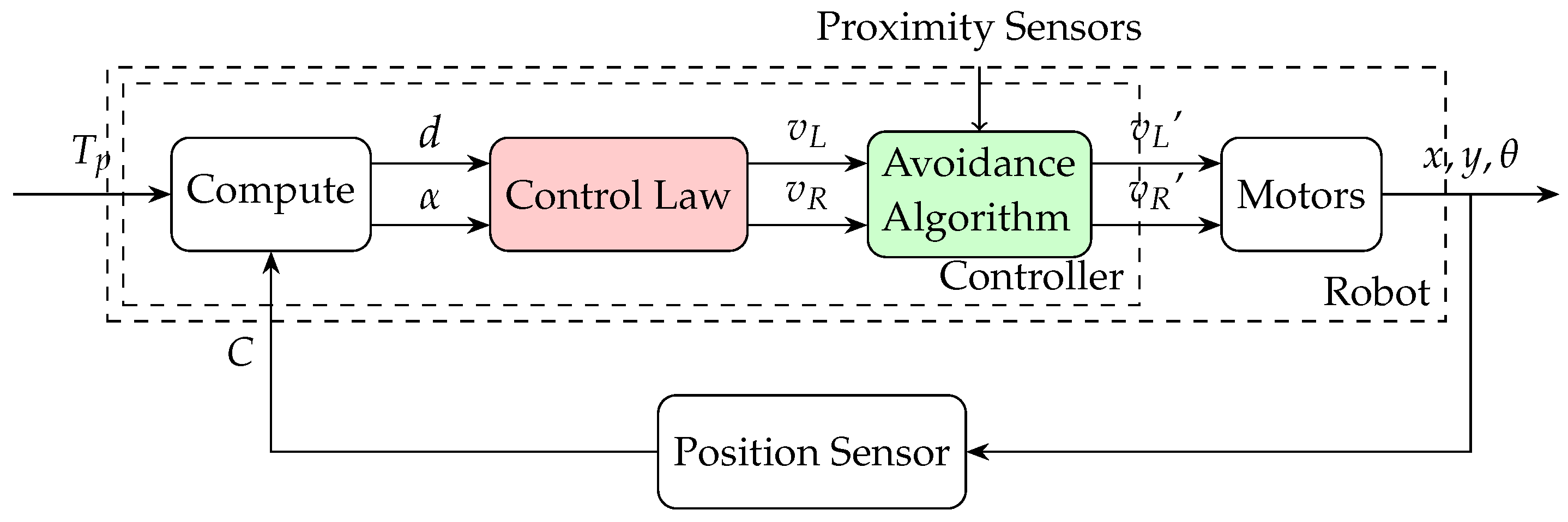
• Simulation environment: The implementation of the proposed algorithm in a simulation environment, including obstacle avoidance. This enables thorough testing and validation of the effectiveness of the algorithm in maintaining formation and avoiding obstacles. The obstacle avoidance logic presented in [19] was expanded to all robots in the formation.
• Comparison with traditional position control approaches: Comparison of the results of the new approach against existing control laws under similar conditions. This comparison highlights the advantages and improvements offered by the RL-based method. This work expands on [20] by experimenting with a more explicit reward function for faster target tracking.
• Performance evaluation: The evaluation of the performance of the proposed control law using their control surfaces. This provides a quantitative assessment of the algorithm’s efficiency, robustness, and adaptability. Similar metrics as used in [19] were selected for a more accurate comparison.

The remainder of this paper is organized as follows: Section 2 presents the environment where the experiments will take place, as well as some theoretical aspects of the position control problem, the formation control problem, the obstacles avoidance approach, and the multi-agent system. Section 3 describes the proposed approach: formation control with deep reinforcement learning. Section 4 shows and discusses some simulation and experimental results of this research. Finally, Section 5 presents the main conclusion and future works.

2. Background

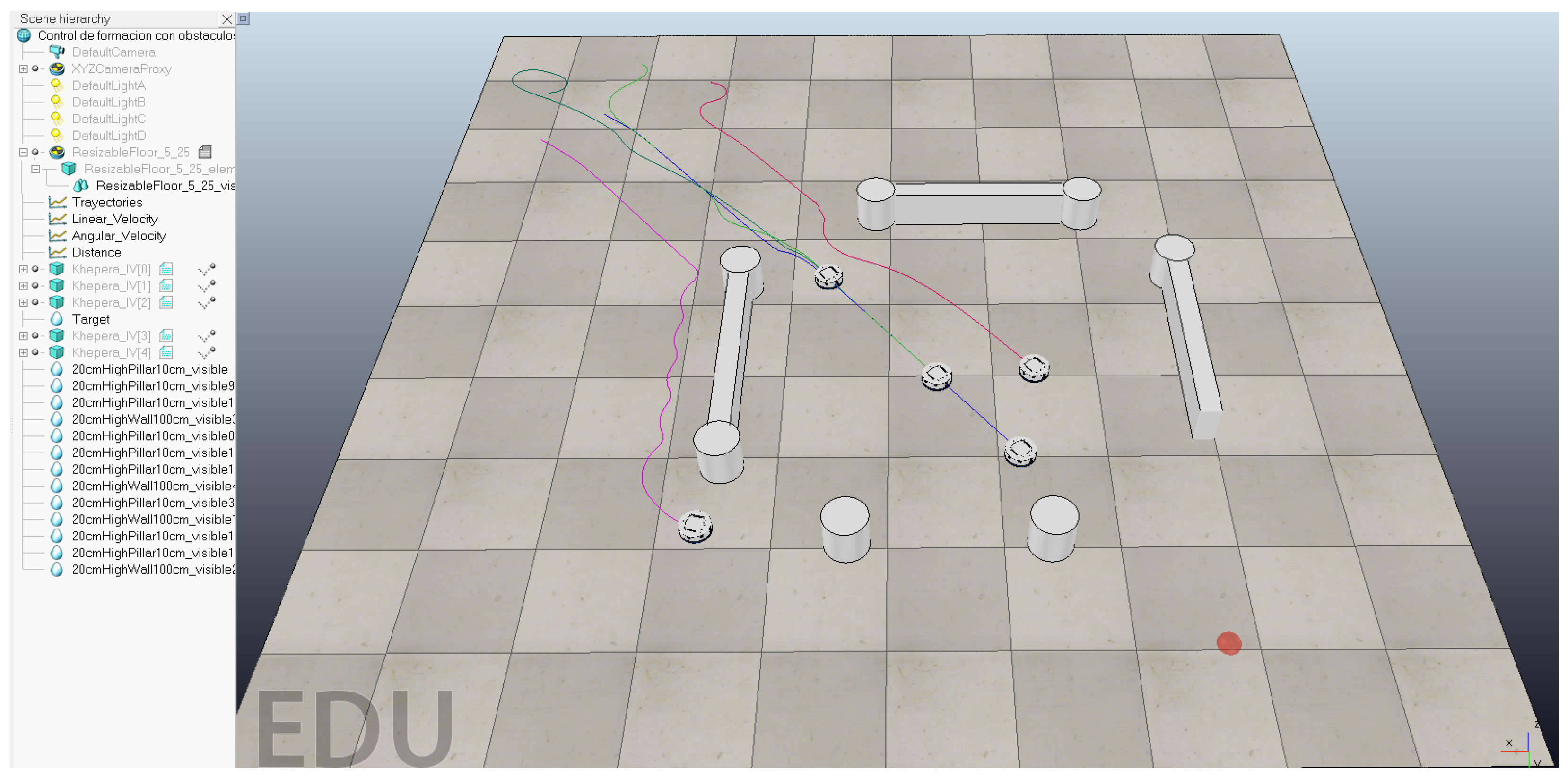
2.1. Simulation Environment—CoppeliaSim Simulator

CoppeliaSim simulator (formerly V-REP) [25] is a useful tool for the development of 3D simulations, based on high-fidelity physics-based models. As an integrated development environment (IDE), it allows for a distributed control architecture where each object/model can be individually controlled using embedded scripts, plug-ins, remote application program interface (API) clients, Robot Operating System (ROS) nodes, or custom solutions. On the other hand, control algorithms can be written in several programming languages, including Lua, C/C++, Python, MATLAB, Java, and others. The simulator offers numerous examples like robot models, sensors, and actuators to create and interact in a virtual world in real-time. Additionally, it allows for adding new objects with dynamic properties for designing and constructing new robots. In particular, a model for the Khepera IV robot has already been put together and developed for the CoppeliaSim simulator. In previous works [26] (see Figure 1), the authors developed a library to include the Khepera IV robot model in CoppeliaSim. In this work, the model of the Khepera IV is used to test the experiments in the CoppeliaSim environment.

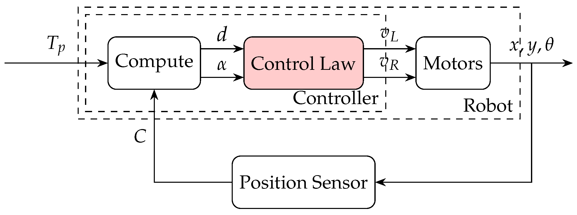
2.2. Robot Position Control

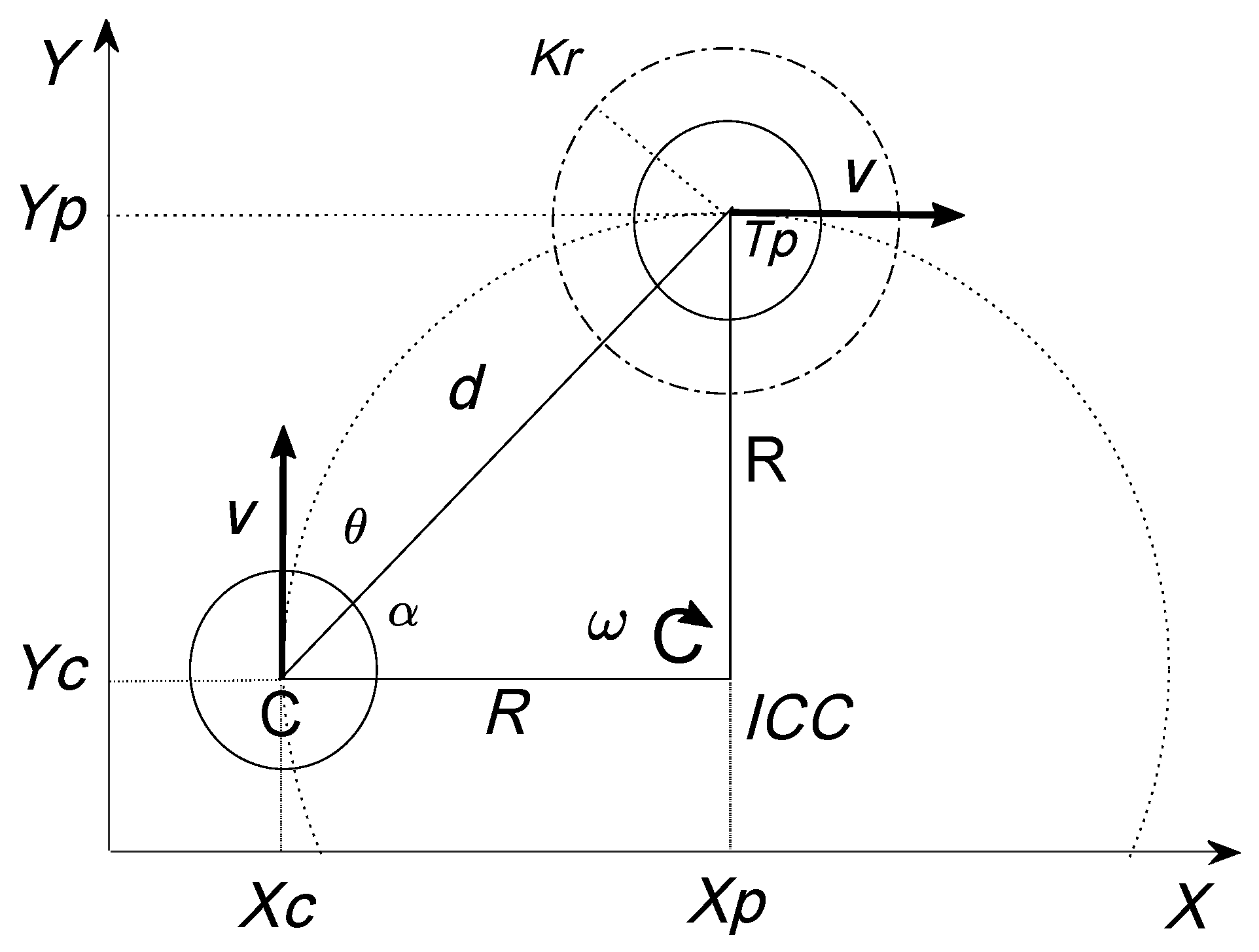
2.2.1. Kinematic Model for the Robot

A differential wheeled robot is a mobile vehicle that moves using two independently driven wheels located on either side of its body. The tangential velocities of these wheels denoted as ($v_L$) and ($v_R$), left and right, respectively, are perpendicular to the axis of the wheels. The wheels are assumed to roll without sliding, a restriction known as non-holonomic [27]. The robot changes direction by the differential rotation of the wheels, eliminating the need for an additional steering mechanism. The robot’s kinematic model in Cartesian coordinates is described as follows [23,28]:

$$\left\{\begin{array}{c}{\dot{x}}_c=vcos\left(\theta \right)\\ {\dot{y}}_c=vsin\left(\theta \right)\\ \dot{\theta }=\omega ,\end{array}\right.$$

(1)

where $(x_c,y_c)$ is the robot’s position, and $\theta$ is the heading direction angle, perpendicular to the turning radius (R). The linear and angular velocities of the robot are obtained from $V=(v_L+v_R)/2$, and $\omega =(v_L-v_R)/L$, respectively, with being L the distance between the wheels. The angular velocity is defined concerning the Instantaneous Center of Curvature (ICC). The robot has a maximum linear velocity $V_{max}$ and angular ${\omega }_{max}$, and a minimum turning radius $R_{min}$. It can only move forward or backward in the heading direction; this is known as non-holonomic constraints [24].

2.2.2. Position Control Problem

The experiment involves moving the robot from its current position (C) to a target point ($Tp$) by adjusting its angular and linear velocities. Traditionally, these velocities are generated by the controller and then transformed into speeds for the left and right motors. The proposed DRL directly outputs the wheels’ velocities. Figure 2 shows the variables involved in this experiment.

The kinematic behavior of these robots appears simple, but non-holonomic constraints pose a challenge in control law design. Previous works detail this issue, [24,29]. In typical motion, the differential robot follows a circular trajectory with radius R and center $ICC$. The position control algorithm aims to minimize orientation error ($e=\alpha -\theta$), where $\alpha$ is the angle to the target, and $\theta$ is robot orientation. Simultaneously, the robot decreases the distance to the target point ($d\to 0$).

Figure 3 illustrates the position control algorithm, with the inner square as the controller and the outer square as the robot. The Position Sensor is an IPS (Indoor Positioning System), providing the absolute position and orientation of the robot [18].

Equation (2) gives the distance d, and Equation (3) computes the angle to the target point $\alpha$, using the coordinates of $Tp(x_p,y_p)$ and $C(x_c,y_c)$. Both equations are part of the Compute block [24].

$$d=\sqrt{{\left(y_p-y_c\right)}^2+{\left(x_p-x_c\right)}^2}$$

(2)

$$\alpha ={tan}^{-1}\left({\displaystyle \frac{y_p-y_c}{x_p-x_c}}\right)$$

(3)

The algorithm calculates the wheel speeds required to reach the destination point based on distance and angle. This is performed using the block labeled Control Law (in light red color), which can be designed in different ways. One approach, known as Villela [21], generates control signals V and $\omega$ using the following equations:

$$\begin{array}{c}V\left(t\right)=\left\{\begin{array}{cc}{V}_{max}\hfill & if\hspace{1em}d>k_r\hfill \\ d{\displaystyle \frac{V_{max}}{k_r}}\hfill & if\hspace{1em}d\le k_r\hfill \end{array}\right.\hfill \end{array}$$

(4)

$$\omega ={\omega }_{max}sin\left(\alpha -\theta \right)$$

(5)

with $V_{max}$ and ${\omega }_{max}$ as defined before, and $K_r$, a docking area radius. This docking area allows a fast approach to the target when situated further away, but then slowing down nearby. From the robot’s velocities, the wheels’ (left and right) velocities are obtained by the relations $v_L=(2V+\omega L)/2$ and $v_R=(2V-\omega L)/2$.

2.3. Obstacles Avoidance (Braitenberg Algorithm)

The obstacles avoidance algorithm block (light green) is shown in Figure 4. It implements the Braitenberg algorithm for calculating new velocities ($v_L$’, $v_R$’) when obstacles are present nearby [30]. If no obstacles are detected, the output velocities remain the same as the input velocities for the block ($v_L^{\prime }=v_L$, $v_R^{\prime }=v_R$).

The Braitenberg algorithm uses sensor inputs (such as infrared or ultrasonic sensors) to control the motors of a robot. The basic idea is to connect the sensors to the motors in a way that the robot can react to its environment. Broadly speaking, when the left sensor detects an obstacle, it reduces the speed of the right motor, causing the robot to turn left.

Similarly, when the right sensor detects an obstacle, it reduces the speed of the left motor, causing the robot to turn right. This simple mechanism allows the robot to navigate around obstacles effectively. The adjustment between the sensors and the motors can be empirically calibrated by conducting a series of tests in different environments to observe the robot’s behavior. This helps in fine-tuning the sensor thresholds and motor responses to ensure smooth and effective obstacle avoidance [31].

2.4. Multi-Agent Systems

Multi-agent systems (MASs) consist of multiple interacting agents that work together to achieve a common goal. These systems are characterized by their ability to operate decentralized, where each agent makes decisions based on local information and interactions with other agents. This approach offers several advantages, including increased robustness, scalability, and flexibility [32].

In cooperative multi-agent systems, agents interact together to maximize a shared objective. This requires effective communication and coordination among agents to ensure that their actions are aligned toward the common goal. Examples of cooperative MASs include swarm robotics [33], where multiple robots collaborate to perform tasks such as search and rescue [34], environmental monitoring, and formation control.

To implement cooperation among agents, the interaction can be established in two different ways: (1) all agents have the same hierarchy/rank, and (2) there is a leader or master and the rest are followers. In the first approach, known as egalitarian cooperation, all agents collaborate equally, sharing information and decisions to achieve a common goal. This model promotes robustness and flexibility, as it does not rely on a single point of failure.

In the second approach, known as hierarchical cooperation, a leader or master agent coordinates the actions of the other agents, who act as followers. This model can be more efficient in terms of decision-making and coordination, especially in complex tasks that require centralized direction. Both approaches have their advantages and challenges, and the choice between them depends on the nature of the task and the environment in which the agents operate. To make a formation with the leader-follower approach, the following equations can be taken into account [35], where N is the number of followers:

$$v_m\left(t\right)=K_p{E}_{pm}\left(t\right)-K_f{E}_f\left(t\right)$$

(6)

$$d_s\left(t\right)=\sum _{i=1}^N{d}^{f_i}\left(t\right)$$

(7)

In the case of the followers, they use the position of the leader as a target point and a distance regarding their position in the formation concerning the leader. These equations help in designing the control strategy for the followers to maintain a specific formation relative to the leader. The velocity of the leader ($v_m\left(t\right)$) depends on two terms (Equation (6)): $K_p{E}_{pm}\left(t\right)$ which is its position error ($E_{pm}\left(t\right)$) and a control gain ($K_p$) that defines the importance of this error in the control. The second term ($-K_f{E}_f\left(t\right)$) represents the sum of the position error of each follower ($E_f$) in the formation (Equation (7)), multiplied by a control gain ($K_f$). By adjusting the control gains ($K_p$, $K_f$) and desired positions, the formation can be maintained dynamically as the leader moves.

Figure 5 shows a representation of non-cooperative multi-agent systems [36] from points A to C. The leader robot is represented in red and the followers in black. The dotted lines represent the distances between the leader and the follower robots.

The experiment starts at point A, where the position of the robots is not in formation, which is reached at point C. All the robots move from the initial position to point B (dashed lines), as can be seen, the leader does not wait for the followers and the formation is not maintained. Then, the leader arrives at point C and the followers take time to reach the final formation at point C. On the other hand, the example of cooperative multi-agent systems is shown from point C to E. The robots maintain the formation during the maneuver.

Deep Reinforcement Learning and Multi-Agent Systems

Multi-agent systems have a wide range of applications across various domains. In robotics, a MAS is used for tasks such as formation control, where multiple robots maintain a specific formation while navigating through an environment. This is particularly useful in scenarios involving unmanned aerial vehicles (UAVs) and autonomous vehicle platoons, where maintaining precise formations is crucial for efficiency and safety.

In addition to robotics, MASs are employed in fields such as distributed sensing, where multiple sensors work together to monitor and collect data from large areas. This approach enhances the coverage and accuracy of the sensing system, making it suitable for applications like environmental monitoring and surveillance.

Despite their advantages, multi-agent systems also face several challenges. One of the primary challenges is ensuring effective communication and coordination among agents, especially in dynamic and unpredictable environments. Developing robust algorithms that can handle these complexities is an ongoing area of research. Another challenge is the scalability of MASs, as the number of agents is incremented, the system’s complexity grows exponentially. Researchers are exploring techniques such as hierarchical organization and distributed control to address scalability issues [12].

Looking ahead, the integration of deep reinforcement learning (DRL) with multi-agent systems holds great promise. DRL enables agents to learn and adapt their behavior through interactions with their surroundings, making it a powerful tool for enhancing the capabilities of MASs. Future research will likely focus on developing more efficient and scalable DRL algorithms for multi-agent systems, paving the way for advanced applications in areas such as autonomous transportation, smart grids, and collaborative robotics [37].

3. Proposed Approach

Based on the leader/follower configuration, two different DRL controllers are designed. While the leader’s goal is to approach the target taking into consideration the location of the followers, the aim of these ones is to keep a fixed relative location concerning the leader for a given geometric formation. These relative reference positions are located on each side of the leader at some relative angle and distance. Both DRL controllers output the linear velocities of the left and right wheels, $v_L$ and $v_R$, according to Figure 3 or Figure 4.

The Deep Deterministic Policy Gradient (DDPG) is selected for the DRL controllers. This is an improvement derivation from the Q-learning and Deep Q-learning Controller (DQN) formulations for continuous-time states and actions based on the following recursive Bellman optimality equation [38]:

$$\begin{array}{c}Q\left(S\right[k],A[k\left]\right)=Q\left(S\right[k],A[k\left]\right)+\alpha \hfill \\ (\stackrel{\mathrm{error}}{\overbrace{\underset{\mathrm{numerical} \mathrm{search} \mathrm{target}}{\underbrace{R[t+1]+\gamma ·\underset{a}{max}Q(S[k+1],a)}}-Q(S\left[k\right],A[k)}})\hfill \end{array}$$

(8)

which, after convergence, gives the maximum reward-to-go Q as an output with inputs $S\left[k\right]$ and $A\left[k\right]$, the current observed state and action. The discount factor $\gamma$ accounts for future attenuation, and learning rate $\alpha$, also a design parameter, is used for accelerating or slowing down the convergence. $R[k+1]$ is the reward obtained from applying $A\left[k\right]$ at $S\left[k\right]$ and transitioning to $S[k+1]$. The associated neural network is called Critic. Another net is used to approximate the control policy, and it is called an actor. It is interesting to highlight that DRL is by design an optimal controller that directly benefits from this underlying theory, but it differs from other optimal techniques in that it can be trained forward-in-time while interacting with the environment, using the plant’s real dynamics. Its performance will be shaped by reward function in any way, similar to all other optimal approaches. Figure 6 shows an Actor and Critic neural networks block diagram, corresponding to the Control Law block in Figure 3 and Figure 4 for the followers and the leader.

3.1. Reward Function for the Followers

The follower’s DRL is designed to minimize the position error with respect to its relative location to the leader. The follower’s reward function $R^f[k+1]$ is then designed by [39]:

$$R^f[k+1]=-10{\left(e^f\right)}^2\left[k\right]-36v_d^f\left[k\right]$$

(9)

where $e_{\theta }^f$ is the orientation error of the follower, as defined earlier, and $v_d^f$ is the time rate of change of the distance error $d^f$, previously defined. This function rewards a smaller orientation error, which ensures the right orientation towards its target, and at the same time rewards a larger negative time rate of change of the distance error, by maximizing the rewards the follower will track its target. The relative weights in the reward functions for both the followers and the leader were obtained heuristically and empirically after extensive runs.

3.2. Reward Function for the Leader

The leader’s DRL is designed to achieve two concurrent goals and approach its target while preventing the formation from losing its structure. The leader’s reward function $R^l[k+1]$ is designed by [39]:

$$R^l[k+1]=-10{\left(e^l\right)}^2\left[k\right]-12v_d^l\left[k\right]-10{\left(d_s\right)}^2\left[k\right]$$

(10)

where $e_{\theta }^l$ and $v_d^l$ (based on $d^l$) are acting similarly for the follower case. Based on Equation (7), the third term incorporates the added distance errors of the followers $d_s=d^{f_1}+d^{f_2}$, setting a cooperative interaction. This addition allows the leader to modify its own advance by rewarding a smaller value of $d_s$.

4. Results

This section shows some results involving different configurations. These include cooperative and non-cooperative formations, and obstacle avoidance by any or all of the robots.

4.1. First Scenario: Cooperative vs. Non-Cooperative Formation

Two tests are conducted. First, the leader approaches the target, and the followers track their formation position without cooperation. Figure 7 shows the initial positions. The simulation time is around 25 s.

Figure 8 shows the position history of three robots.

Figure 9 show the reward values vs. time.

Figure 10 shows the leader wheel speeds from Figure 8 and Figure 10, it is clear that the leader did not wait for the followers.

The second test is similar to the first one, but now there is cooperation. This is bi-directional, with followers sharing their positions with the leader, and the leader sharing their position and orientation with the followers. The initial disposition is the same as shown in Figure 7. The simulation time is around 45 s.

Figure 11 shows the position history of three robots.

Figure 12 show the reward values vs. time.

Figure 13 shows the leader wheel speeds from Figure 11 and Figure 13, it is clear that the leader waited for the followers.

4.2. Second Scenario: Obstacle Avoidance

While the leader approaches the target, both followers are affected by an obstacle. Figure 14 shows the initial positions. The simulation time is around 70 s.

Figure 15 shows the position history of three robots.

Figure 16 shows the reward values.

Figure 17 shows the leader wheel speeds.

From Figure 15 and Figure 17 it is clear that the followers avoided their respective obstacles, while the leader kept a low speed waiting for them.

4.3. Control Laws Performance Comparison

Previous control designs on these robots have used more traditional approaches [23,24]. This section outlines a comparison of the current optimal method and a previous traditional one, the Villela [21]. Two cases are carried out for a better comparison. These are with and without cooperation.

4.3.1. Non-Cooperative Control Case

In this case, single robots start with similar initial conditions, and orientations as opposed to a target point, and execute their algorithm based on their errors. As the controllers, DRL and Villela, were designed with two inputs (such as followers’ controllers), orientation error e, and distance error d, a graphical representation is possible. Figure 18 and Figure 19 show their control surfaces and the trajectory the robot took. Figure 20 shows the trajectories in the horizontal plane. These results confirm previous ones obtained by the authors, where a Q-learning controller was applied to the robot outperforming other classical controllers [19]. These results show a better performance for the DRL. In general, the goodness of DRL becomes more apparent for more complex systems, involving more signals and more involved dynamics.

These graphic representations allow for a quick assessment of the performance of the control laws. The sharp feature of the DRL follows from its optimal nature, allowing for a more effective control.

4.3.2. Cooperative Formation Control Case

In this case, a similar test as the one performed in Section 4.2 is selected for comparison, where the followers cooperate with the leader sharing their position so it can wait for them to keep a tighter formation. Villela controller is used instead in all three robots. Figure 21 shows the results with the previous DRL results superimposed (in dashed line).

For a more quantitative comparison of controller performance, the absolute integral error (IAE) and the square integral error (ISE) are applied to the distance error d from its position to the target $IAE=\sum \left|d\right|dt$ and $ISE=\sum d^{2}dt$, with $dt$ being the sample interval. The results are shown in

Table 1. Obtained Metrics for both Controllers.

Indexes	Villela	DRL
IAE	$32.27$	$13.93$
ISE	$28.63$	$8.91$

.

From Figure 21 and Table 1, it is clear that DRL is outperforming Villela during the cooperative test.

5. Conclusions

The increasing complexity of autonomous vehicles has exposed the limitations of many existing control systems. Reinforcement learning (RL) is emerging as a promising solution to these challenges, enabling agents to learn and enhance their performance through interaction with the environment. Unlike traditional control algorithms, RL facilitates autonomous learning via a recursive process that can be fully simulated, thereby preventing potential damage to the actual robot. This paper presents the design and development of an RL-based algorithm for controlling the collaborative formation of a multi-agent Khepera IV mobile robot system as it navigates toward a target while avoiding obstacles in the environment by using onboard infrared sensors. This study evaluates the proposed RL approach against traditional control laws within a simulated environment using Coppelia Robotics. The results show that the performance of the RL algorithm is qualitatively superior to traditional approaches simplifying the parameter adjustments. Non-cooperative and cooperative results show better performance using DRL compared with a classical controller. Both the leader and followers demonstrated more efficient target tracking with smaller errors. This was seen qualitatively in the position history graphs, and reflected also in the metrics for accumulated errors, for the cooperative case. The increasing complexity of autonomous vehicles has exposed the limitations of many existing control systems. Reinforcement learning (RL) is emerging as a promising solution to these challenges, enabling agents to learn and enhance their performance through interaction with the environment. Unlike traditional control algorithms, RL facilitates autonomous learning via a recursive process that can be fully simulated, thereby preventing potential damage to the actual robot. This paper presents the design and development of an RL-based algorithm for controlling the collaborative formation of a multi-agent Khepera IV mobile robot system as it navigates toward a target while avoiding obstacles in the environment by using onboard infrared sensors. This study evaluates the proposed RL approach against traditional control laws within a simulated environment using Coppelia Robotics. The results show that the performance of the RL algorithm is qualitatively superior to traditional approaches simplifying the parameter adjustments. Non-cooperative and cooperative results show better performance using DRL compared with a classical controller. Both the leader and followers demonstrated more efficient target tracking with smaller errors. This was seen qualitatively in the position history graphs, and reflected also in the metrics for accumulated errors, for the cooperative case.

References

1. Mitchell, T.M. Machine Learning; McGraw-Hill: New York, NY, USA, 1997. [Google Scholar]
2. Russell, S.; Norvig, P. Artificial Intelligence: A Modern Approach; Pearson: London, UK, 2016. [Google Scholar]
3. McCarthy, J. What Is Artificial Intelligence? 2007. Available online: http://jmc.stanford.edu/articles/whatisai/whatisai.pdf (accessed on 1 December 2024).
4. Domingos, P. The Master Algorithm: How the Quest for the Ultimate Learning Machine Will Remake Our World; Basic Books: New York, NY, USA, 2015. [Google Scholar]
5. Goodfellow, I.; Bengio, Y.; Courville, A. Deep Learning; MIT Press: Cambridge, MA, USA, 2016. [Google Scholar]
6. Wang, X.; Zhao, Y.; Pourpanah, F. Recent Advances in Deep Learning. Int. J. Mach. Learn. Cybern. 2020, 11, 385–400. [Google Scholar] [CrossRef]
7. Talaei Khoei, T.; Ould Slimane, H.; Kaabouch, N. Deep Learning: Systematic Review, Models, Challenges, and Research Directions. Neural Comput. Appl. 2023, 35, 23103–23124. [Google Scholar] [CrossRef]
8. Mienye, I.D.; Swart, T.G. A Comprehensive Review of Deep Learning: Architectures, Recent Advances, and Applications. Information 2024, 15, 755. [Google Scholar] [CrossRef]
9. Ghasemi, M.; Mousavi, A.H.; Ebrahimi, D. Comprehensive Survey of Reinforcement Learning: From Algorithms to Practical Challenges. arXiv 2024, arXiv:2411.18892. [Google Scholar] [CrossRef]
10. Wong, A.; Bäck, T.; Kononova, A.V.; Plaat, A. Deep multiagent reinforcement learning: Challenges and directions. Artif. Intell. Rev. 2023, 56, 5023–5056. [Google Scholar] [CrossRef]
11. Liu, W.; Zhang, Y.; Chen, X. Recent advances in deep learning models: A systematic review. Multimed. Tools Appl. 2023, 82, 15295–15320. [Google Scholar] [CrossRef]
12. Nguyen, T.T.; Nguyen, N.D.; Nahavandi, S. Deep Reinforcement Learning for Multi-Agent Systems: A Review of Challenges, Solutions and Applications. IEEE Trans. Cybern. 2020, 50, 3826–3839. [Google Scholar] [CrossRef]
13. Gronauer, S.; Diepold, K. Multi-agent deep reinforcement learning: A survey. Artif. Intell. Rev. 2022, 55, 895–943. [Google Scholar] [CrossRef]
14. Dutta, A.; Orr, J. Kernel-based Multiagent Reinforcement Learning for Near-Optimal Formation Control of Mobile Robots. Appl. Intell. 2022, 52, 12345–12360. [Google Scholar] [CrossRef]
15. Dawood, M.; Pan, S.; Dengler, N.; Zhou, S.; Schoellig, A.P.; Bennewitz, M. Safe Multi-Agent Reinforcement Learning for Formation Control without Individual Reference Targets. arXiv 2023, arXiv:2312.12861. [Google Scholar] [CrossRef]
16. Mukherjee, S. Formation Control of Multi-Agent Systems. Master’s Thesis, University of North Texas, Denton, TX, USA, 2017. [Google Scholar]
17. Nagahara, M.; Azuma, S.I.; Ahn, H.S. Formation Control. In Control of Multi-Agent Systems; Springer: Berlin/Heidelberg, Germany, 2024; pp. 113–158. [Google Scholar] [CrossRef]
18. Farias, G.; Fabregas, E.; Peralta, E.; Vargas, H.; Dormido-Canto, S.; Dormido, S. Development of an Easy-to-Use Multi-Agent Platform for Teaching Mobile Robotics. IEEE Access 2019, 7, 55885–55897. [Google Scholar] [CrossRef]
19. Farias, G.; Garcia, G.; Montenegro, G.; Fabregas, E.; Dormido-Canto, S.; Dormido, S. Reinforcement Learning for Position Control Problem of a Mobile Robot. IEEE Access 2020, 8, 152941–152951. [Google Scholar] [CrossRef]
20. Quiroga, F.; Hermosilla, G.; Farias, G.; Fabregas, E.; Montenegro, G. Position Control of a Mobile Robot through Deep Reinforcement Learning. Appl. Sci. 2022, 12, 7194. [Google Scholar] [CrossRef]
21. Gonzalez-Villela, V.; Parkin, R.; Lopez, M.; Dorador, J.; Guadarrama, M. A wheeled mobile robot with obstacle avoidance capability. Ing. Mecánica. Tecnol. Y Desarro. 2004, 1, 150–159. [Google Scholar]
22. Baillieul, J. The geometry of sensor information utilization in nonlinear feedback control of vehicle formations. In Proceedings of the Cooperative Control: A Post-Workshop Volume 2003 Block Island Workshop on Cooperative Control; Springer: Berlin/Heidelberg, Germany, 2005; pp. 1–24. [Google Scholar] [CrossRef]
23. Siegwart, R.; Nourbakhsh, I.R.; Scaramuzza, D. Introduction to Autonomous Mobile Robots; MIT Press: Cambridge, MA, USA, 2011. [Google Scholar]
24. Fabregas, E.; Farias, G.; Aranda-Escolástico, E.; Garcia, G.; Chaos, D.; Dormido-Canto, S.; Bencomo, S.D. Simulation and Experimental Results of a New Control Strategy For Point Stabilization of Nonholonomic Mobile Robots. IEEE Trans. Ind. Electron. 2020, 67, 6679–6687. [Google Scholar] [CrossRef]
25. Rohmer, E.; Singh, S.P.N.; Freese, M. V-REP: A Versatile and Scalable Robot Simulation Framework. In Proceedings of the Proc. of The International Conference on Intelligent Robots and Systems (IROS), Tokyo, Japan, 3–7 November 2013. [Google Scholar] [CrossRef]
26. Farias, G.; Fabregas, E.; Peralta, E.; Torres, E.; Dormido, S. A Khepera IV library for robotic control education using V-REP. IFAC-PapersOnLine 2017, 50, 9150–9155. [Google Scholar] [CrossRef]
27. Ma, Y.; Cocquempot, V.; El Najjar, M.E.B.; Jiang, B. Actuator failure compensation for two linked 2WD mobile robots based on multiple-model control. Int. J. Appl. Math. Comput. Sci. 2017, 27, 763–776. [Google Scholar] [CrossRef]
28. Morales, G.; Alexandrov, V.; Arias, J. Dynamic model of a mobile robot with two active wheels and the design an optimal control for stabilization. In Proceedings of the 2012 IEEE Ninth Electronics, Robotics and Automotive Mechanics Conference, Cuernavaca, Mexico, 19–23 November 2012; pp. 219–224. [Google Scholar] [CrossRef]
29. Fabregas, E.; Farias, G.; Dormido-Canto, S.; Guinaldo, M.; Sánchez, J.; Dormido Bencomo, S. Platform for teaching mobile robotics. J. Intell. Robot. Syst. 2016, 81, 131–143. [Google Scholar] [CrossRef]
30. Shayestegan, M.; Marhaban, M.H. A Braitenberg Approach to Mobile Robot Navigation in Unknown Environments. In Proceedings of the Trends in Intelligent Robotics, Automation, and Manufacturing, Kuala Lumpur, Malaysia, 28–30 November 2012; pp. 75–93. [Google Scholar] [CrossRef]
31. Gogoi, B.J.; Mohanty, P.K. Path Planning of E-puck Mobile Robots Using Braitenberg Algorithm. In Proceedings of the International Conference on Artificial Intelligence and Sustainable Engineering; Springer: Berlin/Heidelberg, Germany, 2022; pp. 139–150. [Google Scholar] [CrossRef]
32. Dorri, A.; Kanhere, S.S.; Jurdak, R. Multi-agent systems: A survey. IEEE Internet Things J. 2018, 6, 285–298. [Google Scholar] [CrossRef]
33. Brambilla, M.; Ferrante, E.; Birattari, M.; Dorigo, M. Swarm robotics: A review from the swarm engineering perspective. Swarm Intell. 2013, 7, 1–41. [Google Scholar] [CrossRef]
34. Osooli, H.; Robinette, P.; Jerath, K.; Ahmadzadeh, S.R. A Multi-Robot Task Assignment Framework for Search and Rescue with Heterogeneous Teams. arXiv 2023, arXiv:2309.12589v1. [Google Scholar] [CrossRef]
35. Lawton, J.; Beard, R.; Young, B. A decentralized approach to formation maneuvers. IEEE Trans. Robot. Autom. 2003, 19, 933–941. [Google Scholar] [CrossRef]
36. Oh, K.K.; Park, M.C.; Ahn, H.S. A survey of multi-agent formation control. Automatica 2015, 53, 424–440. [Google Scholar] [CrossRef]
37. Oroojlooy, J.; Snyder, L.V. A Review of Cooperative Multi-Agent Deep Reinforcement Learning. arXiv 2021, arXiv:2106.15691. [Google Scholar] [CrossRef]
38. Morales, M. Grokking Deep Reinforcement Learning; Co., Manning Publications: Shelter Island, NY, USA, 2020. [Google Scholar]
39. François-Lavet, V.; Henderson, P.; Islam, R.; Bellemare, M.G.; Pineau, J. An introduction to deep reinforcement learning. Found. Trends Mach. Learn. 2018, 11, 219–354. [Google Scholar] [CrossRef]
Figure 1. CoppeliaSim simulator environment.
Applsci 15 01777 g001
Figure 2. Position control variables for the differential robot.
Applsci 15 01777 g002
Figure 3. Block diagram of the position control problem.
Applsci 15 01777 g003
Figure 4. Block diagram showing the position control problem with obstacle avoidance.
Applsci 15 01777 g004
Figure 5. Positionformation control.
Applsci 15 01777 g005
Figure 6. Actor and Critic neural networks.
Applsci 15 01777 g006
Figure 7. Initial positions: CoppeliaSim environment.
Applsci 15 01777 g007
Figure 8. Position history without cooperation. Target: blue cross, leader trajectory: orange, follower 1 trajectory: blue, follower 2 trajectory: green. Numbers indicate elapsed time in seconds arrows represent the initial orientation of each robot.
Applsci 15 01777 g008
Figure 9. Reward values for non-cooperative approach with e the orientation error, and d the distance error. Leader: up, follower 1: centre, follower 2: bottom.
Applsci 15 01777 g009
Figure 10. Leader left and right wheel speeds for the non-cooperative approach.
Applsci 15 01777 g010
Figure 11. Position history for the cooperative approach. Target: blue cross, leader trajectory: orange, follower 1 trajectory: blue, follower 2 trajectory: green. Numbers indicate elapsed time in seconds and arrows represent the initial orientation of each robot.
Applsci 15 01777 g011
Figure 12. Reward values for cooperative approach with e the orientation error, d the distance error, and d s the added followers’ distance errors. Leader: up, follower 1: centre, follower 2: bottom.
Applsci 15 01777 g012
Figure 13. Leader left and right wheel speeds for the cooperative approach.
Applsci 15 01777 g013
Figure 14. Obstacle avoidance of initial positions.
Applsci 15 01777 g014
Figure 15. Position history for the cooperative approach to obstacle avoidance. Target: blue cross, leader and trajectory: orange, follower 1 and trajectory: blue, follower 2 and trajectory: green, obstacles: light brown. Numbers indicate elapsed time in seconds.
Applsci 15 01777 g015
Figure 16. Reward values with e the orientation error, d the distance error, and d s the added followers’ distance errors. Leader: up, follower 1: centre, follower 2: bottom.
Applsci 15 01777 g016
Figure 17. Leader left and right wheel speeds.
Applsci 15 01777 g017
Figure 18. Follower DRL control surfaces show position history in blue and the starting point in red.
Applsci 15 01777 g018
Figure 19. Follower Villela control surfaces, showing a position history in blue and stating point in red.
Applsci 15 01777 g019
Figure 20. Position histories in the horizontal plane moving from right to left, DRL: blue and Villela: red. The black cross represents the target and the black arrow represents the initial orientation of the robot.
Applsci 15 01777 g020
Figure 21. Position history. Target: blue cross, leader and trajectory: orange, follower 1 and trajectory: blue, follower 2 and trajectory: green, obstacles: light brown. Segmented lines are the results for DRL. Numbers indicate elapsed time in seconds and the black arrows represent the initial orientation of each robot.
Applsci 15 01777 g021