Abstract
This study presents a methodology for analyzing bainitic microstructures in steel using image segmentation techniques and machine learning methods. Images of steel microstructures were processed using a superpixel segmentation algorithm, which generated image segments based on grayscale intensity. The histograms of values in grayscale of those segments served as input for classification models such as decision trees, random forests, and the KNN algorithm. Experimental results demonstrated that this method enables effective microstructure classification, including the identification of segments containing bainite. A comparison of algorithms revealed the superiority of random forests in terms of stability and accuracy. Results also show that small segments provide better final results. The obtained results indicate the potential for further development of this method using more advanced neural networks for automated steel microstructure analysis.
1. Introduction
Bainite is a significant component of steel that influences its strength and toughness. It can be obtained through isothermal transformation at temperatures that are optimal for the formation of pearlite and pre-eutectoid ferrite, which occurs at temperatures below the martensite start temperature [1].
Manual segmentation of steel images is a challenging task influenced by multiple factors, including the complexity of the steel surface, the quality of the image, and the specific goals of segmentation. Steel surfaces often exhibit irregularities, such as scratches, rust, stains, and uneven finishes, making it difficult to distinguish clear boundaries or features. The reflective nature of steel adds an additional complication, including glare, reflections, and shadows that can obscure important details, further complicating the segmentation process.
The recognition of steel microstructure is complex and requires expertise [2,3], and the classification process involves identifying and interpreting various phases, grains, and defects within a steel sample at a microscopic level using techniques like optical microscopy, SEM, or X-ray diffraction. Humans play a critical role in accurately recognizing these microstructural features; however, the task is challenging due to the intricate nature of steel’s microstructure. Human subjectivity is a significant issue in steel image analysis. Analysts may interpret microstructure differently, leading to inconsistent results, and this variability is further compounded by factors such as fatigue, lapses in attention, and differences in experience, all of which can affect the accuracy and consistency of the analysis.
Nevertheless, the characterization and classification of bainite present significant challenges due to the intricate, fine, and diverse nature of its constituent phases. Furthermore, the lack of consensus among experts and the inconsistency of nomenclature between classification schemes serve to complicate the process [4]. The existing classification methods are principally distinguished by their emphasis on the configuration of ferrite and carbon-rich phases. The most prevalent scheme differentiates between upper and lower bainite, with variants such as those featuring martensite-retained austenite (MA). Other approaches, such as those by Zajac et al. [5], provide a comprehensive framework identifying five bainite structures, including granular bainite with irregular ferrite and various carbon-rich phases. This systematic classification aids in the broader understanding and application of bainite microstructure in steel development [6].
Several approaches have been developed to classify phases in steels, focusing on bainite and related structures. Gola et al. [7] applied a support vector machine (SVM) using morphological and textural parameters to classify carbon-rich phases and grouped all bainite structures into a single class without subclasses. Advanced methods based on electron backscatter diffraction (EBSD) have been used by Zajac et al. [5] and Tsuitsui et al. [8] to distinguish granular, upper, and lower bainite, as well as bainite formed at different temperatures. Komenda et al. [9] employed segmentation for the identification of multiple phases. Other methods include analyzing morphological parameters of cementite precipitates (Miyama et al. [10]), substructure particle density and intensity values (Banerjee et al. [11]), and regional contour patterns with local entropy (Paul et al. [12]) for segmenting bainite alongside ferrite and martensite. Muller’s study [6] demonstrates the use of textural parameters on images of benchmark samples, to distinguish various bainitic microstructures using an SVM. This method can also be classified as a classification problem, which can be solved using U-Nets [13]. Their ability to automatically extract hierarchical features makes them well suited for tasks such as bainitic phase identification and grain boundary detection.
The identification of bainite through the use of conventional microscopes is challenging due to the difficulty in delineating the precise boundaries of its presence. Current research has focused on the analysis of images obtained from scanning electron microscopy (SEM), which are known for their enhanced precision. These methods require specialized and costly equipment. However, there is a paucity of sufficiently detailed studies on images obtained from conventional optical microscopy. In our investigation, we propose a novel approach to the detection of bainite through the application of artificial intelligence (AI). We meticulously prepare the samples and capture images under the optical microscope. Subsequently, we utilize AI to identify distinctive characteristics within these images that indicate the presence of bainite. By training AI with a substantial number of images, it becomes capable of more accurately discerning bainite.
1.1. Motivation
One of the main challenges in this process is the subjectivity of evaluating the content of the various phases in the sample [14]. Different specialists, when analyzing the same sample, often report different results on the percentage of each phase, which introduces ambiguity and can lead to large deviations in the assessment of material quality. In addition, the sample itself may contain fragments that are satisfactory, but also those that disqualify the sample in terms of further production. To minimize these problems, it is necessary to consider a number of parameters in the analysis. Among the most important are grain size and shape, which can vary depending on the processing, as well as the variable conditions under which the sample was prepared. The background on a microscopic image of a sample can have different colors, which can affect the quality of the analysis, and it is also impossible to always obtain an identical etching effect on the sample, which further complicates the evaluation. In addition, bainite, which is one of the types of phases in steel, is extremely diverse in its appearance and properties, which also makes its identification challenging.
This issue is of critical importance not only as a scientific challenge but also as a pivotal concern for commercial steel manufacturing. Advancing research and developing solutions in this area have a significant impact, extending beyond the scientific domain to directly influence industrial processes and production efficiency in steel factories [15].
1.2. Summation
This study focuses on the preparation and analysis of bainitic microstructure data using a superpixel-based algorithm. The proposed approach aims to enhance the segmentation and feature extraction processes, allowing for a more precise characterization of the bainitic phase.
Following data preparation, two classification techniques will be applied: the K-Nearest Neighbors (KNN) algorithm and tree-based methods. These techniques will be evaluated in terms of their effectiveness in distinguishing different bainitic structures.
From tree-based methods the main focus has been set up on the following:
- Decision trees (DTs) [16] are graphical depictions of rules derived from analyzing data structures. Their key advantages include their graphical representation, clarity, ease of interpretation and validation based on domain knowledge, the ability to assess predictor importance, resilience to noise and outliers, and the generation of rule sets that can be utilized in other applications. A decision tree is a graphical decision-support tool, organized as a tree structure where internal nodes test attribute values, and leaves represent classification decisions. Essentially, a decision tree consists of a series of conditional instructions. Decision trees are a sophisticated form of knowledge representation offering diverse interpretative possibilities, both during knowledge acquisition (data mining) and application in decision-making. They are widely used in industrial and research contexts [17].
- Random forest (RF) [18], also known as Bagged Decision Trees, is a method grounded in decision tree induction principles [19]. It constructs complex models by combining multiple decision trees into a single classification framework. Each tree calculates a value for the input, and the final result is obtained by averaging these outputs. This ensemble approach effectively mitigates the impact of outliers, a significant limitation of individual decision trees. A random forest consists of an ensemble of weak learners that, together, can address more complex classification problems. The classifier begins by randomizing the training data into multiple subsets. Each subset is used to develop a tailored classification tree model. Individual tree performance is assessed by evaluating attribute significance as predictors, using measures such as data impurity or entropy. Attributes with the highest scores are selected to split the data. By aggregating the outcomes of these individual trees, the random forest builds a robust model capable of handling diverse classification tasks.
Tree-based methods allow us to easily test hypotheses without spending effort on sophisticated and computationally costly methods like neural networks.
In the Section 5, the potential use of Convolutional Neural Networks (CNNs) [20] for automatic feature extraction will be considered as a direction for future work. Given their ability to learn relevant representations from image data, CNNs may provide an alternative to traditional knowledge-driven approaches.
The final stage of this study involves a comprehensive analysis of the obtained results, followed by a discussion of the findings and conclusions regarding the performance of the applied methods.
2. Materials and Methods
2.1. Steel Sample Characterization
This research was performed on steel samples with unknown detailed chemical compositions. However, our objective was to present the methodical aspects of steel image analysis rather than the material characteristics itself.
Steel has been subjected to semi-continuous rolling process in which the material is first heated to a temperature of about 1000 °C. Then, during forming, the material undergoes controlled cooling at a speed of about 70 m/s. Once the molding process is completed, a sample is taken from the finished material for further analysis.
The experimental setup involved the welding of thermocouples to the sample, the mounting of the sample, and the setting of the dilatation reading to approximately 0. The heating process was conducted in a vacuum environment, with a starting vacuum level of 4.80 × 10⁻³ mbar. The cooling phase was facilitated using nitrogen at a pressure of below 6 bar. During the course of the experiment, a graphical representation of the outcomes was generated on the test bench, enabling the monitoring of the process’s fidelity. Cooling with nitrogen at an appropriate speed allows the microstructure to be “frozen” (100 K/s was used). The samples used were characterized by a size of 5 by 10 mm (a ratio of 1 to 2 is recommended for this type of testing). They then were subjected to 450 °C conditions and deformation by which a high-strength bainitic steel was obtained. Each specimen was then cut along its length and subjected to further processing, which included abrasion by successive gradations, polishing, and etching. For the latter, a 3% solution of HNO3 in ethanol was used, with the samples being immersed in the solution for approximately 8 s. The condition of the samples was monitored during this process, and the acid was interrupted by placing the sample under running water. The specimens were then washed with ethanol and dried.
Subsequently, 6 images of the sample section were taken (See Figure 1). The imaging conditions were standarized by using the same lighting and magnification (1000×) for all 6 images.
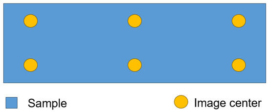
Figure 1.
Sample section with spots where images were taken.
2.2. Dataset
To obtain segments from steel images, unsupervised segmentation algorithms were considered. As a decision criterion, we wanted to use fast algorithms, preferably with O(N) computational complexity and with control over the number of clusters, without the need to perform complex image preprocessing steps prior to segmentation. Therefore, a Simple Iterative Linear Clustering (SLIC) was chosen, which adapts a k-means clustering approach to efficiently generate superpixels [21]. Its implementation from the sklearn library was employed. For each image, a distinct target number of segments was established (100, 400, and 600), and for each combination, the algorithm yielded a unique number of clusters.
Subsequently, a mask was generated for each segment. These masks were then combined with the original image through a process of arithmetic and operation, resulting in an intermediate image. The intermediate image was then cropped to remove any extraneous portions of the mask. The segments were stored individually and saved for each combination of original file and preset number of segments. We have noticed that higher compactness values led to more regular shapes of segments, but their boundaries were not matching with grains. Thus, compactness = 0.1 was used in this experiment.
In the second phase, manual labeling was performed on the previously prepared dataset to mark segments (See Figure 2) that contain small amounts of bainite, significant amounts of bainite, and no bainite. Segments that were difficult to classify were also marked and excluded from the dataset. Furthermore, classes of segments were binarized to predict presence or lack of bainite rather than its quantity. This allowed us to create a mapping between the segment image and its corresponding class. This approach was adopted to validate the correctness of the hypothesis. It draws from previous experiments where alternative methods, such as using the U-Net algorithm combined with Local Binary Patterns (LBPs), yielded inaccurate results. The decision to shift to this approach is based on observed limitations in earlier plans of experiments, emphasizing the need for a more robust and reliable solution to confirm selected features.
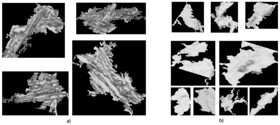
Figure 2.
Example of segments extracted from the image using superpixel segmentation. (a) Bainite segment. (b) Non-bainite segment. Original proportions were preserved.
Data preparation has been designed with the use of the medallion approach (it is a design of preparing data from the data engineering domain; see Figure 3), which allowed us to create a clean structure of the whole experiment.
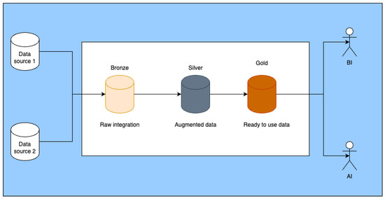
Figure 3.
Medalion data model.
The medallion model has been implemented with the use of 2 layers:
- The bronze layer;
- The silver layer.
The bronze layer is designed to store raw data described by metadata; in metadata, there is information about sources including date of update, etc. The silver layer is a place where the labeled data are stored for a given experiment. Every single experiment has its own preprocessing pipeline. So, the features are stored in separated places, but if some other experiments still need them, it is easy to find them. In Table 1 is the final number of prepared classes.

Table 1.
Number of final classes.
3. Algorithms
The algorithm was designed to operate on histograms. That is why we used an existing implementation of models and extended them with a new parameter, which is a BINS parameter. It helped us to define what number of bins the input histogram should have.
3.1. Tree Methods
In this approach, it has been decided to balance the input labels via reducing the number of samples with bainite. Thanks to that, the model was able to make sure that the final results show good metrics. This method used a decision tree algorithm and random forest algorithm.
Training
Input data have been split into train, validation, and test subsets with a random algorithm. There was no predefined rule, to make sure that the sets are not biased. They were split as follows:
- Training set → 60%;
- Validation set → 20%;
- Test set → 20%.
Training was based on grid search algorithm with cross-validation where the CV parameter equals 5. The decision tree hyperparameters were as follows:
- Histogram bins: [5, 10, 15, 20, 100, 150, 255];
- Criterion: [gini, entropy, log loss];
- Max depth: [None, 5, 10, 15, 20];
- Min samples split’: [2, 5, 10];
- Min samples leaf’: [1, 2, 5, 10].
The random forest hyperparameters were as follows:
- Histogram bins: [5, 10, 15, 20, 100, 150, 255];
- n estimators: [50, 100, 150];
- Criterion: [‘gini’, ‘entropy’];
- Max depth: [None, 5, 10, 15];
- Min samples split: [2, 5, 10];
- Min samples leaf: [1, 2, 5].
Table 2.
Number of final train classes.
Table 3.
Number of final validation classes.
Table 4.
Number of final test classes.
3.2. Hybrid Approach
In this section, a hybrid approach was utilized—unsupervised clustering to generate scarce data and supervised classification to evaluate how well the simple algorithm can perform classification. The data generation was decided due to imbalanced dataset and insufficient quantity of non-bainite segments.
3.2.1. K-Nearest Neighbors
The K-Nearest Neighbors (KNN) algorithm is one of the simplest algorithms belonging to the class of supervised machine learning algorithms. The classification is based on the majority of votes for the k most similar examples stored in the training set. Due to its simplicity, no extensive hyperparameter tuning is required [22,23].
3.2.2. K-Means
The goal of the k-means algorithm is to find k centers to minimize the sum of the squared distances between each point and its closest center (). Its simplicity and speed are very appealing in practice. Its basic formulation has been evolved by Arthur and Vassilvitskii in 2007 and presented as k-means++, for which the key objective was to improve accuracy and speed by a randomized seeding technique—choosing random starting centers with very specific probabilities [24].
3.3. Synthetic Histograms Generation and Classification
The Scikit-Learn v1.6.0 library implementation of KNN was used together with StratifiedShuffleSplit for 5 times Monte Carlo cross-validation. We considered k = 3, 5, 7, 9, 11, 13, and 15. Euclidean distance was used to assess similarity. Experiments wee performed on 5, 10, 15, 20, 100, 150, and 255 bins of the histogram. In total, 20% of the observations were moved to the test set and then the class proportions were balanced.
In contrast to the previous method, where excessive bainitic observations were pruned, this approach aims to retain them in the dataset by moving them from the test set to the training set to achieve equal class proportions in the test set. Synthetic non-bainitic segments were then generated using the k-means++ algorithm to cluster a subset of the training set consisting only of non-bainitic-like histograms. Different numbers of clusters (2–11) were tested to find the optimal configuration. The quality of each clustering is assessed by calculating the silhouette score, which measures how well the clusters are separated. The best number of clusters was selected based on the highest average silhouette score. Once optimal clusters were identified, the function generated new data by averaging histograms belonging to the same cluster and creating a desired, user-defined silhouette score. This approach ensured equal proportions in both the test and training sets, while maintaining control over the quality of the generated data through the application of a threshold to the silhouette for each data point (See Figure 4).
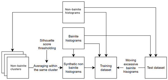
Figure 4.
Pipeline of the data processing for the KNN classification.
It is important to note that as the segment size increases, the generation of data based on high silhouette score observations becomes more challenging. Therefore, the following silhouette scores > 0.5 were used for images with fine- and medium-grained segments, Table 5 and Table 6 (600 and 400 segments set, respectively). For large-grained segments (100 segments set) several positive values were tested. Even the lowest value tested (0.1) was too high to generate a sufficient number of observations. We were therefore unable to classify large segments.
Table 5.
Number of final train classes.
Table 6.
Number of final test classes.
4. Results
4.1. Classification Results for Decision Tree
The results shown represent the optimal hyperparameter configurations for the selected initial segment values. The initial segment values are outlined below.
4.1.1. The Hyperparameter Settings and Results (Table 7) for the Given Initial Value of 600 Segments
Table 7.
DT results.
The best model was obtained for 5 bins of the histogram, entropy as a criterion, max depth 15, min samples split 10, and min samples leaf 5.
4.1.2. The Hyperparameter Settings and Results (Table 8) for the Given Initial Value of 400 Segments
Table 8.
DT-400 results.
The best model was obtained for 10 bins of the histogram, gini as a criterion, max depth none, min samples split 2, and min samples leaf 10.
4.1.3. The Hyperparameter Settings and Results (Table 9) for the Given Initial Value of 100 Segments
Table 9.
DT-100 results.
The best model was obtained for 5 bins of the histogram, gini as a criterion, max depth none, min samples split 5, and min samples leaf 2.
As we can see, those values are very unstable. The main problem is with the small number of classes in those datasets. The model is not able to detect the features. It only tries to match the exact results from the training set (the parameter none in max depth can suggest that this model is over-trained).
4.2. Classification Results for Random Forest
There are further results for the best hyperparameters for chosen segments’ initial values.
4.2.1. The Hyperparameter Settings and Results (Table 10) for the Given Initial Value of 600 Segments
Table 10.
RF-600 results.
The best model was obtained for 100 bins of the histogram, entropy as a criterion, max depth 10, min samples split 10, min samples leaf 1, and n estimators 50.
4.2.2. The Hyperparameter Settings and Results (Table 11) for the Given Initial Value of 400 Segments
Table 11.
RF-400 results.
The best model was obtained for 5 bins of the histogram, entropy as a criterion, max depth 10, min samples split 5, min samples leaf 1, and n estimators 50.
4.2.3. The Hyperparameter Settings and Results (Table 12) for the Given Initial Value of 100 Segments
Table 12.
RF-100 results.
The best model was obtained for 5 bins of the histogram, gini as a criterion, max depth none, min samples split 5, min samples leaf 1, and n estimators 50.
4.3. Classification Results for K-Nearest Neighbors
4.3.1. The Hyperparameter Settings and Results (Table 13) for the Given Initial Value of 600 Segments
Table 13.
KNN-600 results.
The best model was obtained for 5 bins of the histogram and k = 5.
4.3.2. The Hyperparameter Settings and Results (Table 14) for the Given Initial Value of 400 Segments
Table 14.
KNN-400 results.
The best model was obtained for 150 bins of the histogram and k = 11.
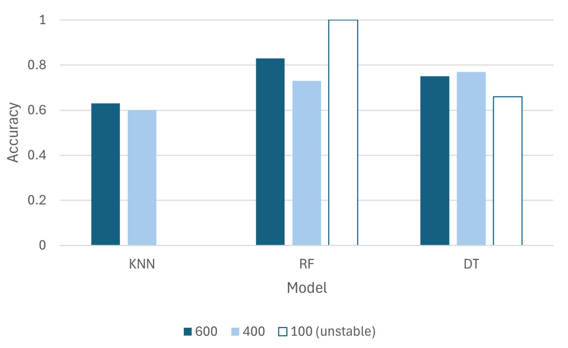
As illustrated in Figure 5, the accuracy of all models is presented. It should be noted that for the dataset composed of large segments, the accuracy is high. However, different metrics indicated unreliability, and thus, these results were marked as unstable.

Figure 5.
Summary of model performance for different numbers of segments.
5. Discussion
The findings highlight the significant challenges associated with applying machine learning techniques to bainite recognition in steel microstructures. Among the tested approaches, the random forest algorithm delivered the best overall performance; however, its dependence on engineered features derived from histogram data constrains its ability to adapt to more intricate image characteristics. This limitation underscores the importance of exploring advanced deep learning methods, such as CNNs, which excel at automatically extracting features directly from raw image data. Additionally, it is essential to evaluate algorithms capable of generating or incorporating novel features to enhance model robustness.
The current study involves a broad range of tested parameters. It is important to note that these models are not typically used in conventional image analysis. However, the primary objective of this paper is to highlight that the selected application—histogram analysis—has the potential to provide new features for more advanced models. These features could assist in reducing the search space for future parameter optimization, particularly in models such as CNNs that need much more computational capacity than the presented methods.
The analysis also revealed that datasets that comprise large segments yielded inconsistent and unstable results. An increase in the segment area corresponds to a decrease in the size of the dataset. The suboptimal performance of the model for small datasets is attributable to more than just the limited size of the datasets. Large segments covered a greater sample area by encompassing a broader spectrum of microstructures. In such instances, the binary classification of segments becomes challenging. As the volume of data to be analyzed by the expert increases, the decision boundary becomes less distinct, and rudimentary image analysis techniques, such as the histogram, may not adequately reflect the characteristics of the heterogeneous microstructure. Given the previously indicated characteristics of large segments, increasing the amount of data in the datasets by generating them or applying augmentation using only histograms may not result in a significant improvement in model performance. Potential solutions include the extraction of additional, more descriptive features of the segments, based on which it will be possible to classify them more accurately, but further investigation is needed in the context of segment size optimization. This study also emphasizes the need to implement more rigorous cross-validation strategies. These strategies are necessary to ensure robust performance evaluations.
Classification based on histograms has a higher explanatory power than when using black-box models, such as CNNs. The proposed method is conducive to the creation of a knowledge base that can be used to accelerate and improve the quality of the microstructure analysis process in the industry. However, reliance on histogram bins as the primary features for classification may overlook critical spatial and textural details that are fundamental to accurately distinguishing bainite from other microstructural components. To address these shortcomings, future research should prioritize feature extraction techniques [2] capable of capturing the nuanced patterns present in microstructural images. This could involve integrating spatial context, texture analysis, and advanced machine learning frameworks to achieve more reliable and accurate bainite classification.
This study demonstrated the feasibility of providing potential support for experts in the sample validation process. This support could result in more consistent validation results and a reduction in the time necessary to analyze samples.
6. Conclusions
This study aimed to enhance bainite recognition in steel microstructures using machine learning techniques. By applying unsupervised segmentation (SLIC) and supervised classification methods (decision trees, random forests, and KNN), the authors evaluated their effectiveness in identifying bainitic regions. Results for smaller datasets (100 segments set, large segment area) were unstable, with limited generalizability.
Increasing the number of segments improved model stability, while splitting images into smaller segments and analyzing histograms proved viable for bainite detection. However, this approach may overlook critical spatial and textural details. Future efforts should focus on neural networks capable of extracting advanced features from raw image data and generating metadata to quantify bainite and non-bainite regions. Smaller datasets yielded unstable results, emphasizing the importance of larger datasets and robust validation.
Author Contributions
Conceptualization, T.J., F.H. and K.R.; Data curation, G.K.; Funding acquisition, K.R.; Investigation, T.J. and F.H.; Methodology, T.J. and F.H.; Project administration, K.R.; Resources, G.K.; Software, T.J. and F.H.; Supervision, K.R.; Validation, T.J. and F.H.; Writing—original draft, T.J. and F.H.; Writing—review and editing, G.K. and K.R. All authors have read and agreed to the published version of the manuscript.
Funding
This study was carried out as part of the fundamental research financed by the Ministry of Science and Higher Education, grant no. 16.16.110.663.
Institutional Review Board Statement
Not applicable.
Informed Consent Statement
Not applicable.
Data Availability Statement
The original contributions presented in this study are included in the article. Further inquiries can be directed to the corresponding author.
Conflicts of Interest
The authors declare no conflicts of interest.
References
- Bhadeshia, H.K.D.H.; Christian, J.W. Bainite in Steels. Metall. Trans. A 1990, 21, 767–797. [Google Scholar] [CrossRef]
- Gola, J.; Britz, D.; Staudt, T.; Winter, M.; Schneider, A.S.; Ludovici, M.; Mücklich, F. Advanced microstructure classification by data mining methods. Comput. Mater. Sci. 2018, 148, 324–335. [Google Scholar] [CrossRef]
- Muñoz-Rodenas, J.; García-Sevilla, F.; Miguel-Eguía, V.; Coello-Sobrino, J.; Martínez-Martínez, A. A Deep Learning Approach to Semantic Segmentation of Steel Microstructures. Appl. Sci. 2024, 14, 2297. [Google Scholar] [CrossRef]
- Ackermann, M.; Iren, D.; Wesselmecking, S.; Shetty, D.; Krupp, U. Automated segmentation of martensite-austenite islands in bainitic steel. Mater. Charact. 2022, 191, 112091. [Google Scholar] [CrossRef]
- Directorate-General for Research and Innovation (European Commission); Zajac, S.; Morris, P.; Komenda, J. Quantitative Structure-Property Relationships for Complex Bainitic Microstructures—Final Report; Publications Office: Brussels, Belgium, 2005. [Google Scholar]
- Müller, M.; Britz, D.; Ulrich, L.; Staudt, T.; Mücklich, F. Classification of Bainitic Structures Using Textural Parameters and Machine Learning Techniques. Metals 2020, 10, 630. [Google Scholar] [CrossRef]
- Gola, J.; Webel, J.; Britz, D.; Guitar, A.; Staudt, T.; Winter, M.; Mücklich, F. Objective microstructure classification by support vector machine (SVM) using a combination of morphological parameters and textural features for low carbon steels. Comput. Mater. Sci. 2019, 160, 186–196. [Google Scholar] [CrossRef]
- Tsutsui, K.; Terasaki, H.; Maemura, T.; Hayashi, K.; Moriguchi, K.; Morito, S. Microstructural diagram for steel based on crystallography with machine learning. Comput. Mater. Sci. 2019, 159, 403–411. [Google Scholar] [CrossRef]
- Komenda, J. Automatic recognition of complex microstructures using the Image Classifier. Mater. Charact. 2001, 46, 87–92. [Google Scholar] [CrossRef]
- Miyama, E.; Voit, C.; Pohl, M. Zementitnachweis zur Unterscheidung von Bainitstufen in modernen, niedriglegierten Mehrphasenstählen. Pract. Metallogr. 2011, 48, 261–272. [Google Scholar] [CrossRef]
- Banerjee, S.; Datta, S.; Paul, B.; Saha, S.K. Segmentation of three phase micrograph: An automated approach. In Proceedings of the CUBE International Information Technology Conference—CUBE ’12, New York, NY, USA, 3–6 September 2012; pp. 1–4. [Google Scholar] [CrossRef]
- Paul, A.; Gangopadhyay, A.; Chintha, A.R.; Mukherjee, D.P.; Das, P.; Kundu, S. Calculation of phase fraction in steel microstructure images using random forest classifier. IET Image Process. 2018, 12, 1370–1377. [Google Scholar] [CrossRef]
- Ronneberger, O.; Fischer, P.; Brox, T. U-Net: Convolutional Networks for Biomedical Image Segmentation. In Proceedings of the Medical Image Computing and Computer-Assisted Intervention—MICCAI 2015; Navab, N., Hornegger, J., Wells, W.M., Frangi, A.F., Eds.; Springer: Cham, Switzerland, 2015; pp. 234–241. [Google Scholar]
- Wood, G.A. Quality Control in the Hard-Metal Industry. Powder Metall. 1970, 13, 338–365. [Google Scholar] [CrossRef]
- Schneider, J.; Rostami, R.; Corcoran, M.; Korpala, G. Integration of Artificial Intelligence into Metallography: Area-wide Analysis of Microstructural Components of a Jominy Sample. HTM J. Heat Treat. Mater. 2024, 79, 3–14. [Google Scholar] [CrossRef]
- Breiman, L.; Friedman, J.; Olshen, R.A.; Stone, C.J. Classification and Regression Trees, 1st ed.; Chapman and Hall/CRC: Boca Raton, FL, USA, 1984. [Google Scholar]
- Baran, W.; Regulski, K.; Milenin, A. Influence of Materials Parameters of the Coil Sheet on the Formation of Defects during the Manufacture of Deep-Drawn Cups. Processes 2022, 10, 578. [Google Scholar] [CrossRef]
- Biau, G.; Scornet, E. A random forest guided tour. Test 2016, 25, 197–227. [Google Scholar] [CrossRef]
- Pedregosa, F.; Varoquaux, G.; Gramfort, A.; Michel, V.; Thirion, B.; Grisel, O.; Blondel, M.; Prettenhofer, P.; Weiss, R.; Dubourg, V.; et al. Scikit-learn: Machine Learning in Python. J. Mach. Learn. Res. 2011, 12, 2825–2830. [Google Scholar]
- Yu, Y.; Yao, M. When Convolutional Neural Networks Meet Laser-Induced Breakdown Spectroscopy: End-to-End Quantitative Analysis Modeling of ChemCam Spectral Data for Major Elements Based on Ensemble Convolutional Neural Networks. Remote Sens. 2023, 15, 3422. [Google Scholar] [CrossRef]
- Achanta, R.; Shaji, A.; Smith, K.; Lucchi, A.; Fua, P.; Süsstrunk, S. SLIC Superpixels Compared to State-of-the-Art Superpixel Methods. IEEE Trans. Pattern Anal. Mach. Intell. 2012, 34, 2274–2282. [Google Scholar] [CrossRef] [PubMed]
- Tomat, A. Interval pattern structures for interpreting K-nearest neighbor approach in lazy classification. In Proceedings of the 11th International Workshop “What Can FCA Do for Artificial Intelligence?”, FCA4AI 2023, Co-Located with IJCAI 2023, Macao, China, 20 August 2023; pp. 17–24.
- Changjun, Z.; Yuzong, C. The Research of Vehicle Classification Using SVM and KNN in a Ramp. In Proceedings of the 2009 International Forum on Computer Science-Technology and Applications, Chongqing, China, 25–27 December 2009; Volume 3, pp. 391–394. [Google Scholar] [CrossRef]
- Arthur, D.; Vassilvitskii, S. K-means++: The advantages of careful seeding. In Proceedings of the Eighteenth Annual ACM-SIAM Symposium on Discrete Algorithms, New Orleans, LA, USA, 7–9 January 2007; pp. 1027–1035. [Google Scholar]


Disclaimer/Publisher’s Note: The statements, opinions and data contained in all publications are solely those of the individual author(s) and contributor(s) and not of MDPI and/or the editor(s). MDPI and/or the editor(s) disclaim responsibility for any injury to people or property resulting from any ideas, methods, instructions or products referred to in the content. |
© 2025 by the authors. Licensee MDPI, Basel, Switzerland. This article is an open access article distributed under the terms and conditions of the Creative Commons Attribution (CC BY) license (https://creativecommons.org/licenses/by/4.0/).