Research on Damage Detection Methods for Concrete Beams Based on Ground Penetrating Radar and Convolutional Neural Networks

Abstract

Ground penetrating radar (GPR) is a mature and important research method in the field of structural non-destructive testing. However, when the detection target scale is small and the amount of data collected is limited, it poses a serious challenge for this research method. In order to verify the applicability of typical one-dimensional radar signals combined with convolutional neural networks (CNN) in the non-destructive testing of concrete structures, this study created concrete specimens with embedded defects (voids, non-dense solids, and cracks) commonly found in concrete structures in a laboratory setting. High-frequency GPR equipment is used for data acquisition, A-scan data corresponding to different defects is extracted as a training set, and appropriate labeling is carried out. The extracted original radar signals were taken as the input of the CNN model. At the same time, in order to improve the sensitivity of the CNN models to specific damage types, the spectrums of A-scan are also used as part of the training datasets of the CNN models. In this paper, two CNN models with different dimensions are used to train the datasets and evaluate the classification results; one is the traditional one-dimensional CNN model, and the other is the classical two-dimensional CNN architecture AlexNet. In addition, the finite difference time domain (FDTD) model of three-dimensional complex media is established by gprMax, and the propagation characteristics of GPR in concrete media are simulated. The results of applying this method to both simulated and experimental data show that combining the A-scan data of ground penetrating radar and their spectrums as input with the CNN model can effectively identify different types of damage and defects inside the concrete structure. Compared with the one-dimensional CNN model, AlexNet has obvious advantages in extracting complex signal features and processing high-dimensional data. The feasibility of this method in the research field of damage detection of concrete structures has been verified.

1. Introduction

With the continuous deepening of interdisciplinary research, the civil engineering industry is developing towards a more efficient, intelligent, and sustainable direction. As one of the most common building materials, the safety and durability of concrete structures are crucial for ensuring the safety of people’s lives and property. However, long-term exposure to complex and changing environmental conditions makes concrete structures susceptible to various damages such as corrosion, cracks, and voids. These damages not only weaken the load-bearing capacity of the structure but may also cause serious safety accidents. Therefore, timely and accurate detection of internal damage in concrete structures is of great significance for preventing disasters and extending the service life of structures [1]. Traditional concrete structure detection methods, such as drilling sampling and tapping detection [2], can provide information on the structural state to a certain extent but often come with damage to the structure, low detection efficiency, and high cost. In recent years, non-destructive testing technology [3,4,5,6] has gradually become a research hotspot in the field of concrete structure testing due to its non-destructive, efficient, and accurate characteristics. Among them, Ground Penetrating Radar (GPR) technology, with its unique electromagnetic wave detection principle, has shown great potential in-depth detection, defect identification, and localization of concrete structures. GPR technology achieves “perspective” detection of the internal conditions of concrete structures by emitting high-frequency electromagnetic wave pulses and receiving signals reflected back from different medium interfaces inside the structure. This technology can identify key information such as cracks, voids, and steel bar distribution in concrete, as well as provide high-resolution two-dimensional or three-dimensional image data without affecting structural integrity, providing strong technical support for structural health monitoring and evaluation.

The GPR system consists of one or more transmitting and receiving antennas. As shown in Figure 1. The transmitting antenna sends high-frequency electromagnetic pulses into the subsurface, typically in the frequency range of several hundred megahertz to several thousand megahertz. When electromagnetic waves encounter underground materials with different dielectric constants such as soil, rock, water, metals, etc., they will be reflected and refracted. The variation in dielectric constant is usually related to the composition, moisture content, and density of the material. The receiving antenna captures the reflected electromagnetic wave signal. The intensity and propagation time of reflected signals provide information about the size, shape, and location of underground objects [7]. Data can be converted into images through display systems or computer software.

At present, in the existing application research in the civil engineering industry, GPR has been used to assess pavement thickness or pavement delamination [8,9], to detect internal structural detachment, and to identify buried objects, among others. In bridge surveys, GPR is used to evaluate concrete bridge decks [10] and to provide an assessment based on the corrosion condition of reinforced concrete deck slabs [11,12], among others. In tunneling, the lining plays a vital role in maintaining the stability of the tunnel by withstanding the pressure of the surrounding rock and the self-weight of the structure [13]. GPR is used to check the quality and integrity of the lining structure, detecting defects, voids, and contact with the surrounding rock in a non-contact manner. The technique helps to identify potential problems in advance and improves the safety of the project.

Deep learning is expected to play a greater role in civil engineering as algorithms continue to evolve and data acquisition methods advance. Convolutional neural networks (CNNs), the core foundation of deep learning, can learn low-level features (such as edges and textures) to high-level features (such as shapes and object parts). This hierarchical feature abstraction allows CNNs to excel at visual tasks and effectively extract high-dimensional image features [14], which has become the mainstream image processing technology in the field of computer vision. Neural networks and deep learning techniques have been widely used in many aspects of civil engineering [15,16,17]. For example, Xue and Li [18] proposed a full convolutional neural network-based approach for classifying and recognizing various defects on the external surface of tunnel linings. They verified that this model outperforms several other convolutional neural network models (e.g., AlexNet, GoogLeNet, and Visual Geometry Group network-16) in terms of performance, exhibiting higher accuracy and faster processing speed. Zhou et al. [19] proposed an enhanced YOLO v4 model for high-precision real-time detection and identification of various defects in tunnel linings. These studies have realized damage recognition and classification to a certain extent, but most of the data sets used rely on regional images captured by high-definition cameras, and damage recognition and classification are mainly based on whether there are defects in the images. Although surface defects in buildings can be easily identified, internal defects within the structure are often undetectable, which limits the comprehensiveness and accuracy of damage assessment. Vibration signals, by monitoring the structural vibrations under different loads and environmental conditions, can provide information about the internal state of the structure. Subtle internal defects typically affect the dynamic response characteristics of the structure, such as natural frequencies and mode shapes [20]. These changes can be detected and evaluated by accurately analyzing vibration signals, which can reveal internal damage rather than relying solely on surface images [21,22,23]. However, while the vibration signal primarily reflects the damage condition through the structural vibration characteristics, the process of achieving internal imaging of the structure is more complex. Internal imaging provides a more intuitive overview and comprehensive information about the internal state of the structure, effectively identifying potential internal defects such as cracks, voids, and reinforcement corrosion.

As an important branch of deep learning, CNN has been mainly applied to the sequence feature extraction of 2D and 3D images in recent years [24]. Some scholars have introduced CNN into the field of GPR and efficiently achieved the detection, identification, and classification of internal defects in concrete structures by combining GPR and CNN [25]. Zhang et al. [26] used the proposed IRS method to generate suitable images from collected GPR data and feed them to CNN to detect and accurately locate water damage on asphalt concrete pavement. In order to quickly, accurately, and automatically detect the target signals in the GPR image, Gao et al. [27] proposed an improved speed-RCNN algorithm for GPR pavement detection, which achieved considerable accuracy in detecting cracks, water damage pits, and uneven settlement. Although the above examples demonstrate successful experiments of deep learning in certain ground-penetrating radar scenarios, there are still some challenges in practical field applications. On the one hand, due to the scarcity of defect data in the acquired GPR data, it is essential to collect a sufficiently rich set of ground-penetrating radar images to support the training of supervised deep learning models. Moreover, the cost of labeling many GPR image samples containing defects is high because the labeling process is time-consuming, labor-intensive, and relies on professional knowledge. The radar signal (A-scan), as a typical one-dimensional time-domain signal, provides key information about the position, shape, and material properties of the target object through amplitude and phase information at each time point [28]. Therefore, it is particularly important to effectively process and analyze these signals. Xu et al. [29] proposed an adaptive one-dimensional convolutional neural network (one-dimensional) algorithm applied to GPR data, which successfully classified different types of damaged road surfaces. Li et al. [30] used YOLO v3 to automatically recognize the signals reflected by rebars in GPR images and accurately estimated the thickness of the protective layer and the diameter of the rebar by using one-dimensional. This indicates that one-dimensional can effectively capture local features in radar A-scan and automatically learn the important features in the signal, thereby effectively classifying different types of damage. In practical applications, using CNN to analyze A-scan data can improve the detection accuracy of potential structural defects. In addition, the adaptive nature of the method enables it to adapt to various signal patterns and environmental conditions, providing strong support for more intelligent and automated structural health monitoring.

Based on the characteristics of GPR data and the theoretical basis of one-dimensional and two-dimensional CNN, this paper explores the training process and classification results of different types of defects in small-scale concrete structures using one-dimensional A-scan radar signals and corresponding two-dimensional spectrums as input data, and evaluate the datasets using CNN models. In Section 2, we introduced the theoretical basis of one-dimensional CNN and classical two-dimensional CNN architecture AlexNet. In Section 3, gprMax was used to simulate three-dimensional complex reinforced concrete beams with built-in defects. At the same time, three sets of concrete beam parameters and experimental processes used in laboratory experiments were introduced.

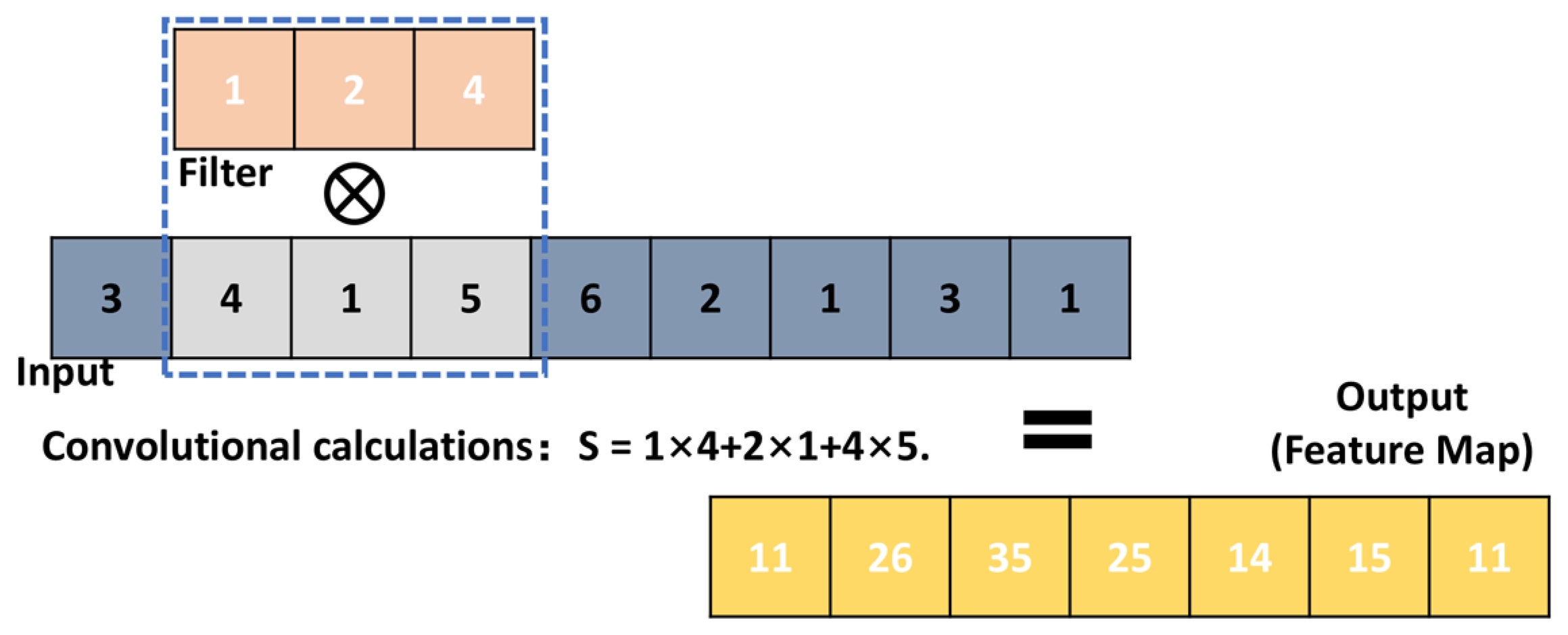
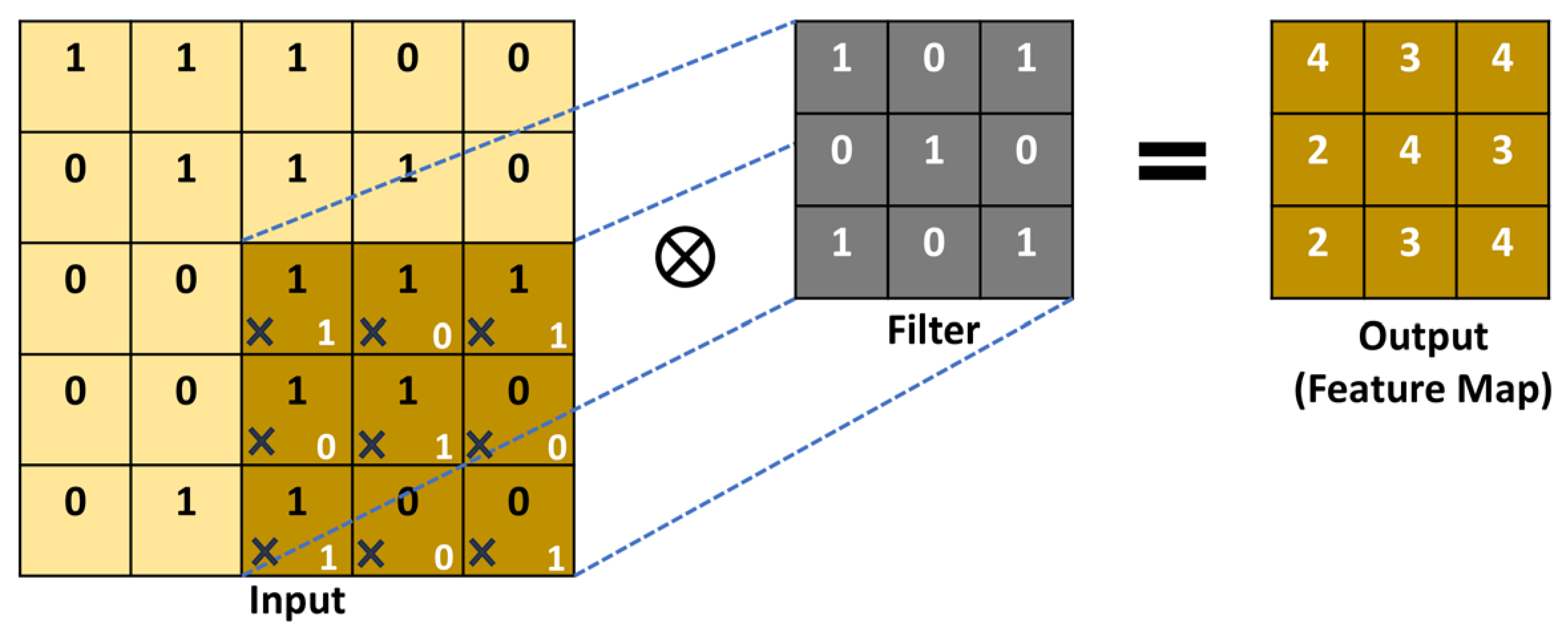
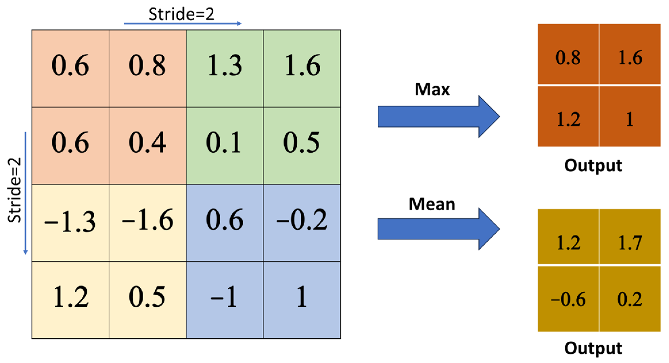
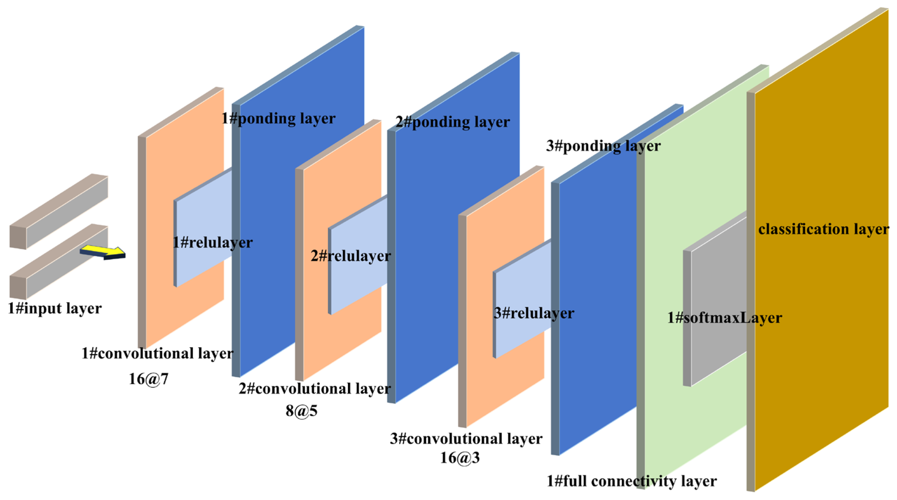
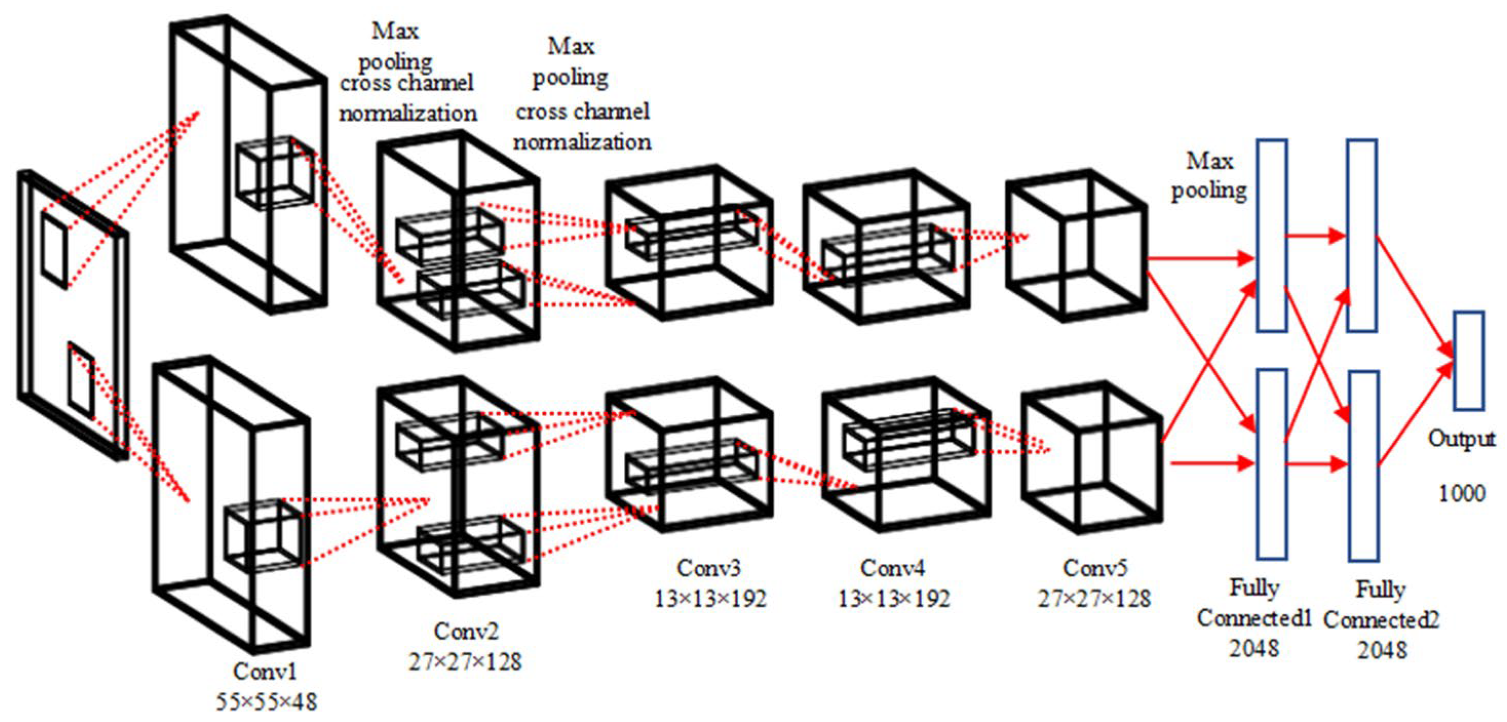
2. Architecture of the CNNs

Convolutional neural networks (CNNs) are typical multilayer nonlinear feedforward neural networks originally designed for feature extraction and recognition of complex images, demonstrating superior nonlinear representation capabilities. The core component of a CNN model is the convolutional layer. Each convolutional block contains learnable parameters such as weights (filters) and biases. The filters are usually smaller in width and height compared to the input, but their depth is the same as that of the input layer. The feature map of the previous layer is convolved with the filter through an activation function to generate the output. The calculation between the pixels in the convolution layer can be expressed as follows:

$${\mathrm{C}}_{\mathrm{x}\mathrm{y}}=\mathsf{\sigma }\left(\sum _{\mathrm{i}=1}^{\mathrm{h}}{\sum }_{\mathrm{j}=1}^{\mathrm{w}}{\sum }_{\mathrm{k}=1}^{\mathrm{d}}{\mathrm{f}}_{\mathrm{i}\mathrm{j}\mathrm{k}}\mathrm{\ast }{\mathrm{X}}_{\mathrm{x}+\mathrm{i},\mathrm{y}+\mathrm{j}-1,\mathrm{k}}+\mathrm{b}\right)$$

(1)

where $\mathrm{h}$ and $\mathrm{w}$ are the sizes of the filter, and d is the number of channels of the input, $\mathrm{x},\mathrm{y}$ is the input vector, $\mathrm{b}$ is the bias vector, $\mathsf{\sigma }$ is the activation function, and f is the weight matrix. Figure 2 shows the operation of a one-dimensional convolution of an input random sequence. The convolution kernel of a one-dimensional convolution is a one-dimensional array, such as using a convolution kernel of length that slides over one dimension, multiplying and summating each time with a point on the current sequence.

The convolution kernel of a two-dimensional convolution slides simultaneously in both dimensions’ height and width. Figure 3 shows the convolution operation on a randomly selected 5 × 5 matrix. A 3 × 3 matrix is selected as the filter, which is randomly generated in the initial state and updated from the model by backpropagation algorithm.

The convolutional layer is followed by a nonlinear activation function, which is used to introduce nonlinearity in the network. The two most commonly used activation functions in neural networks are rectified linear unit ReLU and softmax. In this article, the one-dimensional convolutional neural network and the two-dimensional convolutional neural network used Softmax and ReLU as activation functions, respectively. The functional representation of ReLU and Softmax is given, respectively, as follows:

$$\mathrm{f}\left(\mathrm{x}\right)=\max \left(0,\mathrm{x}\right)$$

(2)

$${\mathrm{f}\left(\mathrm{x}\right)}_{\mathrm{i}}={\displaystyle \frac{{\mathrm{e}}^{\mathrm{x}\mathrm{i}}}{\sum _{\mathrm{j}=1}^{\mathrm{K}}{\mathrm{e}}^{\mathrm{x}\mathrm{j}}}}$$

(3)

The purpose of the pooling layer is to reduce the spatial size of the feature map, thereby speeding up computation and enhancing the robustness of feature detection. Common pooling methods include max pooling and average pooling. In max pooling, the maximum value from the filtering region is selected as the output. For instance, as shown in Figure 4, a 4 × 4 input layer is processed using a 2 × 2 max pooling filter. The stride is set to 2, which means that the next filter will move two positions to the right and downward, resulting in an output dimension of 2 × 2, where the values correspond to the maximum elements from the receptive fields. In average pooling, on the other hand, the average value within the filter region is computed as the output.

The fully connected layer is the last right before the output layer of the network. In this layer, all neurons are connected to the features generated by the previous layer. The weights and biases of this layer are responsible for transforming these features into the corresponding classes. The equation for the output ${\mathrm{y}}^{\mathrm{l}}$ is shown as follows:

$${\mathrm{y}}^{\mathrm{l}}=\mathsf{\sigma }\left({\mathrm{y}}^{\mathrm{l}-1}\mathrm{\ast }\mathrm{w}+\mathrm{b}\right)$$

(4)

where $\mathsf{\sigma }$ is the activation function; $\mathrm{w}$ and $\mathrm{b}$ represent the weights and bias vectors in this layer, respectively.

The one-dimensional model in this article comprises three convolutional layers, three pooling layers, and one fully connected layer. A max pooling layer with a size of three is placed between every two consecutive convolutional layers to reduce data redundancy and mitigate the risk of overfitting. The framework of the one-dimensional neural network is shown in Figure 5. The 2D convolutional neural network model used in this paper is AlexNet [14], AlexNet has excellent image classification performance. AlexNet is a huge network with 60 million parameters and 650,000 neurons. The AlexNet has eight layers. Its first five layers are convolutional layers, and the last three layers are fully connected (See Figure 6). In this paper, the input data type for the one-dimensional model is a one-dimensional array, while the input data type for the two-dimensional model is a 227 × 227 image. The outputs of both models are different types of damage categories.

3. Numerical Simulation and Laboratory Testing

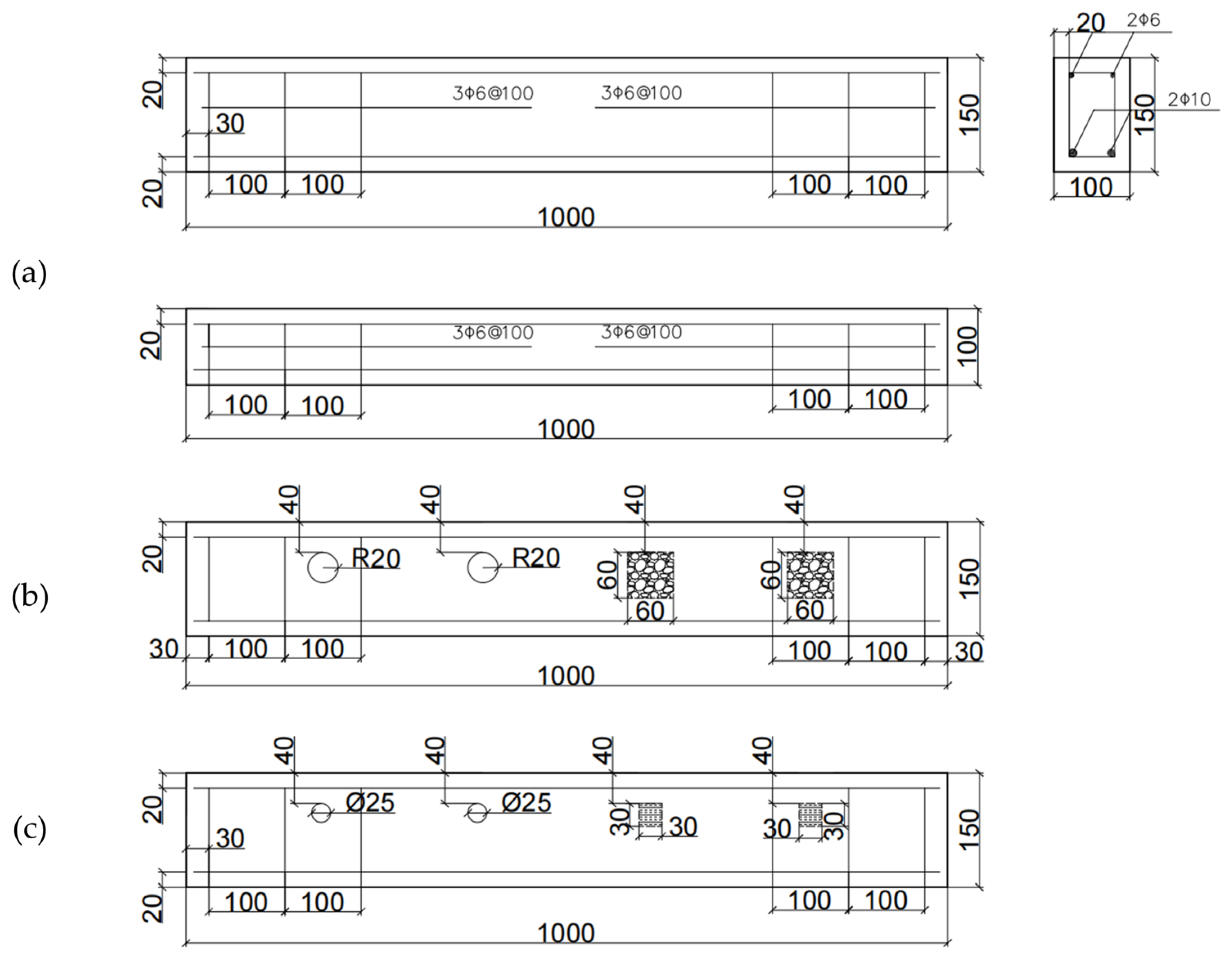
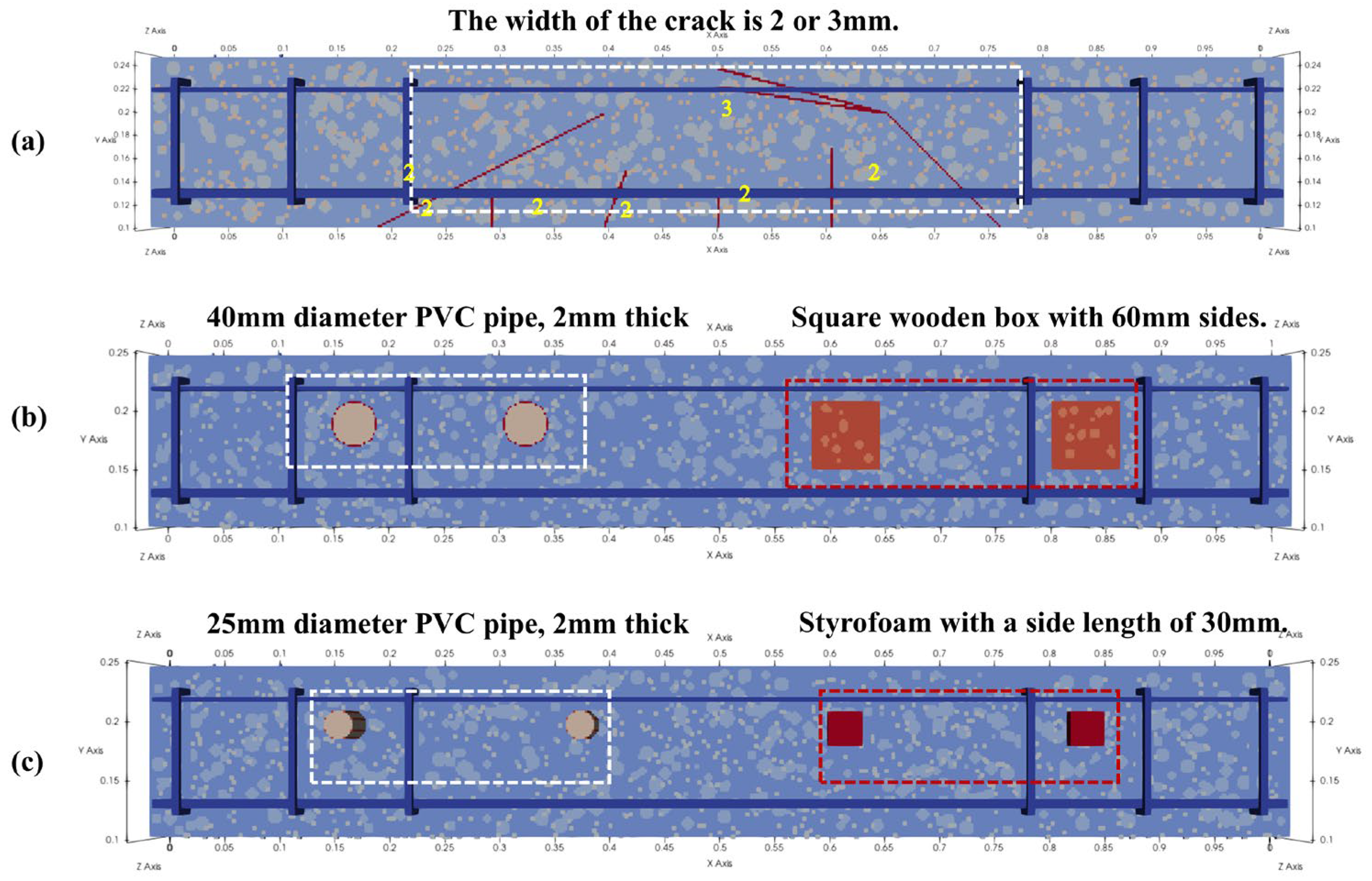
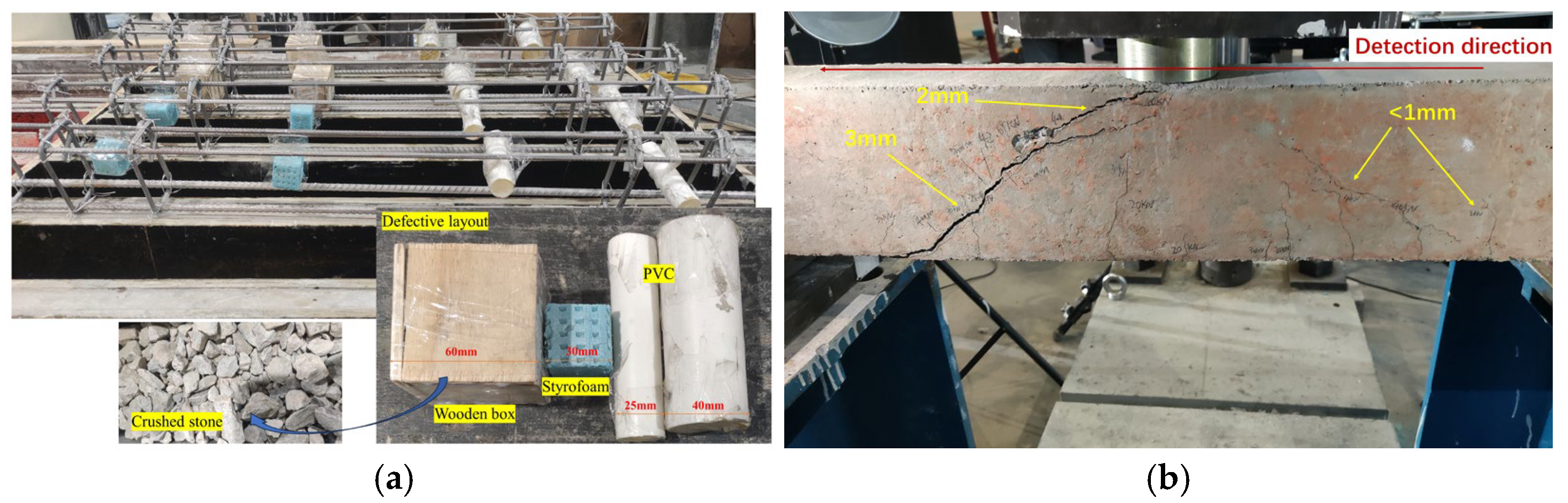
3.1. Design of Concrete Beams with Defects

In this study, several defects that may occur in concrete beams, such as voids, impermeable solids, and cracks, were considered. Different sizes of polyvinyl chloride pipes, polystyrene foam, and square wooden boxes containing slurry-free gravel were selected to simulate voids and impermeable solids of different sizes, respectively, and cracks were simulated from a set of simply supported reinforced concrete beam bending tests. In order not to influence each other’s test results, the defects were set at a certain distance from each other, and each beam was numbered with the specific information shown in

Table 1. Concrete beam defect information and measurement methods.

Information	Number	Defective Layout	Measurement Method	Strength & Dimensions
(a)	H_B0	-	scan after loading	Strength: C30 Dimensions: 1000 × 150 × 100 mm
(b)	H_BF1	PVC, Wooden box	Direct scan
(c)	H_BF2	PVC, Styrofoam	Direct scan

. The defect layout and reinforcement of the concrete beams are shown in Figure 7.

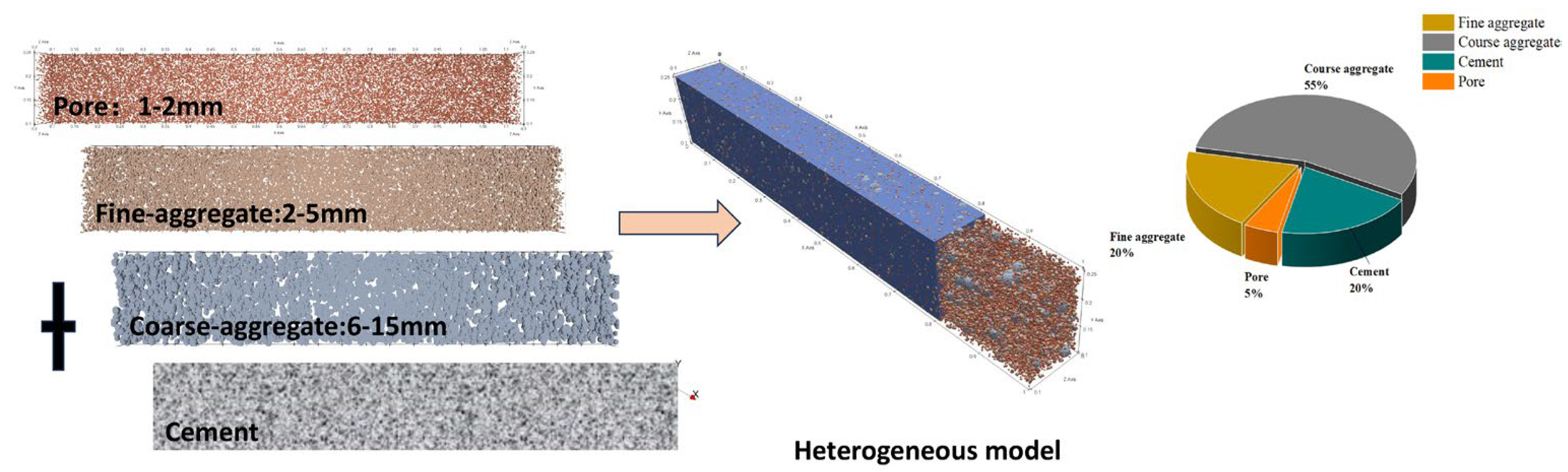
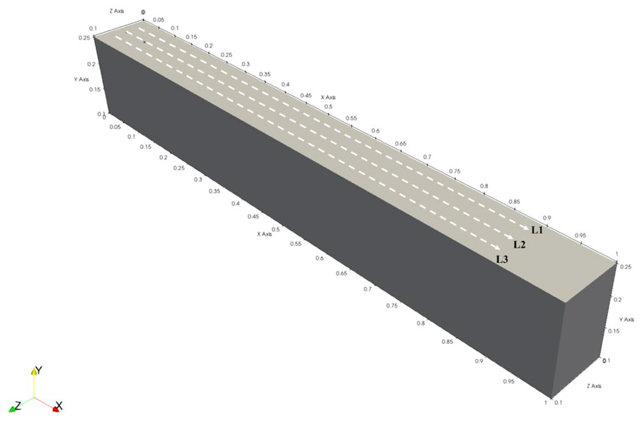
3.2. Numerical Simulation

Concrete, as a typical composite material, has a high degree of non-uniformity, and changes in its internal structure can significantly affect its dielectric properties. The different components of concrete (such as cement, aggregates, additives, etc.) have different dielectric constants, and changes in the proportion of components can lead to changes in the overall dielectric constant [31,32]. Therefore, it is crucial to develop more accurate and heterogeneous electromagnetic field propagation material models [33]. This article proposes a three-dimensional numerical model of heterogeneous concrete (See Figure 8), where the distribution of different materials in concrete is random. By writing Python scripts, the specific positions of different materials in concrete structures are randomly generated. In the model, materials such as coarse aggregate, fine aggregate, and cement are defined, and they have different volume fractions and particle size ranges in concrete. For example, the particle size of coarse aggregate is greater than or equal to 5 mm, while the particle size of fine aggregate is between 1 mm and 5 mm. In addition, each material is assigned different dielectric parameters, and after setting the aggregate parameters, the remaining space in the concrete model is filled with cement material. This script is implemented in the input file of gprMax [34,35].

The specific internal material parameters of concrete are shown in

Table 2. Material properties in 3D models.

Materials	Dielectric Constant	Electric Conductivity	Relative Permeability	Magnetic Loss	Volume Proportion	Particle Size (mm)
Coarse aggregate	7.0	0	1.0	0	55%	6–20
Fine aggregate	6.0	0	1.0	0	20%	2–5
Cement	6.5	0	1.0	0	20%	-
Air	1.0	0	1.0	0	5%	2

, and the internal material information of concrete is shown in

Table 3. Parameters of build-in materials in concrete beams.

Defective Material	Dielectric Constant	Size
PVC	4	Diameter size: 40 mm, 25 mm
Wooden box	2.5	Length: 60 mm
Crushed stone	7	-
Styrofoam	3	Length: 30 mm

.

The thickness of PVC pipes and square wooden boxes in the model with built-in defects is 2 mm, and the concrete beam model with built-in defects is shown in Figure 9. We divided three sampling lines, L1, L2, and L3, on the surface of each concrete beam (see Figure 10). Due to the unevenness inside the concrete, the A-scans of L1, L2, and L3 are not the same in the cross-section of the concrete structure. Therefore, collecting multiple measurement lines ensures the repeatability of the data and enrich the datasets available for training CNN models.

Table 4. Numerical simulation parameter settings.

Parameters	Specified Value
domain	1.000 0.150 0.100
dx_dy_dz	0.002
time_window	5 × 10−9
waveform	Ricker, 1.6 GHz
hertzian_dipole	0.056 0.250 0.050
rx	0.114 0.250 0.050
steps	0.004

shows the parameter settings for the gprMax 3.0 orthotropic simulation. The size of the meshes delineated is 0.002 × 0.002 × 0.002 m. The parameter settings for the numerical simulation of all three concrete beams are the same, differing in the internal morphology of the concrete.

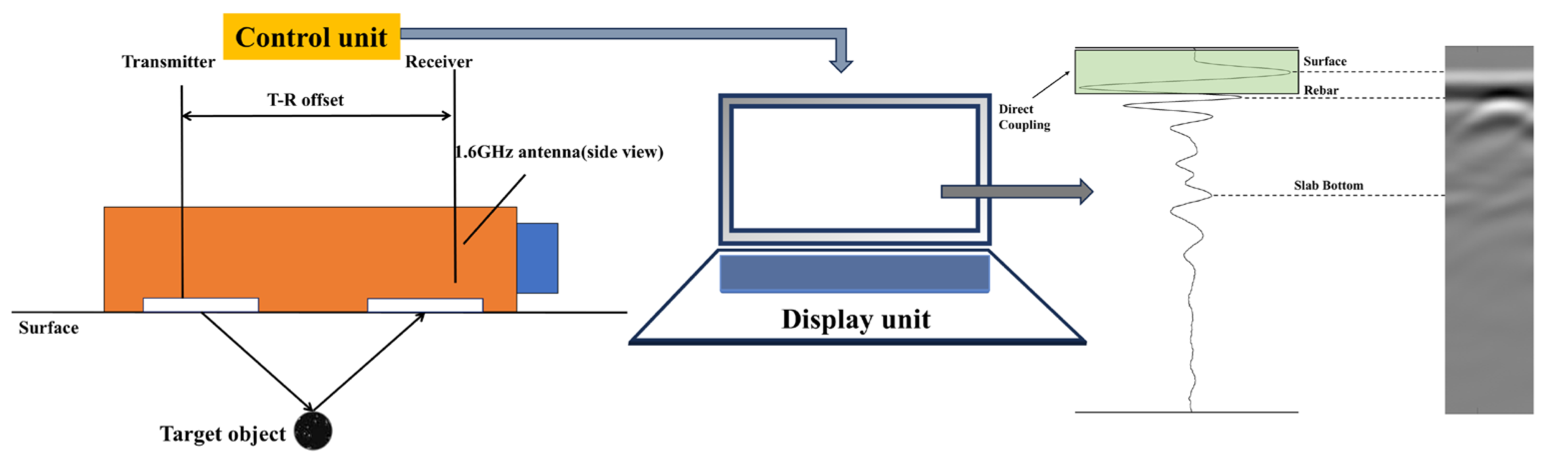
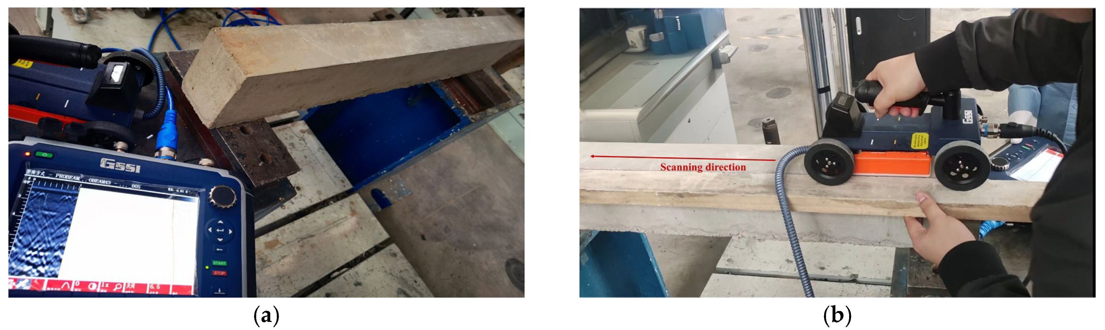
3.3. Laboratory Testing

According to the experimental design specifications, defective concrete beams were manufactured in the laboratory. During the fabrication of the specimens, plastic tape was chosen to control the distance between the defects and the upper surface of the concrete rather than using fine wire. This decision was made because electromagnetic waves are more sensitive to metallic materials, which helps avoid interference from metals and other substances that could affect the test results. Polystyrene foam was employed to represent the small impermeable solid structures found within concrete due to its porous nature. A square wooden box containing slurry-free crushed stone was used to simulate larger, less dense entities. Wood was selected as the exterior material for the impermeable solid because its dielectric constant is similar to that of air.

In another set of experiments, bending tests were conducted on concrete beam H_B0. In the final damaged state, the peak load of the vertically concentrated load force reached 41.27 kN, and the diagonal crack on the surface of the concrete beam reached a 3 mm width. The measurement equipment used in this experiment is the SIR-4000 ground penetrating radar system produced by GSSI company with a 1.6 GHz antenna. The system utilizes high-frequency antennas to provide high detection resolution and can detect structures and defects with smaller scales. Figure 11 shows the precast defects in the concrete beam used in the experiment and the damaged state of the concrete beam after the bending test.

The handheld GPR device used in this study is shown in Figure 12. The two antennas were horizontally offset by dx = 58 mm.

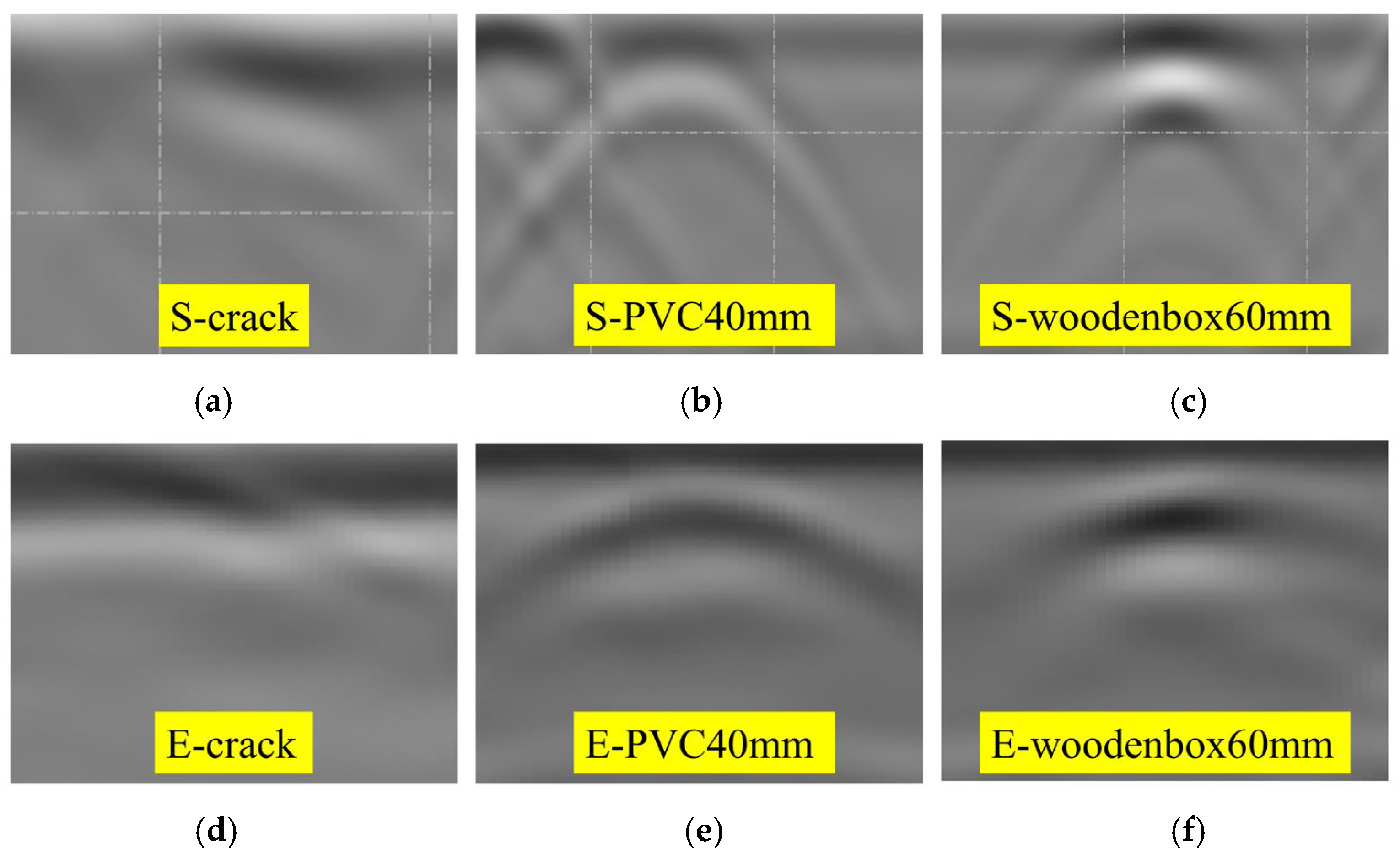
3.4. Results of Experiments and Simulations

Figure 13 shows the comparison between simulated and experimental B-scan results. Cracks, voids, and impermeable solids exhibit significantly different reflection characteristics in the profile. Figure 13a,d shows the reflection of cracks, with longer diagonal cracks appearing more clearly in the cross-section than vertical cracks. A wider crack may result in more pronounced reflections (if the crack is not filled with other media), while a narrower crack may have weaker reflection effects, and reflections may not even appear in the profile. Cracks appear as line reflections on radar profiles, usually narrower and less noticeable than voids.

Figure 13b,e shows the reflection of a PVC pipe with a diameter of 40 mm. PVC pipes usually exhibit strong reflection at the interface under the action of radar waves, forming a downward opening reflection profile. Due to their larger surface area and significant interface reflection effect with concrete, large-diameter PVC pipes usually produce stronger reflection signals, and the boundaries of the reflections are usually clearer and easier to identify.

Figure 13c,f shows the reflection profile of a square wooden box. Non-dense solid defects exhibit higher reflection intensity than cracks and PVC pipes in radar profiles. However, due to their less dense internal structure, irregular scattering and absorption are observed on both sides of the profile line, resulting in faster attenuation of signal intensity.

During the process of processing simulation and experimental signals, A-scan signals were extracted at the vertices of each defect reflection contour and conducted spectral analysis (see Figure 14). In the time domain signal, whether it is a simulated signal or an experimentally measured signal, the reflection of non-dense solids within the 1–2 ns interval has the largest amplitude response, indicating that their internal regions have higher reflectivity, which may be due to their larger dielectric constant or richer internal structure. The 3–4 ns interval is the reflection at the bottom interface of the concrete beam, where the reflection amplitude of the crack is higher than the other two groups; this is because the crack runs through the entire concrete beam. From the spectrum, it can be seen that 1.6 GHz electromagnetic waves have similar propagation characteristics in different concrete beams, and the reflected signals of three different types of defects have the same main frequency. The amplitude value of non-dense solids at the main frequency position is slightly higher than the other two sets of data. Due to the interference of background noise in the experimental data, we can draw the fitting curve of the experimental data and see that with the increase of frequency, both simulation and experimental signals indicate that the reflection amplitude of non-dense solids is significantly higher than that of voids and cracks. This indicates that air has a significant absorption and attenuation effect on the high-frequency components of electromagnetic waves. Meanwhile, there is a good correlation between the intensity of spectral amplitude values and the reflection intensity of different defects displayed in B-scan images.

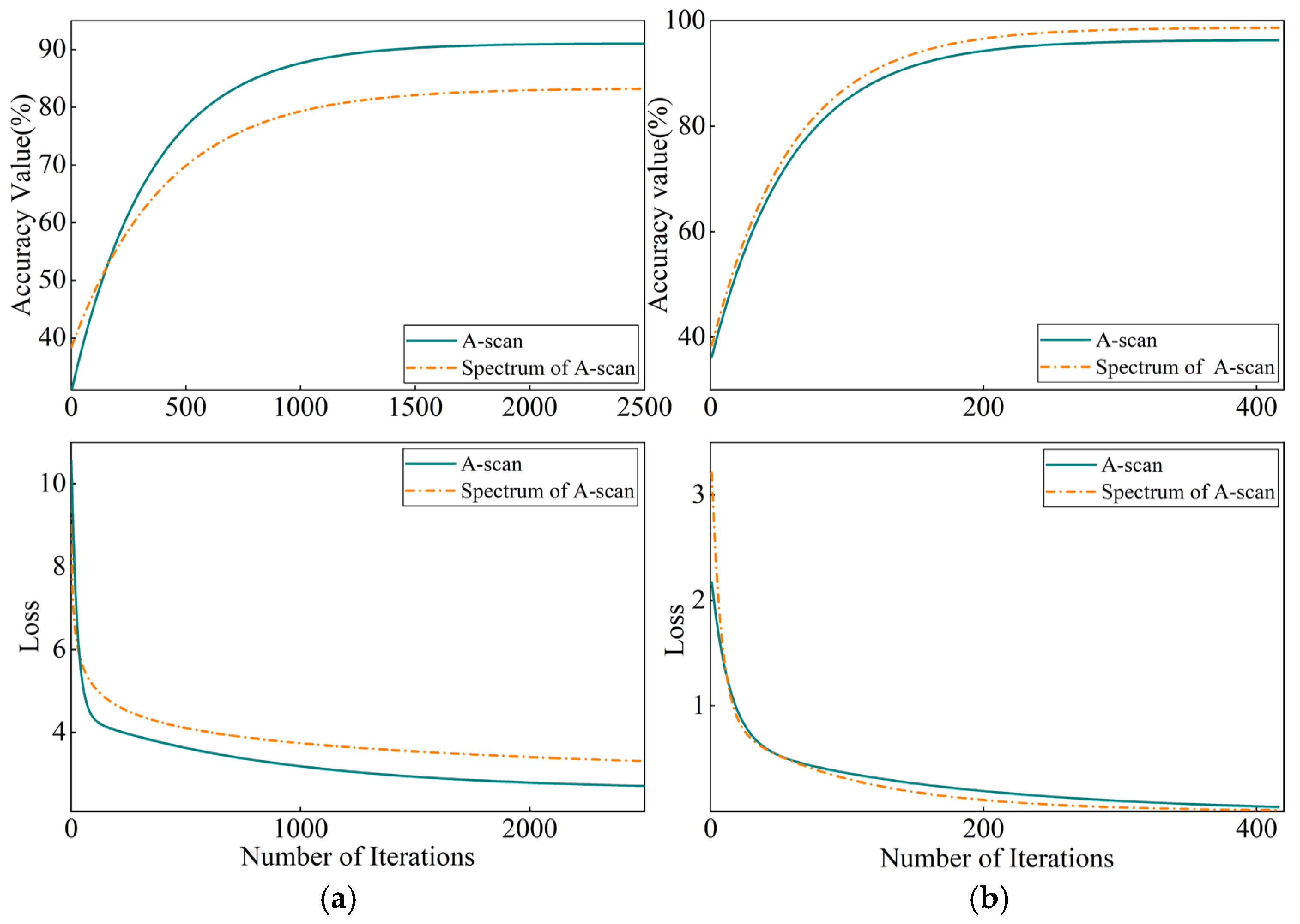
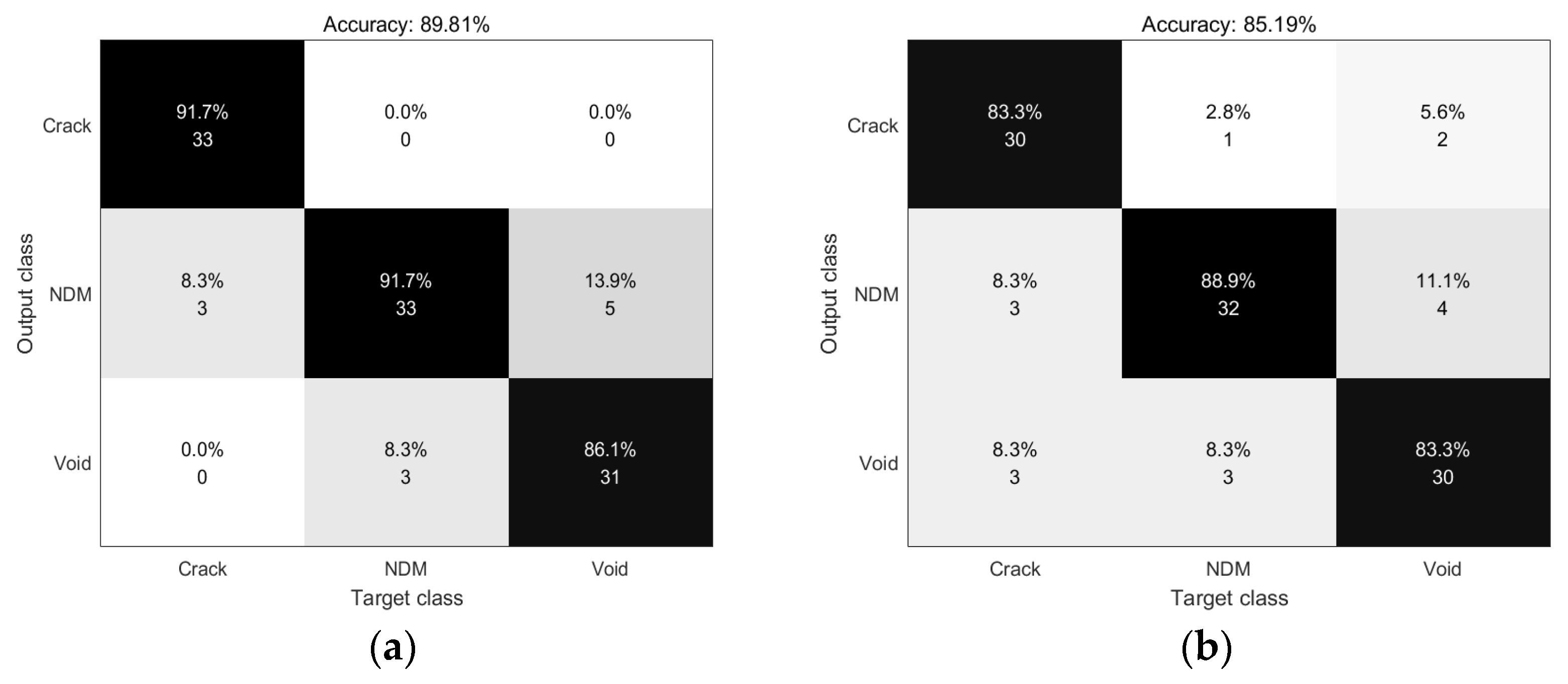
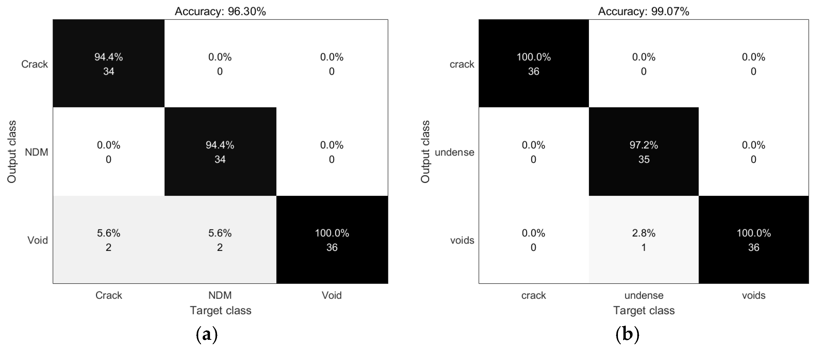
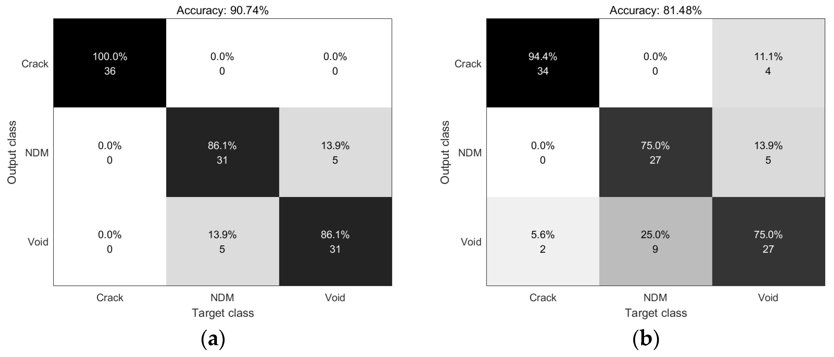
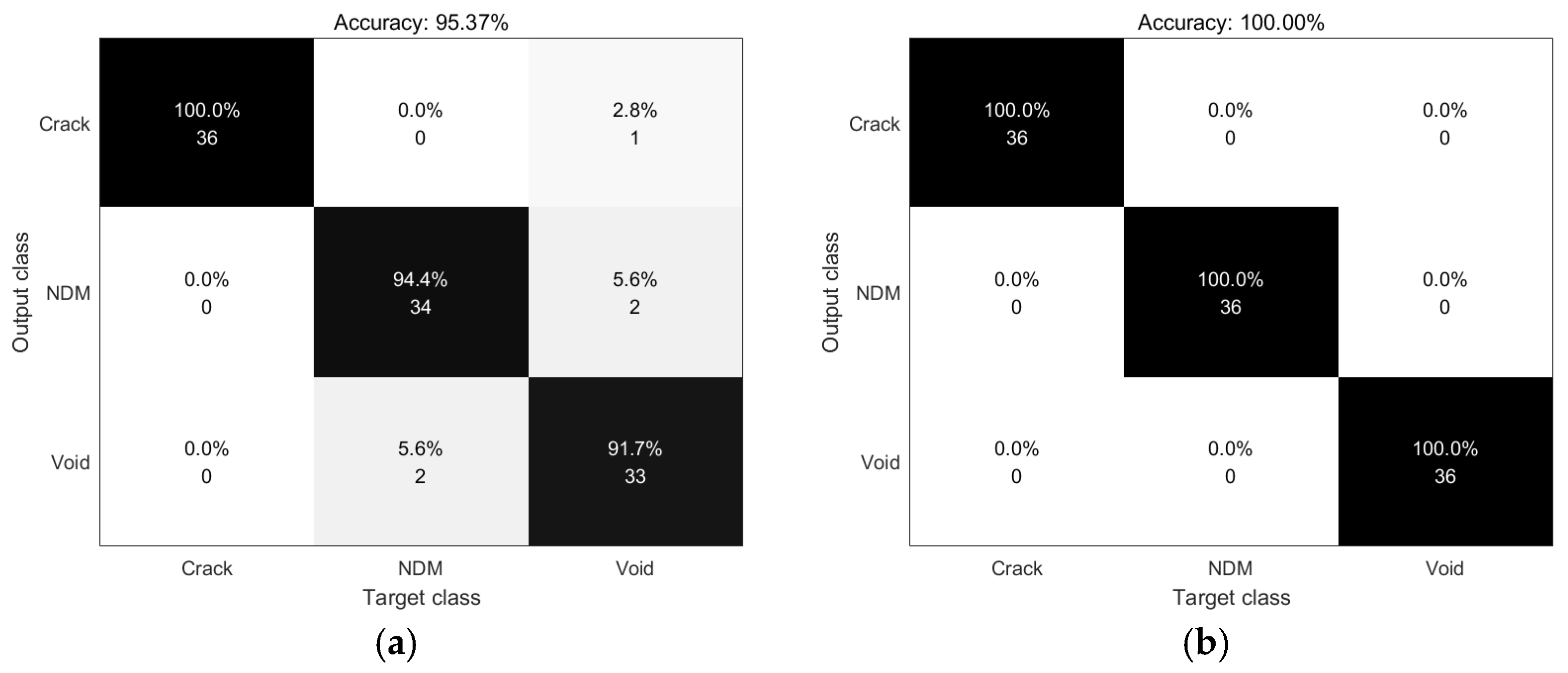
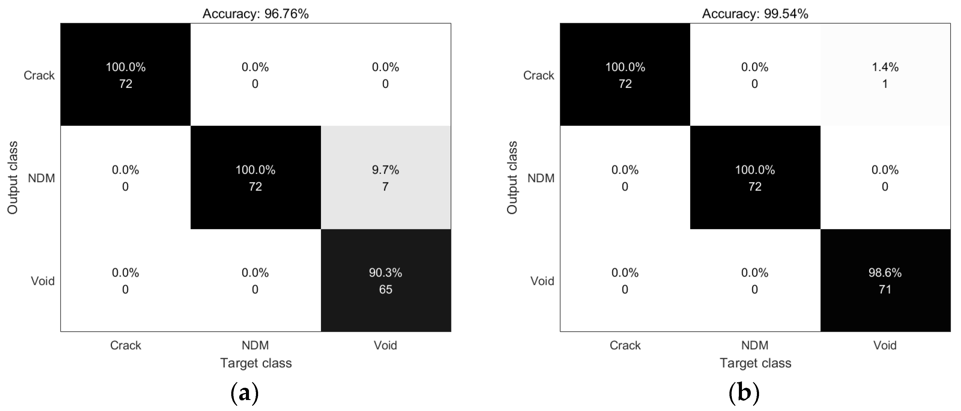
4. Training Process and Results

One hundred twenty experimental and 120 simulated data samples were collected at defect locations of each different concrete beam. The total samples of the experiment and simulation were randomly selected as 70% for training and 30% for validation, with a learning rate of 0.0001 for both datasets. Figure 15 illustrates the fitting curves of validation accuracy and loss over the number of iterations for the CNN model using experimental data in both dimensions. In the one-dimensional CNN training process shown in Figure 15a, compared with frequency domain data, A-scan data exhibits significantly faster convergence speed and lower loss. On the contrary, the two-dimensional CNN training results in Figure 15b show different trends. During the verification process, the accuracy curves of the spectrum and A-scan image almost overlapped. However, the final verification result of the spectrum was slightly higher than that of the A-scan, while its loss was relatively low. Compared with the one-dimensional CNN model, the spectral data achieved better fitting in the two-dimensional CNN model, demonstrating stronger robustness. As the number of iterations increases, spectral data can converge to the optimal state faster.

The classification results in this article are visualized in the form of a confusion matrix, which is an important tool for evaluating the performance of classification models. It displays the relationship between the model’s predicted results and the actual results in a matrix format. The depth of the colors in the blocks of the confusion matrix is typically used to represent the quantity or proportion of predictions for each category; generally, the darker the color, the higher the quantity or ratio represented in that section.

Figure 16 and Figure 17 show the validation results of the confusion matrix obtained after training the numerical simulation data in one-dimensional CNN and two-dimensional CNN, respectively. In the one-dimensional CNN model, the recognition accuracy of different types of defects in the A-scan spectrum is higher than that in the A-scan spectrum. In contrast, the results in the two-dimensional CNN model are exactly the opposite. Overall, the recognition accuracy of the two-dimensional CNN model for different types of defects in the A-scan and A-scan spectrum is significantly higher than that of the one-dimensional CNN model. In the validation results of the one-dimensional CNN model, 8.3% of cracks were identified as non-dense solids, and more than 10% of voids data were identified as non-dense solids. This situation was effectively improved in the validation results of the two-dimensional CNN model.

Figure 18 and Figure 19 show the validation results of the confusion matrix obtained after training the one-dimensional CNN model and the two-dimensional CNN model, respectively. The verification results are very similar to the simulation data, and the recognition accuracy of A-scan data is better than A-scan spectrum data in one-dimensional CNN models, while the recognition accuracy of A-scan spectrum data is higher in two-dimensional CNN models. It is worth mentioning that the validation results of the A-scan spectrum data obtained in the experiment in the one-dimensional CNN model were lower than those of the simulation data, while the validation results of the A-scan spectrum data obtained in the experiment in the two-dimensional CNN model reached 100%. This indicates that compared with one-dimensional data, two-dimensional data can provide richer data information. Compared with time-domain data, frequency-domain data can also provide learning features such as frequency response and frequency band distribution for the two-dimensional CNN model.

In order to improve the generalization ability of the two-dimensional CNN model, simulated data and experimental data are combined for training and classification (see Figure 20). From the results, it can be seen that errors mainly occur in the feature recognition of voids, while the feature classification of cracks and non-dense solids is more accurate.

Figure 21 provides a more intuitive display of the classification and statistical results of experimental and simulated data trained using one-dimensional and two-dimensional CNN models in this study. In the results of the one-dimensional CNN model, the training results of A-scan data are higher than those of spectrum data. In the training results of the two-dimensional CNN model, the overall recognition accuracy is significantly higher than that of the one-dimensional CNN model. At the same time, the results of A-scan spectrum data are higher than those of A-scan data, further verifying the learning ability of the two-dimensional CNN model for spatial and local features of complex data.

5. Conclusions and Discussion

Aiming at different types of defects in small-scale reinforced concrete members, this paper proposes A nondestructive testing method combining A-scan data and A-scan spectrum data in GPR signal with CNN. Through the processing and analysis of the experimental data and the simulated electromagnetic wave response data of reinforced concrete beams with complex three-dimensional media, the results show that the one-dimensional CNN model performs better in extracting A-scan data features than A-scan spectrum data. Compared with the one-dimensional CNN model, the two-dimensional CNN architecture AlexNet has the advantages of deeper network structure, more parameters, introduces ReLU activation function, etc. The verification results of experimental and simulated data also show that AlexNet has higher accuracy and reliability and has more advantages in processing complex data. It is also proved that the spectrum data with more abundant information can be used as the input data of the two-dimensional CNN model to train and detect the damage of concrete structures.

However, this non-destructive testing method also has certain limitations. Firstly, the location of A-scan data extraction needs to be as close as possible to the vertex of the reflection profile line. Otherwise, it cannot reflect the signal characteristics of a certain type of damage. Secondly, the number of data samples used for CNN training should not be too small, as too little training data will affect the generalization ability of the CNN model. In addition, there are significant challenges in the application of GPR methods for small-scale crack damage in concrete structures. How to use GPR combined with CNN methods to solve such problems is also something that needs to be attempted in the future of this study.

References

1. Worden, K.; Farrar, C.R.; Manson, G.; Park, G. The fundamental axioms of structural health monitoring. Proc. R. Soc. A Math. Phys. Eng. Sci. 2007, 463, 1639–1664. [Google Scholar] [CrossRef]
2. Durmus, A.; Ozturk, H.T.; Durmus, A. A reliable approach for determining concrete strength in structures by using cores. Comput. Concr. 2013, 11, 463–473. [Google Scholar] [CrossRef]
3. Patil, S.; Banerjee, S.; Tallur, S. Smart structural health monitoring (SHM) system for on-board localization of defects in pipes using torsional ultrasonic guided waves. Sci. Rep. 2024, 14, 24455. [Google Scholar] [CrossRef]
4. Liu, Z.; Gu, X.; Wu, C.; Ren, H.; Zhou, Z.; Tang, S. Studies on the validity of strain sensors for pavement monitoring: A case study for a fiber Bragg grating sensor and resistive sensor. Constr. Build. Mater. 2022, 321, 126085. [Google Scholar] [CrossRef]
5. Benedetto, A.; Tosti, F.; Bianchini Ciampoli, L.; D’Amico, F. An overview of ground-penetrating radar signal processing techniques for road inspections. Signal Process 2017, 132, 201–209. [Google Scholar] [CrossRef]
6. Farahani, R.V.; Penumadu, D. Damage identification of a full-scale five-girder bridge using time-series analysis of vibration data. Eng. Struct. 2016, 115, 129–139. [Google Scholar] [CrossRef]
7. Tosti, F.; Ferrante, C. Using Ground Penetrating Radar Methods to Investigate Reinforced Concrete Structures. Surv. Geophys. 2019, 41, 485–530. [Google Scholar] [CrossRef]
8. Dinh, K.; Gucunski, N. Factors affecting the detectability of concrete delamination in GPR images. Constr. Build. Mater. 2021, 274, 121837. [Google Scholar] [CrossRef]
9. Liu, X.; Hao, P.; Wang, A.; Zhang, L.; Gu, B.; Lu, X. Non-destructive detection of highway hidden layer defects using a ground-penetrating radar and adaptive particle swarm support vector machine. Peerj Comput. Sci. 2021, 7, e417. [Google Scholar] [CrossRef]
10. Gucunski, N.; Kim, J.; Duong, T.H. Understanding depth-amplitude effects in assessment of GPR data from concrete bridge decks. NdtE Int. 2016, 83, 48–58. [Google Scholar] [CrossRef]
11. Hong, S.; Mo, G.; Song, S.; Li, D.; Huang, Z.; Hou, D.; Chen, H.; Mao, X.; Lou, X.; Dong, B. Research on reinforcement corrosion detection method based on the numerical simulation of ground-penetrating radar. J. Build. Eng. 2024, 85, 108760. [Google Scholar] [CrossRef]
12. Tesic, K.; Baricevic, A.; Serdar, M.; Gucunski, N. Characterization of ground penetrating radar signal during simulated corrosion of concrete reinforcement. Autom. Constr. 2022, 143, 104548. [Google Scholar] [CrossRef]
13. Zhang, W.; Sun, K.; Lei, C.; Zhang, Y.; Li, H.; Spencer, B.F. Fuzzy Analytic Hierarchy Process Synthetic Evaluation Models for the Health Monitoring of Shield Tunnels. Comput.-Aided Civ. Inf. 2014, 29, 676–688. [Google Scholar] [CrossRef]
14. Krizhevsky, A.; Sutskever, I.; Hinton, G.E. ImageNet Classification with Deep Convolutional Neural Networks. Commun. ACM 2017, 60, 84–90. [Google Scholar] [CrossRef]
15. Bao, Y.; Tang, Z.; Li, H.; Zhang, Y. Computer vision and deep learning–based data anomaly detection method for structural health monitoring. Struct. Health Monit. 2018, 18, 401–421. [Google Scholar] [CrossRef]
16. Travassos, X.L.; Avila, S.L.; Ida, N. Artificial Neural Networks and Machine Learning techniques applied to Ground Penetrating Radar: A review. Appl. Comput. Inf. 2020, 17, 296–308. [Google Scholar] [CrossRef]
17. Abdeljaber, O.; Avci, O.; Kiranyaz, M.S.; Boashash, B.; Sodano, H.; Inman, D.J. 1-D CNNs for structural damage detection: Verification on a structural health monitoring benchmark data. Neurocomputing 2018, 275, 1308–1317. [Google Scholar] [CrossRef]
18. Xue, Y.; Li, Y. A Fast Detection Method via Region-Based Fully Convolutional Neural Networks for Shield Tunnel Lining Defects. Comput.-Aided Civ. Inf. 2018, 33, 638–654. [Google Scholar] [CrossRef]
19. Zhou, Z.; Zhang, J.; Gong, C. Automatic detection method of tunnel lining multi-defects via an enhanced You Only Look Once network. Comput.-Aided Civ. Inf. 2022, 37, 762–780. [Google Scholar] [CrossRef]
20. Guo, S.; Yang, T.; Gao, W.; Zhang, C. A Novel Fault Diagnosis Method for Rotating Machinery Based on a Convolutional Neural Network. Sensors 2018, 18, 1429. [Google Scholar] [CrossRef]
21. Zhang, Y.; Miyamori, Y.; Mikami, S.; Saito, T. Vibration-based structural state identification by a 1-dimensional convolutional neural network. Comput.-Aided Civ. Inf. 2019, 34, 822–839. [Google Scholar] [CrossRef]
22. Abdeljaber, O.; Avci, O.; Kiranyaz, S.; Gabbouj, M.; Inman, D.J. Real-time vibration-based structural damage detection using one-dimensional convolutional neural networks. J. Sound Vib. 2017, 388, 154–170. [Google Scholar] [CrossRef]
23. Mao, G.; Zhang, Z.; Qiao, B.; Li, Y. Fusion Domain-Adaptation CNN Driven by Images and Vibration Signals for Fault Diagnosis of Gearbox Cross-Working Conditions. Entropy 2022, 24, 119. [Google Scholar] [CrossRef]
24. Kim, N.; Kim, S.; An, Y.-K.; Lee, J.-J. A novel 3D GPR image arrangement for deep learning-based underground object classification. Int. J. Pavement. Eng. 2019, 22, 740–751. [Google Scholar] [CrossRef]
25. Liu, W.; Luo, R.; Xiao, M.; Chen, Y. Intelligent detection of hidden distresses in asphalt pavement based on GPR and deep learning algorithm. Constr. Build. Mater. 2024, 416, 135089. [Google Scholar] [CrossRef]
26. Zhang, J.; Yang, X.; Li, W.; Zhang, S.; Jia, Y. Automatic detection of moisture damages in asphalt pavements from GPR data with deep CNN and IRS method. Autom. Constr. 2020, 113, 103119. [Google Scholar] [CrossRef]
27. Gao, J.; Yuan, D.; Tong, Z.; Yang, J.; Yu, D. Autonomous pavement distress detection using ground penetrating radar and region-based deep learning. Measurement 2020, 164, 108077. [Google Scholar] [CrossRef]
28. Jazayeri, S.; Saghafi, A.; Esmaeili, S.; Tsokos, C.P. Automatic object detection using dynamic time warping on ground penetrating radar signals. Expert. Syst. Appl. 2019, 122, 102–107. [Google Scholar] [CrossRef]
29. Xu, J.; Zhang, J.; Sun, W. Recognition of the Typical Distress in Concrete Pavement Based on GPR and one-dimensional. Remote Sens. 2021, 13, 2375. [Google Scholar] [CrossRef]
30. Li, X.; Liu, H.; Zhou, F.; Chen, Z.; Giannakis, I.; Slob, E. Deep learning–based nondestructive evaluation of reinforcement bars using ground-penetrating radar and electromagnetic induction data. Comput.-Aided Civ. Infrastruct. Eng. 2022, 37, 1834–1853. [Google Scholar] [CrossRef]
31. He, R.; Lu, N. Unveiling the dielectric property change of concrete during hardening process by ground penetrating radar with the antenna frequency of 1.6 GHz and 2.6 GHz. Cem. Concr. Comp. 2023, 144, 105279. [Google Scholar] [CrossRef]
32. Zhong, Y.; Wang, Y.; Zhang, B. Research on correlation between dielectric properties and compressive strength of concrete based on aggregate particle size. J. Build. Eng. 2024, 97, 110844. [Google Scholar] [CrossRef]
33. Lachowicz, J.; Rucka, M. A novel heterogeneous model of concrete for numerical modelling of ground penetrating radar. Constr. Build. Mater. 2019, 227, 116703. [Google Scholar] [CrossRef]
34. Warren, C.; Giannopoulos, A.; Giannakis, I. gprMax: Open source software to simulate electromagnetic wave propagation for Ground Penetrating Radar. Comput. Phys. Commun. 2016, 209, 163–170. [Google Scholar] [CrossRef]
35. Warren, C.; Giannopoulos, A.; Gray, A.; Giannakis, I.; Patterson, A.; Wetter, L.; Hamrah, A. A CUDA-based GPU engine for gprMax: Open source FDTD electromagnetic simulation software. Comput. Phys. Commun. 2019, 237, 208–218. [Google Scholar] [CrossRef]
Figure 1. Diagram of the GPR detection concrete distress principle.
Applsci 15 01882 g001
Figure 2. Process of the one-dimensional convolution layer.
Applsci 15 01882 g002
Figure 3. Process of the two-dimensional convolution layer.
Applsci 15 01882 g003
Figure 4. Process of the pooling layer.
Applsci 15 01882 g004
Figure 5. The diagram is one-dimensional.
Applsci 15 01882 g005
Figure 6. The diagram is two-dimensional.
Applsci 15 01882 g006
Figure 7. (a) H_B0: reinforced concrete beam; (b) H_BF1: 40 mm diameter PVC pipe and 60 mm side length of non-confined solid; (c) H_BF2: 25 mm diameter PVC pipe and 30 mm side length plastic foam.
Applsci 15 01882 g007
Figure 8. A heterogeneous numerical model of concrete.
Applsci 15 01882 g008
Figure 9. Models of concrete beams with defects: (a) H_B0; (b) H_BF1; (c) H_BF2.
Applsci 15 01882 g009
Figure 10. Concrete surface line tracks.
Applsci 15 01882 g010
Figure 11. The setting of prefabricated defects in concrete beams: (a) non-dense material, void, and (b) cracks generated during the experiment.
Applsci 15 01882 g011
Figure 12. (a) GSSI GPR equipment and (b) measurement process.
Applsci 15 01882 g012
Figure 13. Radar profile features of different defects (Figure (ac) are simulation results, while Figure (df) are experiment results).
Applsci 15 01882 g013
Figure 14. Comparison of (a) simulated A-scan and (b) spectrum of simulated A-scan for three different defect types; (c) experimental A-scan and (d) spectrum of experimental A-scan for three different defect types.
Applsci 15 01882 g014
Figure 15. The fitting curves of the training process of two kinds of convolutional networks for (a) the one-dimensional CNN and (b) the two-dimensional CNN.
Applsci 15 01882 g015
Figure 16. Classification results of one-dimensional CNN model for simulated data for (a) the A-scan and (b) the spectrum of the A-scan.
Applsci 15 01882 g016
Figure 17. Classification results of two-dimensional CNN model for simulated data for (a) the A-scan and (b) the spectrum of the A-scan.
Applsci 15 01882 g017
Figure 18. Classification results of one-dimensional CNN model for experimental data for (a) the A-scan and (b) the spectrum of the A-scan.
Applsci 15 01882 g018
Figure 19. Classification results of two-dimensional CNN model for experimental data for (a) the A-scan and (b) the spectrum of the A-scan.
Applsci 15 01882 g019
Figure 20. Classification results of two-dimensional CNN model for merged data for (a) the A-scan and (b) the spectrum of the A-scan.
Applsci 15 01882 g020
Figure 21. Accuracy values for training on experimental and simulated data using (a) the one-dimensional CNN model and (b) the two-dimensional CNN model.
Applsci 15 01882 g021