

IoT-Driven Resilience Monitoring: Case Study of a Cyber-Physical System

 , ,
, ,  , , and
Abstract
:1. Introduction
- The development and validation of a comprehensive method for real-time resilience monitoring of IoT-integrated CI.
- The implementation and testing of different data-driven algorithms tailored to R-KPIs, informed by observed system behavior.
- The construction and operation of a practical cyber-physical testbed for empirical resilience assessment using a Digital Twin-integrated smart PV system.
2. Research Landscape
Next-Gen Energy Systems Resilience
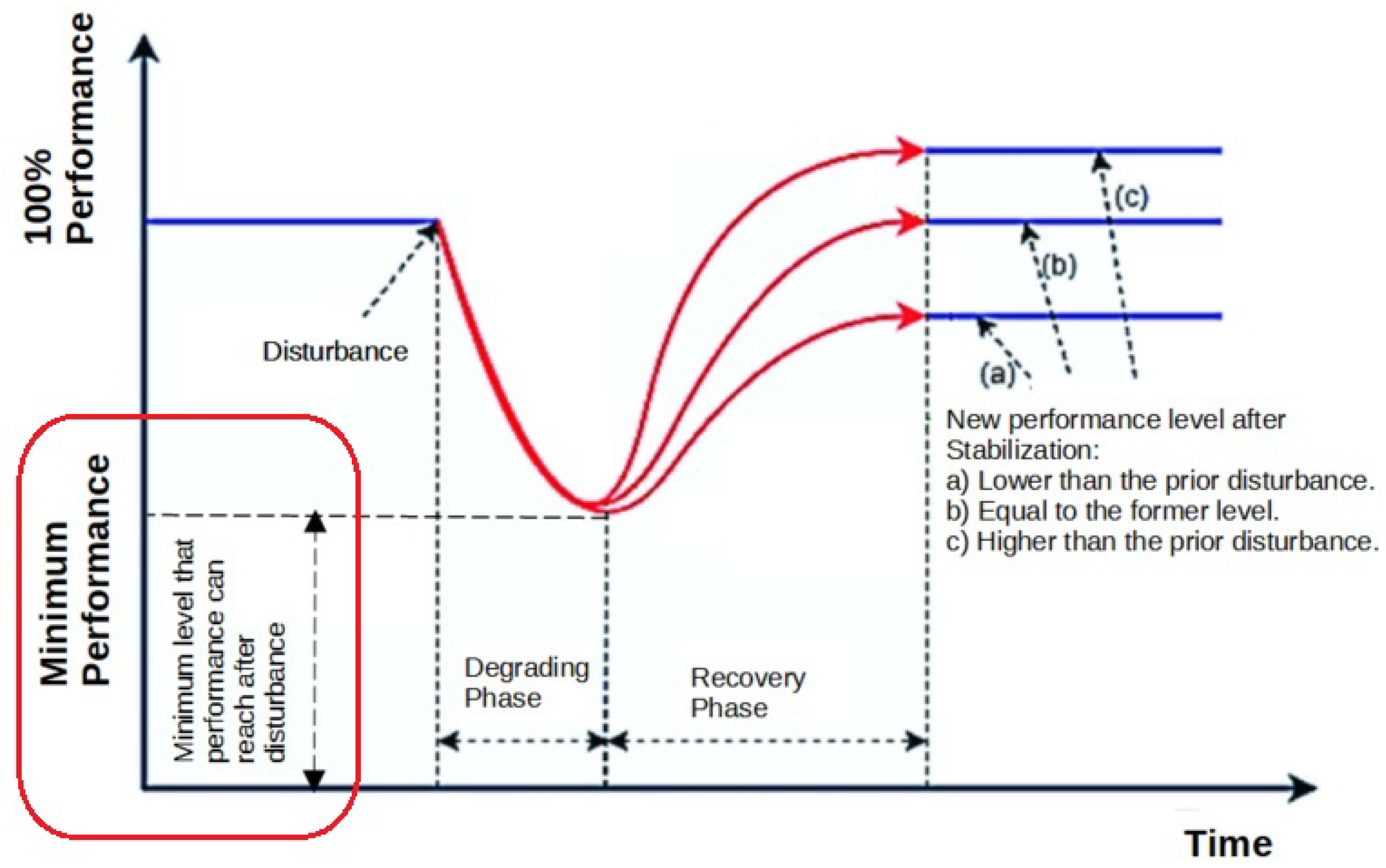
3. Theoretical Foundation of Resilience Curve and Its KPIs in This Domain
3.1. Resilience Curve and Selected R-KPIs
3.1.1. Recovery Time
3.1.2. Minimum Performance Level
3.1.3. Functionality Loss
4. Implemented Statistical and AI Methods
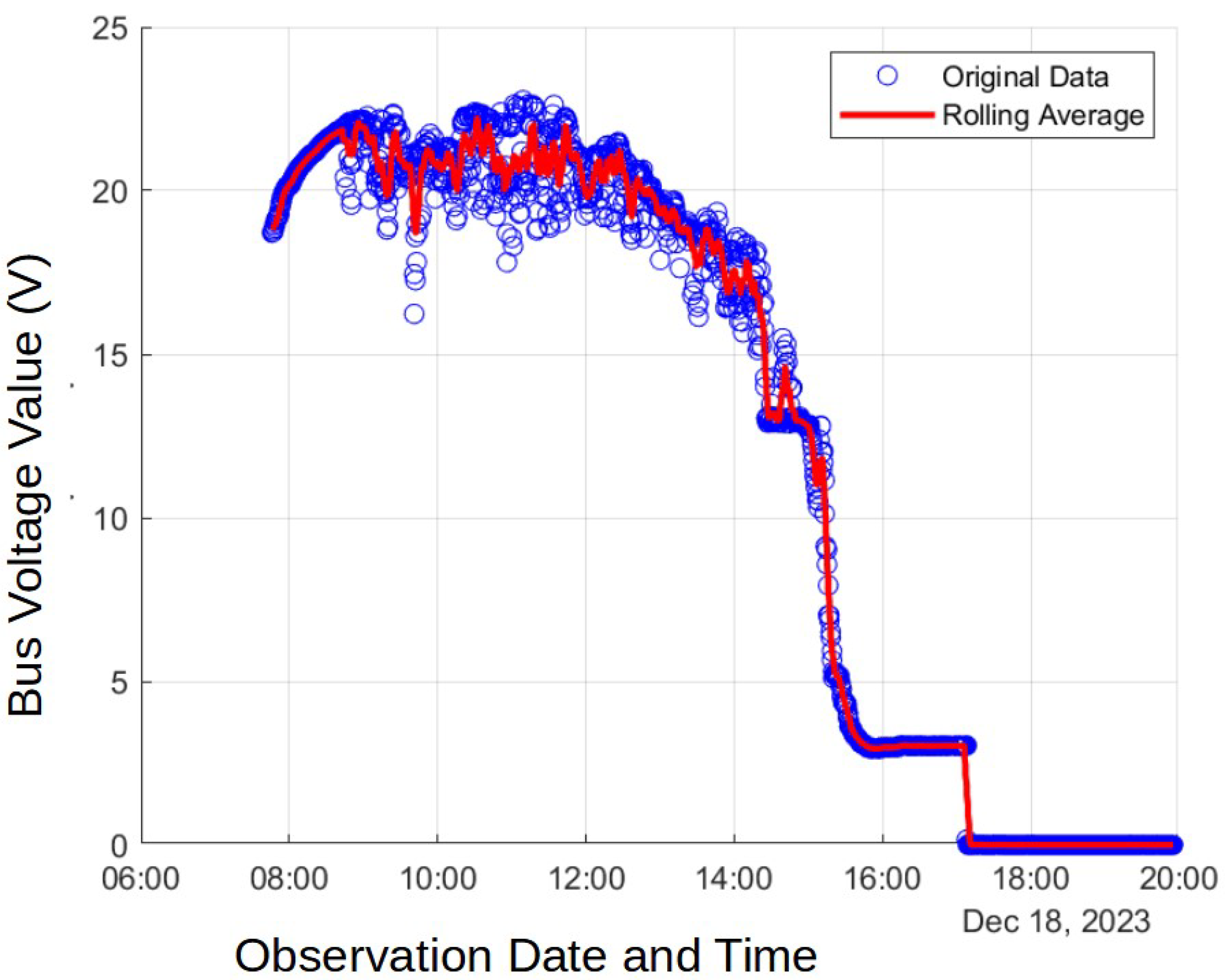
4.1. Moving Average
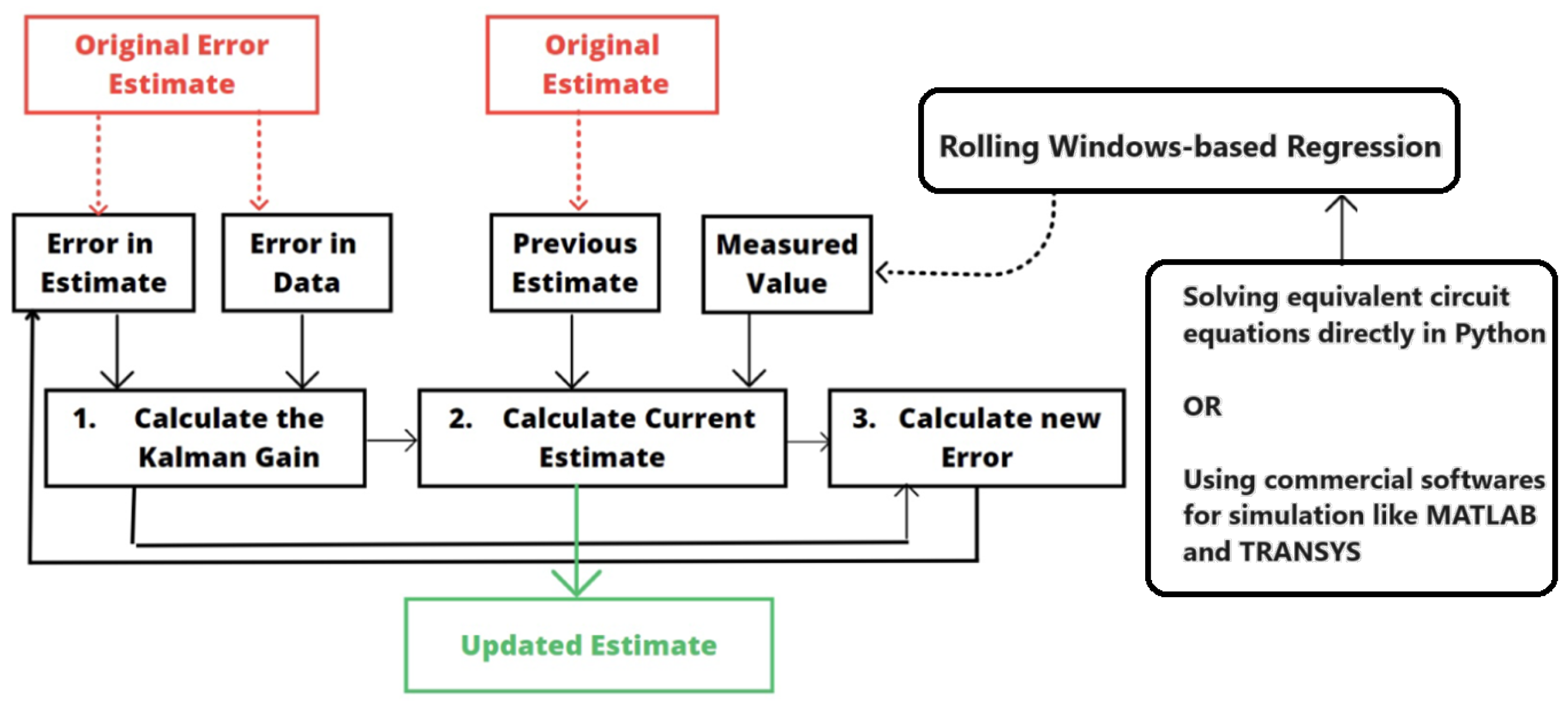
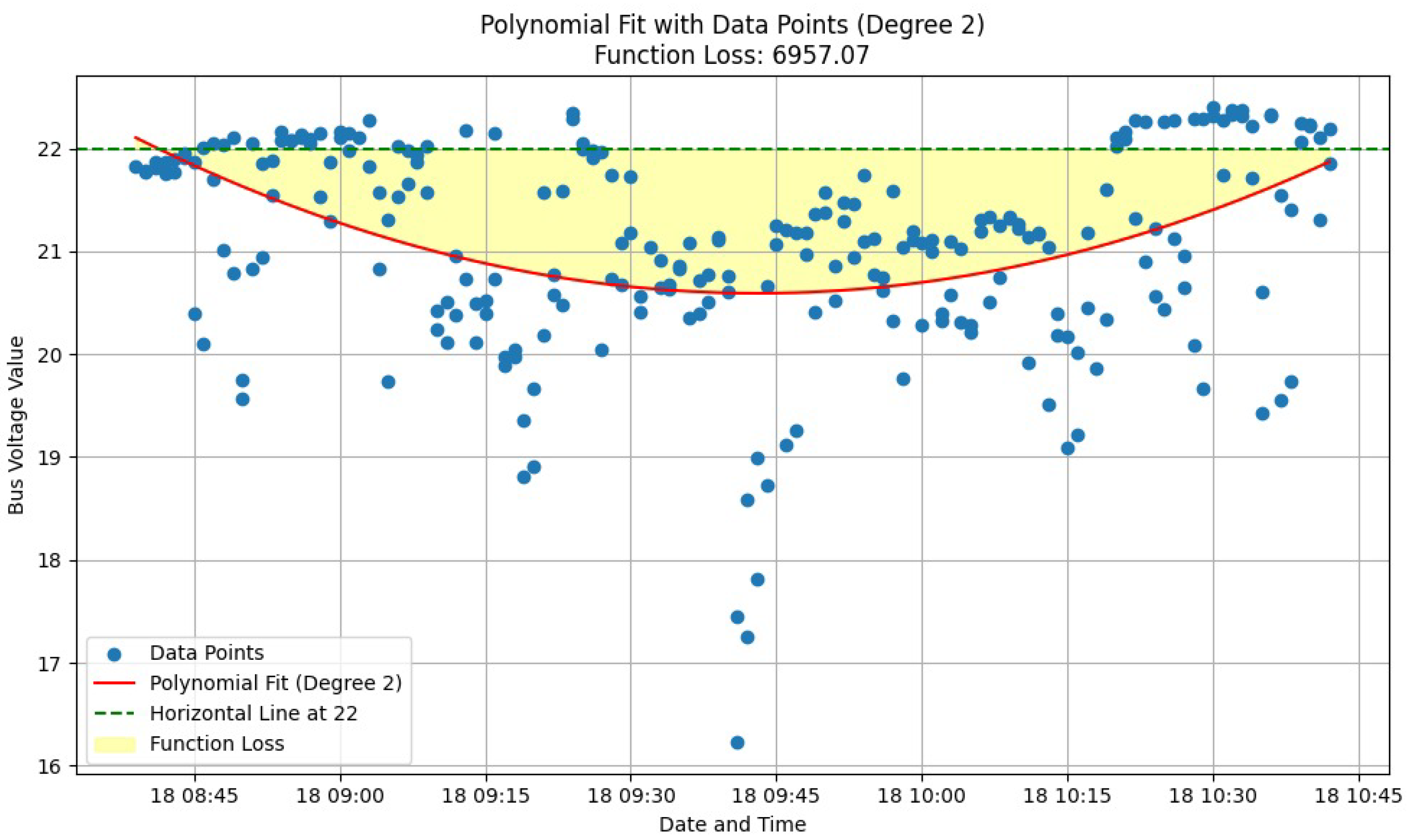
4.2. Least Squares Regression
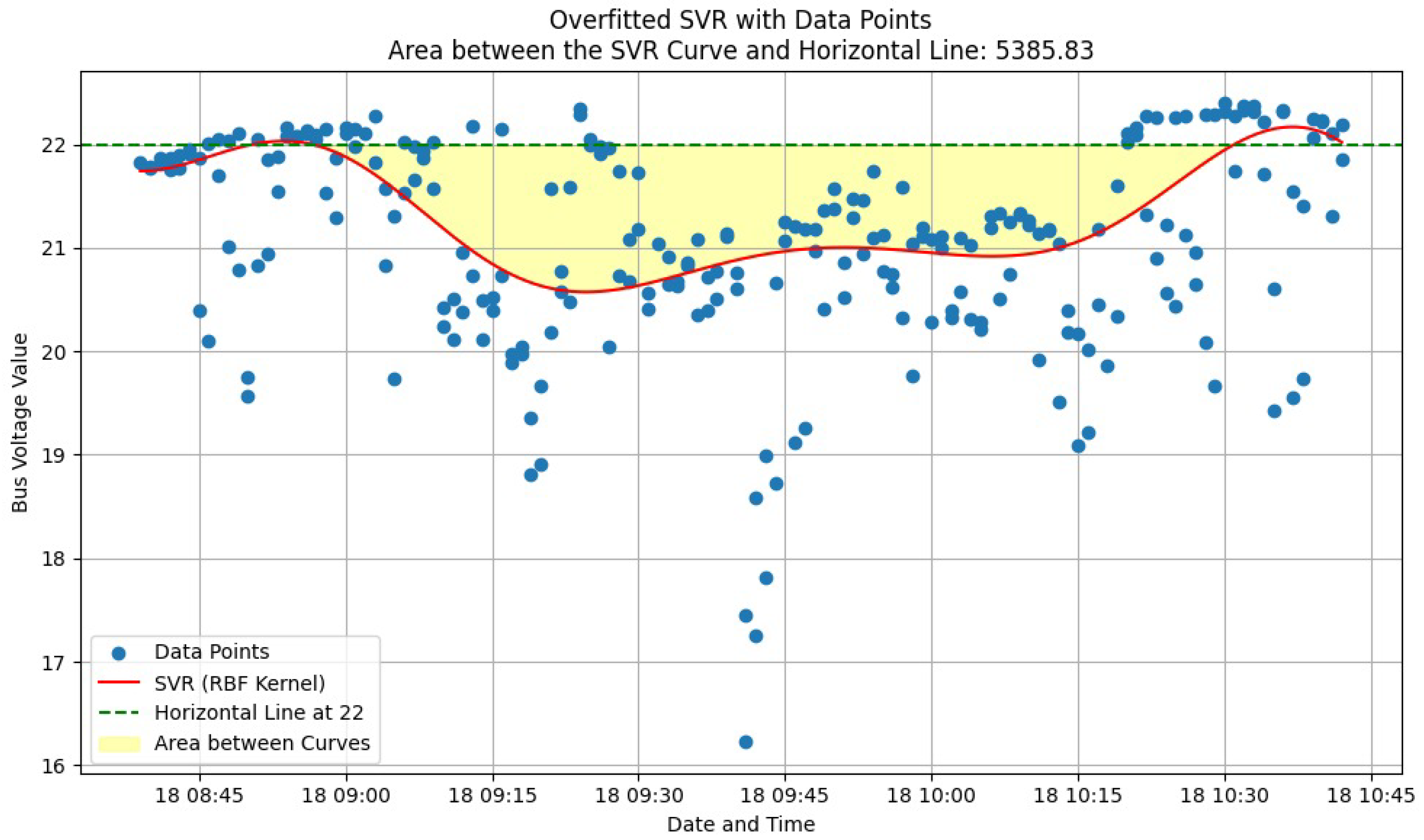
4.3. Support Vector Regression (SVR) Model with a Radial Basis Function (RBF) Kernel
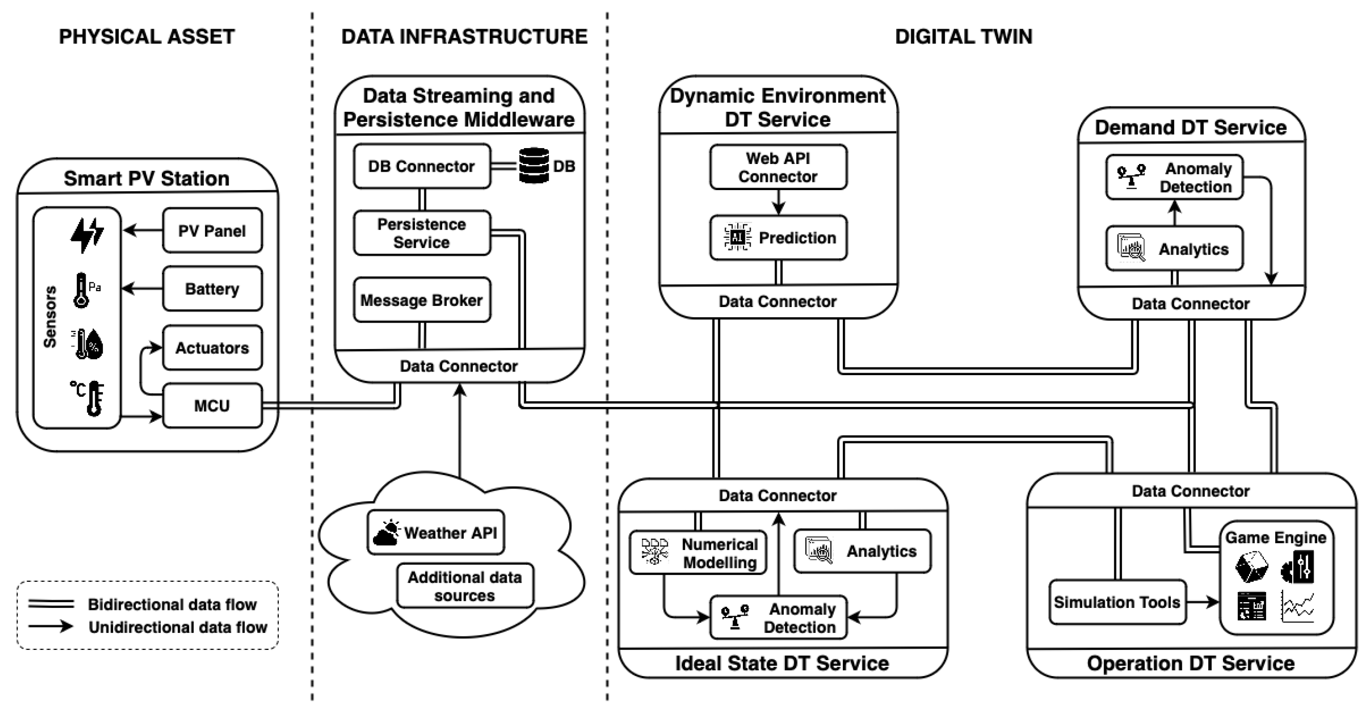
5. Cyber-Physical System
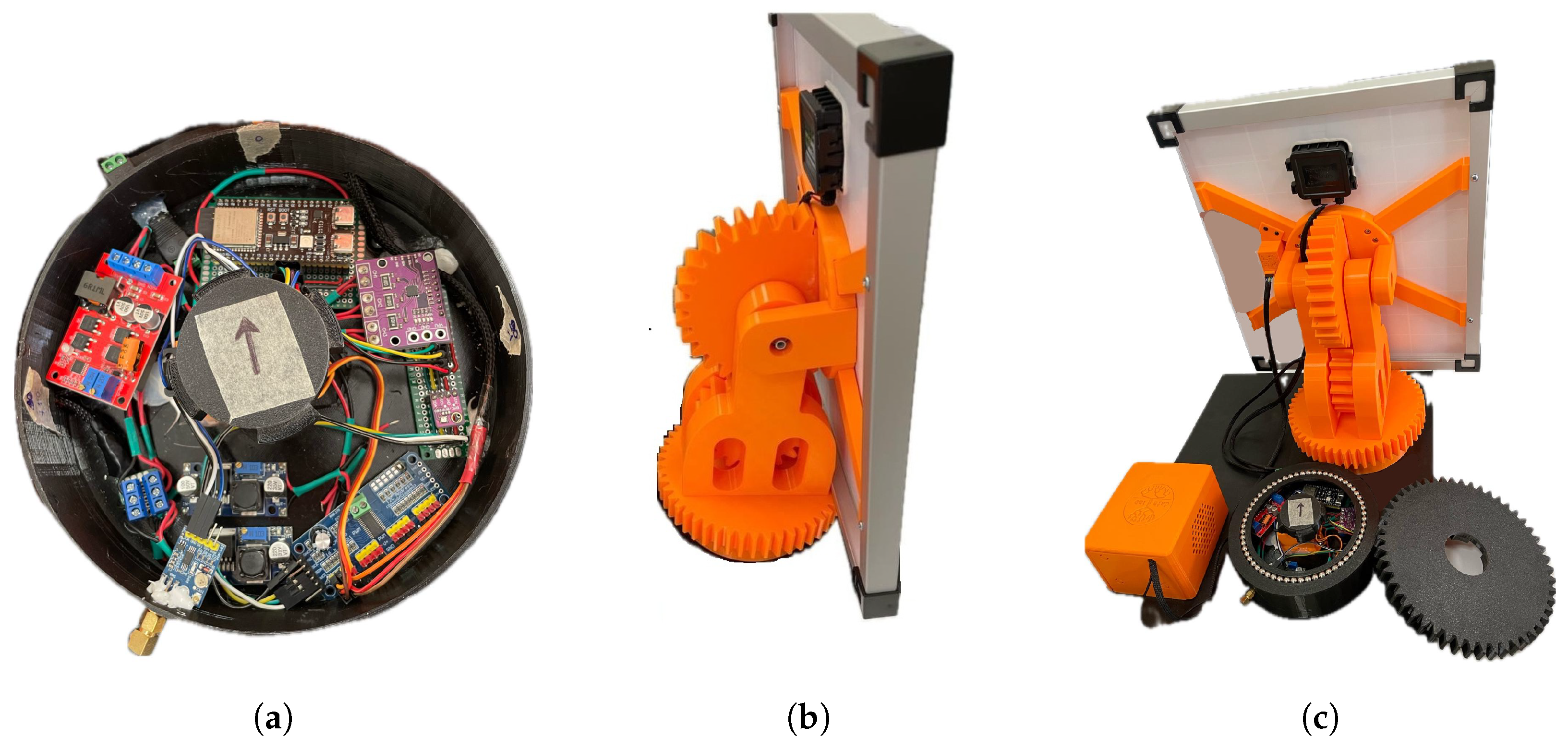
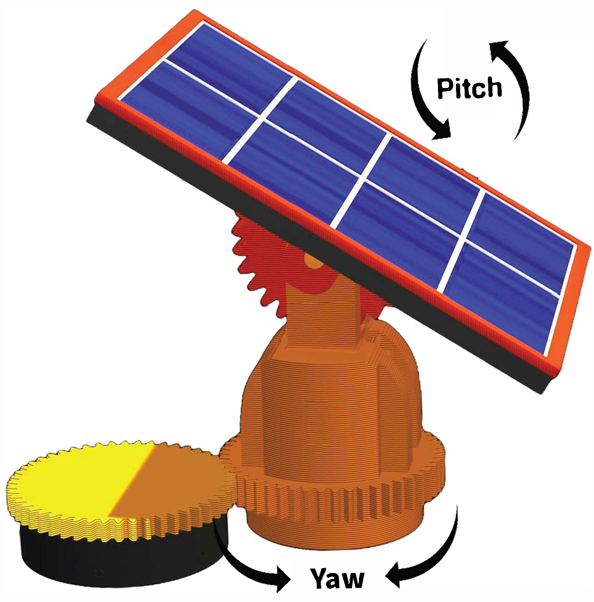
5.1. Physical Asset: Smart PhotoVoltaic Station
5.1.1. PV Panel
5.1.2. Sensors and Actuators
5.1.3. Service Modules
5.2. Data Infrastructure: Data Streaming and Persistence Middleware
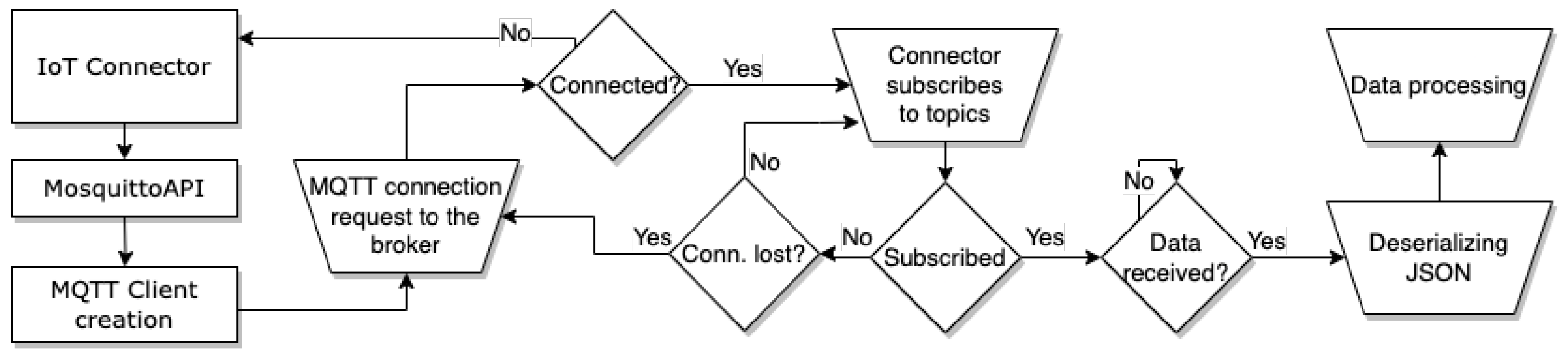
5.2.1. Data Streaming
5.2.2. Data Persistence
5.3. Energy Digital Twin: Virtual World Interactive Model
5.3.1. Dynamic Environment Service
5.3.2. Operation Service
5.3.3. Ideal State Service
5.3.4. Demand Service
5.3.5. Service Deployment
6. Case Study
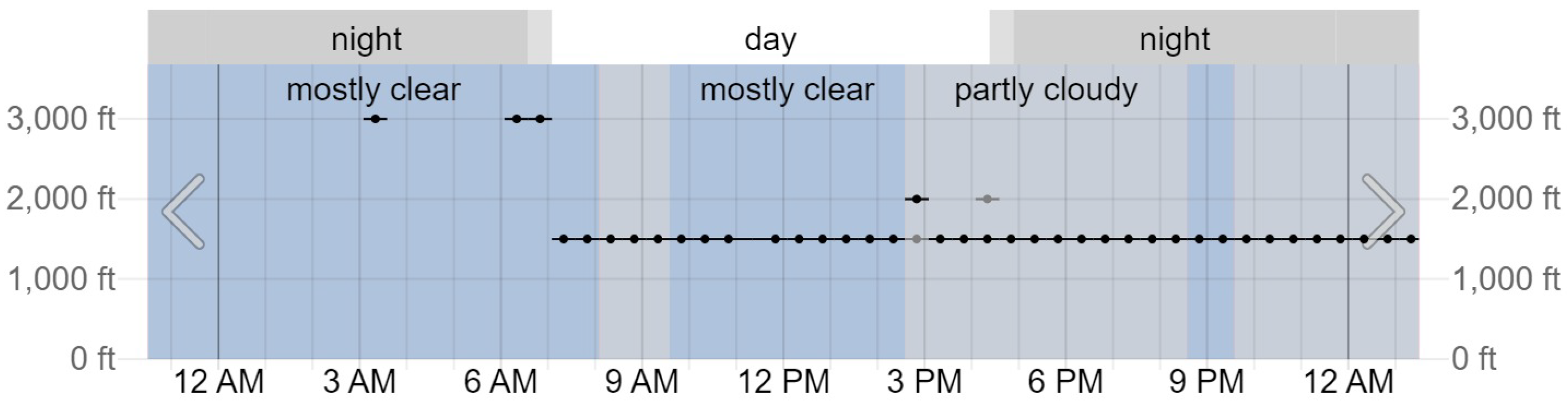
6.1. Test Condition
- Temperature: Ranged from 11 °C to 14 °C.
- Atmospheric Pressure: Maintained at around 1030 to 1034 hPa.
- Wind: Predominantly from the NW direction, with speeds varying from 17 to 31 km/h.
- Visibility: ≥10 km throughout the day.
- Cloud Cover: Mostly clear and partly cloudy, with occasional cloud layers at 450 to 600 m.
- Dew Point: Varied between 9 °C and 11 °C.
6.2. Test Procedure
6.3. Disturbance Scenario
6.4. Testbed Functionality Validation
6.5. Resilience Quantification and Synthesis Results
7. Limitations, Challenges, and Future Study
8. Conclusions
Author Contributions
Funding
Institutional Review Board Statement
Informed Consent Statement
Data Availability Statement
Conflicts of Interest
References
- Radanliev, P.; De Roure, D.; Van Kleek, M.; Santos, O.; Ani, U. Artificial intelligence in cyber physical systems. AI Soc. 2020, 36, 783–796. [Google Scholar] [CrossRef] [PubMed]
- Batista e Silva, F.; Forzieri, G.; Marin Herrera, M.A.; Bianchi, A.; Lavalle, C.; Feyen, L. HARCI-EU, a harmonized gridded dataset of critical infrastructures in Europe for large-scale risk assessments. Sci. Data 2019, 6, 126. [Google Scholar] [CrossRef] [PubMed]
- Cantelmi, R.; Di Gravio, G.; Patriarca, R. Reviewing qualitative research approaches in the context of critical infrastructure resilience. Environ. Syst. Decis. 2021, 41, 341–376. [Google Scholar] [CrossRef] [PubMed]
- Akakura, Y.; Sasaki, T.; Ono, K.; Watanabe, T. An Assessment of the Impacts on the International Container Transport and the World Economy Resulting from the 2014/15 U.S. West Coast Port Disruption. J. Integr. Disaster Risk Manag. 2018, 8, 1–21. [Google Scholar] [CrossRef]
- Gallarno, G.; Muniz, J.; Parnell, G.S.; Pohl, E.A.; Wu, J. Development and assessment of a resilient telecoms system. J. Def. Model. Simul. Appl. Methodol. Technol. 2023, 21, 405–420. [Google Scholar] [CrossRef]
- Koks, E.; Pant, R.; Thacker, S.; Hall, J.W. Understanding Business Disruption and Economic Losses Due to Electricity Failures and Flooding. Int. J. Disaster Risk Sci. 2019, 10, 421–438. [Google Scholar] [CrossRef]
- Avordeh, T.K.; Salifu, A.; Quaidoo, C.; Opare-Boateng, R. Impact of power outages: Unveiling their influence on micro, small, and medium-sized enterprises and poverty in Sub-Saharan Africa - An in-depth literature review. Heliyon 2024, 10, e33782. [Google Scholar] [CrossRef]
- Zhu, Q.; Başar, T. Disentangling Resilience From Robustness: Contextual Dualism, Interactionism, and Game-Theoretic Paradigms. IEEE Control. Syst. Mag. 2024, 44, 95–103. [Google Scholar] [CrossRef]
- Xu, L.; Guo, Q.; Sheng, Y.; Muyeen, S.; Sun, H. On the resilience of modern power systems: A comprehensive review from the cyber-physical perspective. Renew. Sustain. Energy Rev. 2021, 152, 111642. [Google Scholar] [CrossRef]
- Kwasinski, A. Modeling of Cyber-Physical Intra-Dependencies in Electric Power Grids and Their Effect on Resilience. In Proceedings of the 2020 8th Workshop on Modeling and Simulation of Cyber-Physical Energy Systems, Sydney, Australia, 21 April 2020; pp. 1–6. [Google Scholar] [CrossRef]
- Urlainis, A.; Ornai, D.; Levy, R.; Vilnay, O.; Shohet, I.M. Loss and damage assessment in critical infrastructures due to extreme events. Saf. Sci. 2022, 147, 105587. [Google Scholar] [CrossRef]
- Loveček, T.; Straková, L.; Kampová, K. Modeling and Simulation as Tools to Increase the Protection of Critical Infrastructure and the Sustainability of the Provision of Essential Needs of Citizens. Sustainability 2021, 13, 5898. [Google Scholar] [CrossRef]
- Carrington, N.K.; Ma, S.; Dobson, I.; Wang, Z. Extracting Resilience Statistics from Utility Data in Distribution Grids. In Proceedings of the 2020 IEEE Power & Energy Society General Meeting (PESGM), Montreal, QC, Canada, 2–6 August 2020; pp. 1–5. [Google Scholar] [CrossRef]
- Fuggini, C.; Bolletta, F. Identification of indicators, metrics and level of service for the resilience of transport critical infrastructure. Int. J. Sustain. Mater. Struct. Syst. 2020, 4, 330. [Google Scholar] [CrossRef]
- Achillopoulou, D.V.; Mitoulis, S.A.; Argyroudis, S.A.; Wang, Y. Monitoring of transport infrastructure exposed to multiple hazards: A roadmap for building resilience. Sci. Total Environ. 2020, 746, 141001. [Google Scholar] [CrossRef] [PubMed]
- Aghazadeh Ardebili, A.; Ficarella, A.; Longo, A.; Mazzeo, O. Critical Infrastructure Resilience. 2023. Available online: https://iris.unisalento.it/handle/11587/503626 (accessed on 3 December 2024).
- Aghazadeh Ardebili, A.; Padoano, E. A literature review of the concepts of resilience and sustainability in group decision-making. Sustainability 2020, 12, 2602. [Google Scholar] [CrossRef]
- Chaterji, S.; Naghizadeh, P.; Alam, M.A.; Bagchi, S.; Chiang, M.; Corman, D.; Henz, B.; Jana, S.; Li, N.; Mou, S.; et al. Resilient cyberphysical systems and their application drivers: A technology roadmap. arXiv 2019, arXiv:2001.00090. [Google Scholar]
- Ardebili, A.A.; Longo, A.; Ficarella, A. Implementing Digital Twins in Energy Systems: Meta Analysis of the State of Art and Evolution. 2021. Available online: https://www.semanticscholar.org/paper/Implementing-Digital-Twins-in-Energy-Systems%3A-Meta-Ardebili-Longo/16e088485affb69bd5c5b4f88bb7b68c08bd8a4a (accessed on 3 December 2024).
- Ardebili, A.A.; Longo, A.; Ficarella, A. Digital Twins bonds society with cyber-physical Energy Systems: A literature review. In Proceedings of the 2021 IEEE International Conferences on Internet of Things (iThings) and IEEE Green Computing & Communications (GreenCom) and IEEE Cyber, Physical & Social Computing (CPSCom) and IEEE Smart Data (SmartData) and IEEE Congress on Cybermatics (Cybermatics), Melbourne, Australia, 6–8 December 2021; pp. 284–289. [Google Scholar]
- Habibi Rad, M.; Mojtahedi, M.; Ostwald, M.J. Industry 4.0, disaster risk management and infrastructure resilience: A systematic review and bibliometric analysis. Buildings 2021, 11, 411. [Google Scholar] [CrossRef]
- Ye, X.; Du, J.; Han, Y.; Newman, G.; Retchless, D.; Zou, L.; Ham, Y.; Cai, Z. Developing human-centered urban digital twins for community infrastructure resilience: A research agenda. J. Plan. Lit. 2023, 38, 187–199. [Google Scholar] [CrossRef]
- Argyroudis, S.A.; Mitoulis, S.A.; Chatzi, E.; Baker, J.W.; Brilakis, I.; Gkoumas, K.; Vousdoukas, M.; Hynes, W.; Carluccio, S.; Keou, O.; et al. Digital technologies can enhance climate resilience of critical infrastructure. Clim. Risk Manag. 2022, 35, 100387. [Google Scholar] [CrossRef]
- Geels, F.W. Transformative innovation and socio-technical transitions to address grand challenges. Eur. Comm. R&I Pap. Ser. Work. Pap. 2020, 2, 1–39. [Google Scholar]
- Rohracher, H. 45Analyzing the Socio-Technical Transformation of Energy Systems: The Concept of Sustainability Transitions. In Oxford Handbook of Energy and Society; Oxford University Press: Oxford, UK, 2018. [Google Scholar]
- Guelpa, E.; Bischi, A.; Verda, V.; Chertkov, M.; Lund, H. Towards future infrastructures for sustainable multi-energy systems: A review. Energy 2019, 184, 2–21. [Google Scholar] [CrossRef]
- Aghazadeh Ardebili, A.; Zappatore, M.; Ramadan, A.I.H.A.; Longo, A.; Ficarella, A. Digital Twins of smart energy systems: A systematic literature review on enablers, design, management and computational challenges. Energy Inform. 2024, 7, 94. [Google Scholar] [CrossRef]
- Ardebili, A.A.; Longo, A.; Ficarella, A. Navigating the Future Data-Driven Automation Tools: State-of-the-Art and Research Roadmap for Digital Twins of Energy Systems. In Proceedings of the 2023 IEEE International Conference on Big Data (BigData), Sorrento, Italy, 15–18 December 2023; pp. 3888–3897. [Google Scholar]
- Aghazadeh Ardebili, A.; Hasidi, O.; Bendaouia, A.; Khalil, A.; Khalil, S.; Luceri, D.; Longo, A.; Abdelwahed, E.H.; Qassimi, S.; Ficarella, A. Enhancing resilience in complex energy systems through real-time anomaly detection: A systematic literature review. Energy Inform. 2024, 7, 96. [Google Scholar] [CrossRef]
- Zhou, K.; Yang, S. Understanding household energy consumption behavior: The contribution of energy big data analytics. Renew. Sustain. Energy Rev. 2016, 56, 810–819. [Google Scholar] [CrossRef]
- Zhou, K.; Fu, C.; Yang, S. Big data driven smart energy management: From big data to big insights. Renew. Sustain. Energy Rev. 2016, 56, 215–225. [Google Scholar] [CrossRef]
- Ma, Z.; Xie, J.; Li, H.; Sun, Q.; Si, Z.; Zhang, J.; Guo, J. The role of data analysis in the development of intelligent energy networks. IEEE Netw. 2017, 31, 88–95. [Google Scholar] [CrossRef]
- Johansson, B. Security aspects of future renewable energy systems–A short overview. Energy 2013, 61, 598–605. [Google Scholar] [CrossRef]
- Sadorsky, P. Some future scenarios for renewable energy. Futures 2011, 43, 1091–1104. [Google Scholar] [CrossRef]
- Bessa, R.; Moreira, C.; Silva, B.; Matos, M. Handling renewable energy variability and uncertainty in power system operation. In Advances in Energy Systems: The Large-Scale Renewable Energy Integration Challenge; John Wiley & Sons: Hoboken, NJ, USA, 2019; pp. 1–26. [Google Scholar]
- Jafarizadeh, H.; Yamini, E.; Zolfaghari, S.M.; Esmaeilion, F.; Assad, M.E.H.; Soltani, M. Navigating challenges in large-scale renewable energy storage: Barriers, solutions, and innovations. Energy Rep. 2024, 12, 2179–2192. [Google Scholar] [CrossRef]
- Bremen, L.V. Large-scale variability of weather dependent renewable energy sources. In Management of Weather and Climate Risk in the Energy Industry; Springer: Berlin/Heidelberg, Germany, 2010; pp. 189–206. [Google Scholar]
- Zhao, A.P.; Li, S.; Gu, C.; Yan, X.; Hu, P.J.H.; Wang, Z.; Xie, D.; Cao, Z.; Chen, X.; Wu, C.; et al. Cyber vulnerabilities of energy systems. IEEE J. Emerg. Sel. Top. Ind. Electron. 2024, 5, 1455–1469. [Google Scholar] [CrossRef]
- Demertzis, K.; Iliadis, L. A computational intelligence system identifying cyber-attacks on smart energy grids. In Modern Discrete Mathematics and Analysis: With Applications in Cryptography, Information Systems and Modeling; Springer: Berlin/Heidelberg, Germany, 2018; pp. 97–116. [Google Scholar]
- Sridhar, S.; Hahn, A.; Govindarasu, M. Cyber-Physical Systems Security for the Electric Power Grid. Proc. IEEE 2012, 100, 250–266. [Google Scholar] [CrossRef]
- Yang, Y.; Du, H.; Xiong, Z.; Xu, R.; Niyato, D.; Han, Z. Exploring Impacts of Age of Information on Data Accuracy for Wireless Sensing Systems: An Information Entropy Perspective. IEEE Trans. Mob. Comput. 2025, 1–18. [Google Scholar] [CrossRef]
- Kahraman, I.; Köse, A.; Koca, M.; Anarim, E. Age of information in internet of things: A survey. IEEE Internet Things J. 2023, 11, 9896–9914. [Google Scholar] [CrossRef]
- Zhang, T.; Zhou, J.; Chen, Z.; Tian, Z.; Wen, W.; Jia, Y. Information freshness optimization of multiple status update streams in Internet of things: Generation rate control and service rate reservation. Digit. Commun. Netw. 2023, 9, 971–980. [Google Scholar] [CrossRef]
- Liu, X.; Liu, H.; Zheng, K.; Liu, J.; Taleb, T.; Shiratori, N. AoI-Minimal Clustering, Transmission and Trajectory Co-Design for UAV-Assisted WPCNs. IEEE Trans. Veh. Technol. 2025, 74, 1035–1051. [Google Scholar] [CrossRef]
- Aghazadeh Ardebili, A.; Martella, C.; Martella, A.; Lazari, A.; Longo, A.; Ficarella, A. Smart critical infrastructures security management and governance: Implementation of cyber resilience kpis for decentralized energy asset. In Proceedings of the CEUR Workshop Proceedings-Italian Conference on Cyber Security 2024: Proceedings of the 8th Italian Conference on Cyber Security (ITASEC 2024), Salerno, Italy, 8–12 April 2024; Volume 3731. [Google Scholar]
- Poulin, C.; Kane, M.B. Infrastructure resilience curves: Performance measures and summary metrics. Reliab. Eng. Syst. Saf. 2021, 216, 107926. [Google Scholar] [CrossRef]
- Aghazadeh Ardebili, A.; Boscolo, M.; Ficarella, A.; Longo, A.; Padoano, E. Resilience Modeling of Cyber-Physical Systems: A Comparative Study of Statistical vs. AI Methods. In Proceedings of the XXIX AIDI Summer School “Francesco Turco” Industrial Systems Engineering, Lecce, Italy, 11–13 September 2024. [Google Scholar]
- Fanucchi, R.; Bessani, M.; Camillo, M.H.; Soares, A.D.S.; London, J.B., Jr.; Desuó, L.; Maciel, C.D. Stochastic indexes for power distribution systems resilience analyzes. IET Gener. Transmn. Distrib. 2019, 13, 2507–2516. [Google Scholar] [CrossRef]
- Ji, A.; He, R.; Chen, W.; Zhang, L. Computational methodologies for critical infrastructure resilience modeling: A review. Adv. Eng. Inform. 2024, 62, 102663. [Google Scholar] [CrossRef]
- Ioannidis, C.; Pym, D.; Williams, J.; Gheyas, I. Resilience in information stewardship. Eur. J. Oper. Res. 2019, 274, 638–653. [Google Scholar] [CrossRef]
- Rezvani, S.M.; Silva, M.J.F.; de Almeida, N.M. Urban Resilience Index for Critical Infrastructure: A Scenario-Based Approach to Disaster Risk Reduction in Road Networks. Sustainability 2024, 16, 4143. [Google Scholar] [CrossRef]
- Kavousi-Fard, A.; Wang, M.; Su, W. Stochastic resilient post-hurricane power system recovery based on mobile emergency resources and reconfigurable networked microgrids. IEEE Access 2018, 6, 72311–72326. [Google Scholar] [CrossRef]
- Bao, S.; Zhang, C.; Ouyang, M.; Miao, L. An integrated tri-level model for enhancing the resilience of facilities against intentional attacks. Ann. Oper. Res. 2019, 283, 87–117. [Google Scholar] [CrossRef]
- Wang, C. Role of recovery profile dependency in time-dependent resilience. Eng. Rep. 2024, 6, e12716. [Google Scholar] [CrossRef]
- Miles, S.; Ly, M.; Terry, N.; Choe, Y. Restimate: Recovery Estimation Tool for Resilience Planning. J. Saf. Sci. Resil. 2024, 5, 47–63. [Google Scholar] [CrossRef]
- Zhang, J.; Li, G.; Zhang, M. Multi-objective optimization for community building group recovery scheduling and resilience evaluation under earthquake. Comput.-Aided Civ. Infrastruct. Eng. 2023, 38, 1657–1676. [Google Scholar] [CrossRef]
- Liang, H.; Xie, Q. Resilience-based sequential recovery planning for substations subjected to earthquakes. IEEE Trans. Power Deliv. 2022, 38, 353–362. [Google Scholar] [CrossRef]
- Lee, S.; Shin, S.; Judi, D.; McPherson, T.; Burian, S. Criticality analyzes of a water distribution system considering both economic consequences and hydraulic loss using modern portfolio theory. Water 2019, 11, 1222. [Google Scholar] [CrossRef]
- Liu, X.; Ferrario, E.; Zio, E. Identifying resilient-important elements in interdependent critical infrastructures by sensitivity analyzes. Reliab. Eng. Syst. Saf. 2019, 189, 423–434. [Google Scholar] [CrossRef]
- Li, R.; Gao, Y. On the component resilience importance measures for infrastructure systems. Int. J. Crit. Infrastruct. Prot. 2022, 36, 100481. [Google Scholar] [CrossRef]
- Lin, S.; El-Tawil, S. Time-dependent resilience assessment of seismic damage and restoration of interdependent lifeline systems. J. Infrastruct. Syst. 2020, 26, 04019040. [Google Scholar] [CrossRef]
- Nozhati, S.; Ellingwood, B.; Chong, E. Stochastic optimal control methodologies in risk-informed community resilience planning. Struct. Saf. 2020, 84, 101920. [Google Scholar] [CrossRef]
- Trucco, P.; Petrenj, B. Characterisation of resilience metrics in full-scale applications to interdependent infrastructure systems. Reliab. Eng. Syst. Saf. 2023, 235, 109200. [Google Scholar] [CrossRef]
- Ouyang, M.; Liu, C.; Xu, M. Value of resilience-based solutions on critical infrastructure protection: Comparing with robustness-based solutions. Reliab. Eng. Syst. Saf. 2019, 190, 106506. [Google Scholar] [CrossRef]
- Panteli, M.; Trakas, D.; Mancarella, P.; Hatziargyriou, N. Power systems resilience assessment: Hardening and smart operational enhancement strategies. Proc IEEE 2017, 105, 1202–1213. [Google Scholar] [CrossRef]
- Pagano, A.; Pluchinotta, I.; Giordano, R.; Vurro, M. Drinking water supply in resilient cities: Notes from L’Aquila earthquake case study. Sustain. Cities Soc. 2017, 28, 435–449. [Google Scholar] [CrossRef]
- Jovanović, A.; Klimek, P.; Renn, O.; Schneider, R.; Øien, K.; Brown, J.; DiGennaro, M.; Liu, Y.; Pfau, V.; Jelić, M.; et al. Assessing resilience of healthcare infrastructure exposed to COVID-19: Emerging risks, resilience indicators, interdependencies and international standards. Environ. Syst. Decis. 2020, 40, 252–286. [Google Scholar] [CrossRef]
- Rosales-Asensio, E.; Elejalde, J.L.; Pulido-Alonso, A.; Colmenar-Santos, A. Resilience framework, methods, and metrics for the prioritization of critical electrical grid customers. Electronics 2022, 11, 2246. [Google Scholar] [CrossRef]
- González, C.; Niño, M.; Ayala, G. Functionality Loss and Recovery Time Models for Structural Elements, Non-Structural Components, and Delay Times to Estimate the Seismic Resilience of Mexican School Buildings. Buildings 2023, 13, 1498. [Google Scholar] [CrossRef]
- Brown, R.G. Smoothing, Forecasting and Prediction of Discrete Time Series; Prentice-Hall: Hoboken, NJ, USA, 1963. [Google Scholar]
- Chatfield, C. Time-Series Forecasting; CRC Press: Boca Raton, FL, USA, 2000. [Google Scholar]
- Murphy, J.J. Technical Analysis of the Financial Markets: A Comprehensive Guide to Trading Methods and Applications; Penguin: London, UK, 1999. [Google Scholar]
- Maddala, G.S. Introduction to Econometrics; Wiley: Hoboken, NJ, USA, 2001. [Google Scholar]
- Shaker, H.; Alba, E. Noise modeling for photovoltaic systems using real-world data. IEEE Trans. Sustain. Energy 2017, 8, 1–10. [Google Scholar]
- Korpela, T.; Rossi, M.; Lehtonen, M. Noise and signal interference in photovoltaic power data. Renew. Energy 2016, 92, 139–150. [Google Scholar]
- Pratama, I.; Prasetyaningrum, P.T.; Setyaningsih, P.W. Time-Series Data Forecasting and Approximation with Smoothing Technique. In Proceedings of the 2019 International Conference on Information and Communications Technology (ICOIACT), Yogyakarta, Indonesia, 24–25 July 2019; pp. 439–444. [Google Scholar]
- Li, D.; Yu, X.; Chen, J.; Lin, Z.; He, S.; Liu, J.; Yao, Y.; Wu, Y. Typical Load Analysis and Forecast of a Provincial Power Grid in Mid-Southern China. In Proceedings of the 2021 IEEE 5th Conference on Energy Internet and Energy System Integration (EI2), Taiyuan, China, 22–24 October 2021; pp. 3352–3357. [Google Scholar]
- Raj, R.P.; Kowli, A. Characterizing the ramps and noise in solar power imbalances. Sol. Energy 2022, 247, 531–542. [Google Scholar] [CrossRef]
- Ernst, B.; Wan, Y.H.; Kirby, B. Short-Term Power Fluctuation of Wind Turbines: Analyzing Data from the German 250-MW Measurement Program from the Ancillary Services Viewpoint; Technical Report; National Renewable Energy Lab.(NREL): Golden, CO, USA, 1999. [Google Scholar]
- Chhabra, M.; Lim, M.; Barnes, F. Frequency stabilization using solar smoothing, leveling and time shifting in a hybrid renewablenetwork. In Proceedings of the ISGT2011-India, Kollam, Kerala, India, 1–3 December 2011; pp. 275–281. [Google Scholar]
- Hyndman, R.J.; Athanasopoulos, G. Forecasting: Principles and Practice; OTexts: Melbourne, Australia, 2018. [Google Scholar]
- Ardebili, A.A.; Martella, A.; Martella, C.; Longo, A.; Ficarella, A. Digital Twins: Case Study of Energy Metaverse and Edge-Cloud Integration. In Proceedings of the 2024 IEEE International Conference on Big Data (BigData), Washington, DC, USA, 15–18 December 2024; pp. 5476–5485. [Google Scholar] [CrossRef]
- Chai, B.X.; Gunaratne, M.; Ravandi, M.; Wang, J.; Dharmawickrema, T.; Di Pietro, A.; Jin, J.; Georgakopoulos, D. Smart industrial internet of things framework for composites manufacturing. Sensors 2024, 24, 4852. [Google Scholar] [CrossRef] [PubMed]
- Yılmaz, N.; Alatlı, O.; Çiloğlugil, B.; Erdur, R.C. Evaluation of storage and query performance of sensor based Internet of Things data with MongoDB. In Proceedings of the 2018 International Conference on Artificial Intelligence and Data Processing (IDAP), Malatya, Turkey, 28–30 September 2018; pp. 1–6. [Google Scholar]
- Pandey, R. Performance Benchmarking and Comparison of Cloud-Based Databases MongoDB (NoSQL) vs. MySQL (Relational) Using YCSB. Electron. Resour. 2020. Available online: https://www.researchgate.net/publication/344047197_Performance_Benchmarking_and_Comparison_of_Cloud-Based_Databases_MongoDB_NoSQL_Vs_MySQL_Relational_using_YCSB (accessed on 3 December 2024).
- Eyada, M.M.; Saber, W.; El Genidy, M.M.; Amer, F. Performance evaluation of IoT data management using MongoDB versus MySQL databases in different cloud environments. IEEE Access 2020, 8, 110656–110668. [Google Scholar] [CrossRef]
- Ardebili, A.A.; Longo, A.; Ficarella, A. Digital twinning of PV modules for smart systems-A comparison between commercial and open-source simulation models. In Proceedings of the 2023 IEEE International Conference on Dependable, Autonomic and Secure Computing, International Conference on Pervasive Intelligence and Computing, Intl Conf on Cloud and Big Data Computing, Intl Conf on Cyber Science and Technology Congress (DASC/PiCom/CBDCom/CyberSciTech), Abu Dhabi, United Arab Emirates, 14–17 November 2023; pp. 1045–1050. [Google Scholar]
- Aghazadeh Ardebili, A.; Ficarella, A.; Longo, A.; Khalil, A.; Khalil, S. Hybrid Turbo-Shaft Engine Digital Twinning for Autonomous Aircraft via AI and Synthetic Data Generation. Aerospace 2023, 10, 683. [Google Scholar] [CrossRef]
- Aghazadeh Ardebili, A.; Longo, A.; Ficarella, A.; Khalil, A.; Khalil, S. Exploring Synthetic Noise Algorithms for Real-World Similar Data Generation: A Case Study on Digitally Twining Hybrid Turbo-Shaft Engines in UAV/UAS Applications. In Model and Data Engineering: Proceedings of the 12th International Conference (MEDI 2023), Sousse, Tunisia, 2–4 November 2023; Springer: Cham, Switzerland, 2023; pp. 87–101. [Google Scholar]
- The European Commission. European Industrial Technology Roadmap for the Next Generation Cloud-Edge Offering. Technical Report. 2021. Available online: https://ec.europa.eu/newsroom/repository/document/2021-18/European_CloudEdge_Technology_Investment_Roadmap_for_publication_pMdz85DSw6nqPppq8hE9S9RbB8_76223.pdf (accessed on 3 December 2024).
- Somma, A.; Benedictis, A.D.; Zappatore, M.; Martella, C.; Martella, A.; Longo, A. Digital Twin Space: The Integration of Digital Twins and Data Spaces. In Proceedings of the 2023 IEEE International Conference on Big Data (BigData), Sorrento, Italy, 15–18 December 2023; pp. 4017–4025. [Google Scholar] [CrossRef]
- Yong, S.Z.; Zhu, M.; Frazzoli, E. Switching and data injection attacks on stochastic cyber-physical systems: Modeling, resilient estimation, and attack mitigation. ACM Trans. Cyber-Phys. Syst. 2018, 2, 1–2. [Google Scholar] [CrossRef]
- Tan, R.; Nguyen, H.H.; Yau, D.K. Collaborative load management with safety assurance in smart grids. ACM Trans. Cyber-Phys. Syst. 2017, 1, 1–27. [Google Scholar] [CrossRef]
- Matei, I.; Piotrowski, W.; Perez, A.; de Kleer, J.; Tierno, J.; Mungovan, W.; Turnewitsch, V. System resilience through health monitoring and reconfiguration. ACM Trans. Cyber-Phys. Syst. 2024, 8, 1–27. [Google Scholar] [CrossRef]


| Category | Component | Specification |
|---|---|---|
| Sensors | Air quality | Bosch BME280 (Bosch Sensortec GmbH, Reutlingen, Germany) |
| Power | INA3221 | |
| Actuators | Servo motors | 2× (0°–180°) |
| Other Components | MCU | 2× ESP32 |
| Voltage converter | 2× | |
| MPPT | ||
| Battery | LiFePo4 12 V 6 Ah | |
| PV panel | 20 W monocrystalline |
| Parameter | Value |
|---|---|
| Maximum Power (Pmax) | 20 W |
| Open Circuit Voltage (Voc) | 22.3 V |
| Short Circuit Current (Isc) | 1.21 A |
| Voltage at Maximum Power (Vmpp) | 17.8 V |
| Current at Maximum Power (Impp) | 1.12 A |
| Module Efficiency of Voc | −0.45% |
| Module Efficiency of Isc | −0.45% |
| Module Efficiency of power | −0.45% |
| Nominal Operating Cell Temperature (NOCT) | 45 (±2) °C |
| Operating Temperature Range | −40 °C to +85 °C |
| Cells type/Array | 2 × 18 |
| Maximum system voltage | 600 VDC |
| R-KPI | Definition | Significance |
|---|---|---|
| Recovery Time (T) | Represents the duration required for the system to recover from a disturbance occurrence. | Provides a quantitative measure, shedding light on the system’s ability to rebound following an event. |
| Functionality Loss (FL) | Illustrates the extent of functionality loss in the system, irrespective of the system’s behavior during degradation and recovery. | Offers insights into the overall impact on system functionality, encompassing both observable and latent effects. |
| Minimum Performance (Pmin) | Indicates the minimum level of performance achievable by systems. | The rationale for utilizing this index lies in the complexity of fitting the resilience curve to the dataset derived from IoT sensors embedded in the system. The intricate behavior of the system post-disturbance may lead to the loss of local and global minimums in performance degradation during the polynomial fitting of the curve (refer to Figure 2). The Minimum Performance Index is instrumental for decision-makers, enabling them to consider the critical threshold of minimum acceptable performance in crucial infrastructures. |
Disclaimer/Publisher’s Note: The statements, opinions and data contained in all publications are solely those of the individual author(s) and contributor(s) and not of MDPI and/or the editor(s). MDPI and/or the editor(s) disclaim responsibility for any injury to people or property resulting from any ideas, methods, instructions or products referred to in the content. |
© 2025 by the authors. Licensee MDPI, Basel, Switzerland. This article is an open access article distributed under the terms and conditions of the Creative Commons Attribution (CC BY) license (https://creativecommons.org/licenses/by/4.0/).
Share and Cite
Aghazadeh Ardebili, A.; Martella, C.; Longo, A.; Rucco, C.; Izzi, F.; Ficarella, A. IoT-Driven Resilience Monitoring: Case Study of a Cyber-Physical System. Appl. Sci. 2025, 15, 2092. https://doi.org/10.3390/app15042092
Aghazadeh Ardebili A, Martella C, Longo A, Rucco C, Izzi F, Ficarella A. IoT-Driven Resilience Monitoring: Case Study of a Cyber-Physical System. Applied Sciences. 2025; 15(4):2092. https://doi.org/10.3390/app15042092
Chicago/Turabian StyleAghazadeh Ardebili, Ali, Cristian Martella, Antonella Longo, Chiara Rucco, Federico Izzi, and Antonio Ficarella. 2025. "IoT-Driven Resilience Monitoring: Case Study of a Cyber-Physical System" Applied Sciences 15, no. 4: 2092. https://doi.org/10.3390/app15042092
APA StyleAghazadeh Ardebili, A., Martella, C., Longo, A., Rucco, C., Izzi, F., & Ficarella, A. (2025). IoT-Driven Resilience Monitoring: Case Study of a Cyber-Physical System. Applied Sciences, 15(4), 2092. https://doi.org/10.3390/app15042092