Abstract
An arrow’s attack angle continuously changes during its flight, which affects the position of the aerodynamic pressure center. To account for the offset between the aerodynamic pressure center and the center of mass of an arrow in recurve bow shooting, two equations for describing the variation of the aerodynamic pressure center with the attack angles were fitted via CFD simulation. On this basis, a new theoretical aerodynamic model was developed by integrating the above equations with the current model to predict the flight along the outer ballistic trajectory more accurately than ever. With regard to actual archery competition occasions, the distance, initial velocity, and attack angle were set to 70 m, 57 m/s, and −3° to 3°, respectively; the attitude and trajectory of the arrow flying details under background wind, such as crosswind, headwind, and tailwind, were numerically analyzed to reveal the accuracy deviation mechanism. A comparison was conducted with previous models, indicating that the model proposed in this study achieved improvements in accuracy of 15% under crosswind conditions and 8% under headwind/tailwind conditions. The results could, from a fluid physics perspective, provide valuable recommendations not only for archers and coaches but also for arrow manufacturers.
1. Introduction
The use of bows and arrows dates back nearly 20,000 years. Archery has been listed as an official event since the first modern Olympic Games in 1896. Athletes compete with recurve bows in Olympic sports. Accuracy is key to winning any competition, and it is related to factors including the initial velocity, boundary-layer state, center of aerodynamic pressure (Cp), center of mass (Cm) position, and angle of attack (γ) of arrows [1,2,3,4]. Therefore, aerodynamics research on arrows is not only critically significant for the design and manufacturing of bows and arrows but can also help excellent archers improve their archery.
Scholars have conducted preliminary theoretical research on the mechanics of bows and arrows since the early 20th century [3,4,5,6]. However, the mathematical model is too simple to apply to recurve bows. It is 1987, when Pekalski [6] divided the ballistic trajectory of arrows into two stages, that marks the research on archery entering a more systematic and scientific stage. Pekalski defined the first stage of archery as the inner ballistic trajectory, in which an arrow interacts with the archer and bow until it disengages from the bowstring, as shown in Figure 1; the second stage is the outer ballistic trajectory, in which the arrow keeps flight after being detached from the bow until hitting the target, as shown in Figure 2. The theory of the outer ballistic trajectory of arrows is more complex than that governing the inner trajectory, so early research focuses on the theory of the inner ballistic trajectory [7,8,9,10].
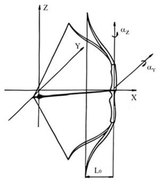
Figure 1.
Diagram of the inner ballistic trajectory of an arrow [9]. αy: the angles of a bow’s torsion around the y-axis; αz: the angles of a bow’s torsion around the z-axis; L0: the length of an initial draw.
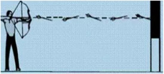
Figure 2.
Diagram of the outer ballistic trajectory of the arrow [9].
Researchers [11,12,13,14,15,16,17,18,19] have begun to study the outer ballistic trajectory of arrows only in recent years. Denny [14] estimated the lift and drag coefficients of arrows according to the geometry (size and structure) of arrows. On this basis, Zanevskyy [15] further established a complex model considering the angle between the longitudinal axis of the arrow and its flight direction, that is, the angle of attack (γ). This represents the deviation of the arrowhead from its flight path, as shown in Figure 2. Liston [16] and Park [17] modeled an arrow by dividing the arrow into four modules, namely the arrowhead, shaft, nock, and fletching, thus investigating the influences of boundary-layer transition on the shooting accuracy of the arrow. Afterwards, Park et al. [18] conducted water-channel experiments to further verify that the boundary-layer transition greatly influences the shooting accuracy of arrows. Okawa [19] measured the drag coefficients, the lift coefficients, and their relationships with the Reynolds numbers of two arrows under different initial velocities and γ by performing wind tunnel experiments and flight experiments. In this way, they verified that the shape and γ of arrowheads affect the laminar–turbulent transition in the boundary layer.
Figure 2 illustrates that the arrow’s angle of attack, γ, changes dynamically during its flight, and this variability results in a fluctuating aerodynamic center of pressure, Cp. Aerodynamics significantly affects the trajectories of sports projectiles [20,21,22,23,24,25]. For example, Maheras et al. [25] studied javelins of a larger mass and found that changes in the Cp position of javelins influence the pitch moment of javelins, thus altering their trajectory. However, arrows have a lower mass and a higher Mach number than javelins. In addition, the presence of the fletching also complicates the computation of Cp. Therefore, there is still no public literature available for detailed research on changes in the Cp in the flight process of arrows. On the contrary, military weapons and missiles of a larger mass and Mach number (0.5 to 4) have been well studied [26,27]. For example, Nielsen [26] explored the Cp position of different missiles and evaluated the influences of γ and aircraft shape on Cp. Zhang [27] discussed the aerodynamic characteristics of theater ballistic missile targets through computational fluid dynamics (CFD) simulation and wind tunnel experiments. It was found that the Cp of the ballistic missile will move forward when γ increases at supersonic velocity. Using the “×-+” fin structure will make the Cp of the “all stages” model change little when the angle of attack increases, ensuring the need for the high stability of the missile. Obviously, for any object in flight (arrows included), the center of aerodynamic pressure, Cp, as a force-bearing point changes constantly in the flight process, and its position is a non-negligible factor when predicting both the flight trajectory and attitude. Unfortunately, there are no published reports on the detailed study of the changing rules of the aerodynamic pressure center of arrows during flight. Moreover, the existing mathematical models for predicting the trajectory of an arrow’s motion are all based on classical Newtonian mechanics; that is, the point where the arrow’s aerodynamic pressure applies is regarded as fixed. This leads to low prediction accuracy and numerical calculation results. Particularly in practical competitions affected by background winds, this exerts critical influences on the performance of top athletes.
Archery competitions using recurve bows were conducted outdoors, so the influences of background winds must be considered [28,29,30]. Ando [28] found that under background winds, retaining a laminar boundary layer can significantly reduce the offset (the deviation or displacement of the arrow’s trajectory from its intended path) of arrows. Ortiz [29] quantified the influences of background winds on the aerodynamics of arrows in the flight process using a mathematical model based on information of background winds in the archery field at the 2020 Tokyo Olympic Games provided by JAMSTEC. Delaying the laminar–turbulent transition timing in the boundary layer was found to be capable of improving the resistance of arrows to wind drift. Miyazaki [30] found that the boundary-layer transition occurs if the Reynolds number of the arrow shaft is in the range of 1.2 × 10⁴ < Re < 2.0 × 10⁴. It is worth noting that they found, through experiments [31], that with a small Reynolds number, the laminar boundary layer can be well maintained if the initial γ of the arrows is kept within 3°, thus decreasing the drag coefficient.
In this study, to more comprehensively analyze the motion of arrows in the outer ballistic trajectory, COMSOL (https://cn.comsol.com/) was used at first to perform a CFD simulation of the three-dimensional (3-d) model of an arrow. Changes in Cp under different γθ (the included angle between the arrow shaft and the center of mass, Cm, velocity in the Z-direction) and different γβ values (the included angle between the arrow shaft and the Cm velocity in the Y-direction) were studied. Based on this, equations for variation in Cp with the angles were fitted. Secondly, the above equations were proposed to develop the pre-existing mathematical model in order to improve the aerodynamic model of the arrow along the outer ballistic trajectory. Thirdly, the motion trajectories and attitudes of arrows under different initial γ values and underground winds were calculated and analyzed based on the new theoretical model through MATLAB™ 2021 programming. Finally, the effects of the offset between the Cp and the Cm of the arrow on the shooting accuracy of top athletes were examined, and advice was provided to athletes.
2. Materials and Methods
2.1. Calculation Method for the Center of Aerodynamic Pressure of an Arrow
2.1.1. Main Governing Equations and Turbulence Model
The RANS method is applied to calculate the flight state of an arrow in this study. RANS has slightly lower accuracy compared to DNS and LES, but it offers higher computational efficiency [32,33,34,35]. The solution obtained using RANS can still meet practical engineering requirements, providing accurate numerical solutions even with coarser grids.
The governing equations include the mass conservation equation, momentum conservation equation, and equations describing the turbulence model.
- (1)
- The mass conservation equation iswhere is the fluid density (kg/m3); denotes the velocity vector (m/s).
- (2)
- The momentum conservation equation iswhere p, I, F, and denote the pressure (Pa), momentum vector (N∙s), vector of body force (N), and dynamic viscosity (Pa∙s), respectively.
- (3)
- Relevant equations of the RANS k-ε turbulence model are as follows.
The turbulence energy k is given by
where k is the turbulence energy (m2/s2); denotes the turbulent Prandtl number in k equation, and is the dissipation rate (m2/s3).
The dissipation rate is given by
where σε is the turbulent Prandtl number in ε equation; Cε is a constant in the model.
The turbulent viscosity coefficient is given by
where is a constant in the model.
2.1.2. Geometric and Physical Model of an Arrow
The model of the arrow studied here is an Easton X10, as shown in Figure 3. The arrow shaft is made of a composite of high-modulus carbon fiber and aluminum-alloy materials. The arrowhead is made of tungsten steel, and the fletching is made of three soft plastics, with a total mass of 1.97 × 10⁻² kg. Table 1 lists the mass (M), length (L), shaft radius (R), and blade thickness (h) of the arrow, and its three-dimensional geometric model is shown in Figure 4.
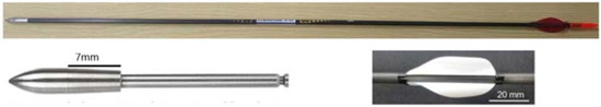
Figure 3.
Easton X10 model, X10 stainless steel break-off point and SPIN-WING-VANES (lower center).

Table 1.
Physical properties of arrows.
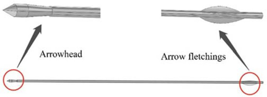
Figure 4.
Physical model of an arrow.
The angle of attack is positive when the arrow points above the velocity direction of the arrow’s center of mass (left) and negative when the arrow points below the velocity direction of the arrow’s center of mass (right), as shown in Figure 5. θ is the angle between the velocity direction of the arrow and the arrow’s center of mass. As this is subdivided into γθ and γβ during simulation, θ is used to explain the positive and negative angles of attack. Figure 6 shows the structure of the flow field, in which the air is incompressible under such a flow regime and the arrow flies within a cuboid measuring 1.5 m × 1 m × 1 m. The arrowhead is at a position some 0.5 m from the inlet; air flows in from the left and out through the right.
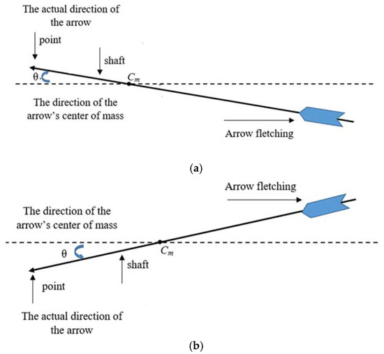
Figure 5.
A simple physical model of an arrow. (a) γ in the positive direction; (b) γ in the reverse direction.
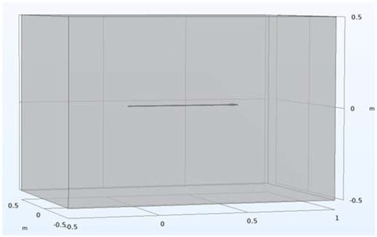
Figure 6.
Computational domain.
2.1.3. Boundary Conditions and Meshing
In 70 m archery competitions with recurve bows, elite archers typically achieve an initial arrow velocity of approximately 57 m/s. Therefore, an inlet velocity of 57 m/s was prescribed, oriented parallel to the X-axis and perpendicular to the inlet surface. At the outlet, a gauge pressure of 0 was imposed. Given that the arrow’s flight speed is less than 0.3 Mach, we modeled the air as an incompressible fluid. The simulations then utilized air material properties at 20 °C under standard atmospheric pressure. The density (ρ) was set to 1.204 kg/m3, and the dynamic viscosity (μ) was 1.813 × 10⁻5 Pa·s. The initial γ was varied within the range of [−3°, 3°] in increments of 0.1°. The influence of the arrow’s γθ and γβ on its Cp was subsequently investigated.
The computational mesh was generated using unstructured tetrahedral elements. Three refined boundary-layer grids were implemented along the arrow surface, with increased mesh density near the arrowhead and nock. Grid independence was verified by analyzing the surface pressure on the arrow. Four mesh configurations (Cases A–D) were evaluated for three different angle-of-attack (γ) values (see Table 2). As shown in Figure 7, the surface pressure exhibited minor fluctuations across different grid resolutions when the angle of attack was 0°, 1°, or 2°. Under higher angles of attack, the results obtained using the finer meshes (Cases C and D) were consistent, with differences less than 1%. To balance computational costs and accuracy, the mesh configuration corresponding to Case C was selected for subsequent simulations, and its structure is visualized in Figure 8.
Table 2.
Numbers of grid cells.
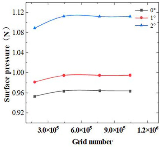
Figure 7.
Grid independence verification.
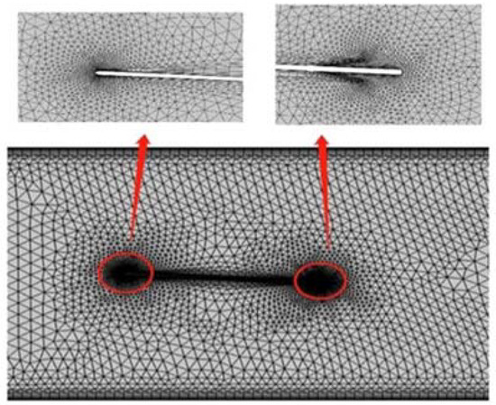
Figure 8.
Grid structure.
2.1.4. Verification of the Turbulence Model
To verify the reliability of the RANS k-ε turbulence model, the velocity field is calculated when the angle of attack is ±2.9° and ±3.0°. When the Reynolds number is 1.8 × 10⁴, the velocity contour plot is as shown in Figure 9. As the angle of attack increases to ±3.0°, the air behind the largest bulge of the arrow begins to generate backflow, causing boundary-layer separation. The simulation results are consistent with Miyazaki’s experimental results. Miyazaki [31] and others used MSBS wind tunnel experiments and free flight experiments to study the effects of arrow speed and the arrow’s initial angle of attack on the boundary-layer state on the arrow axis. Their research found that the arrow axis will produce a boundary-layer transition in the range of 1.2 × 10⁴ < Re < 2.0 × 10⁴. At a high Reynolds number, when the angle of attack is 3°, the airflow behind the arrow will separate, and reverse flow is generated. At this time, the arrow boundary layer will change from laminar flow to turbulent flow. This shows that the RANS k-ε turbulence model is suitable for subsequent research.
Furthermore, to validate the reliability of the simulation model, we reduced the initial arrow velocity to 23 m/s. At this velocity, the boundary-layer Reynolds number of the arrow was 7.7 × 10³, and we calculated the lift coefficient (CL) and pitching moment coefficient (CM) of the arrow at this Reynolds number. The simulation results were then compared with experimental data reported in the literature [31] at the same Reynolds number, as shown in Figure 9c. Both the wind tunnel experimental error and the simulation error for CL were within 10%, with an average error of 6.44% and a maximum error of 9.31%. For CM, the average error was 4.21% and the maximum error was 8.07%. These results demonstrate the reliability of the simulation model established in this study.

Figure 9.
Velocity vector of the arrow. (a) Velocity vector under γ of ±3°; (b) velocity vector under γ of ±2.9°; (c) comparison of simulation and experimental data [31].
Figure 9.
Velocity vector of the arrow. (a) Velocity vector under γ of ±3°; (b) velocity vector under γ of ±2.9°; (c) comparison of simulation and experimental data [31].

2.1.5. Processing of the Calculated Results
The following equations are needed to calculate the acting point of aerodynamic pressure:
- (1)
- The pressure coefficient at a certain point on the arrow surface iswhere p is the static pressure at the point; pinf denotes the far-field air pressure; is the far-field air density, and Vinf is the far-field air velocity.
- (2)
- The pressure vector at a certain point on the arrow surface iswhere np = (npx, npy, npz) is the normal vector component at the point.
- (3)
- The Cp position iswhere A is the surface area of the arrow; dS refers to the element area on the material surface.
Using the above equations, the Cp positions of the arrow in x, y, and z-directions can be calculated. In the simulation, Cp in the z-direction is fixed at a position 1.4 m above the ground, and that in the y-direction is the center of the diameter of the shaft. Therefore, it is necessary to calculate only those changes in Cp in the x-direction with a variation in γ.
2.2. Aerodynamics Model
2.2.1. Aerodynamics Characteristics of the Arrow
After identifying changes in the position of the center of aerodynamic pressure of the arrow through CFD, an aerodynamics model of the arrow was established to study the offset under background winds. Two previous studies [29,30] simplified the deformation of arrows during flight, assuming that significant deformations only occur during a brief period just after the arrow leaves the bow. Furthermore, according to the archer’s paradox, this deformation is believed to be conducive to hitting the target and is thought to have little effect on accuracy [1]. Therefore, we conducted a simulation of archery using rigid body equations, without considering deformation. This approach reduces the complexity of the model while preserving the accuracy of the results. The aerodynamic characteristics of the arrow used in the research were obtained by Ortiz [29] via wind tunnel experiments, as listed in Table 3. Parameters α and β are separately related to the lift and pitch moment and have two different drag coefficients, separately corresponding to the laminar and turbulent boundary layers; I is the moment of inertia vertical to the shaft, and I3 represents the moment of inertia around the shaft.
Table 3.
Aerodynamics characteristics of the arrow [29].
2.2.2. Equations of Motion
Archery under background winds was studied. The arrow model was set as a rigid body, and the deformation of the arrow in the free flight process was ignored, thus defining a fixed coordinate system (x, y, z) relative to the ground, which corresponds to the unit vectors (i, j, and k), as shown in Figure 10. In the mathematical model, the velocity of background winds and the Cm velocity of the arrow were separately set to U = (Ux, Uy, Uz) and V = (V sinΘ cosΦ, VsinΘ sinΦ, VcosΘ). The relative velocity is the vector difference between the Cm velocity of the arrow and the component of background winds or the vector difference of V – U. t = V – U/|V – U|is a unit vector that is parallel to the relative velocity and tangent with Cm of the arrow; n = (sinθ cosφ, sinθ sinφ, cosθ) is a unit vector along the axial direction of the arrow, in which θ is an included angle between n and z. The projection of n on the ground has an included angle of φ with the x-axis. Θ is an included angle between the resultant velocity of Cm of the arrow and background winds and the z-axis. Φ denotes an included angle between the projection of t on the ground and the x-axis. In the flight process, the arrow is subjected not only to gravity but also to aerodynamic drag, thus forming a torque allowing the arrow to rotate around Cm. The torque causes the resultant velocity of Cm and background winds to show an angular offset with the long axis of the arrow. The angle induced via such an offset can be defined as γ = cos – 1[n·t].
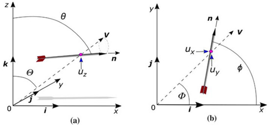
Figure 10.
Illustration of an arrow in free flight with relevant variables. (a) Schematic diagram of the x-z plane; (b) Schematic diagram of the x-y plane.
The drag (FD) and lift (FL) acting on the arrow during flight cannot be ignored. The drag occurs in the direction opposite to that of V – U, which decelerates the arrow and leads to the lateral displacement of the arrow. The lift is vertical to V – U, which results in the longitudinal displacement of the arrow. The drag and lift in the form of vectors are represented as follows [31]:
where CD is the drag coefficient, denotes the air density, α is related to the lift coefficient, and ; r is the axial radius of the arrow. These parameters are listed in Table 1 and Table 3 [24].
The angular momentum is
where w3 is the angular velocity component of the axis. The motion of the arrow can be described using the following equations [29]:
where Sp is the spin parameter, and it is obtained from wind tunnel tests. The mass and acceleration of gravity of the arrow are separately symbolized as M and g; N3 is the axial component of the torque. Parameter β is listed in Table 3, and it is related to the pitch moment and was determined through experiments.
The value of N3 cannot be determined in experiments, so an empirical assumption must be introduced, such that the angular velocity of the arrowhead under a small γ is independent of γ, and it shows a certain proportional relationship with the Cm velocity of the arrow. Additionally, the equation for Cm was obtained by fitting the above CFD data and added to the aerodynamics equations in order to more accurately assess the influences of Cm on the offset in the free flight process of the arrow.
The equation was solved using an iterative method. The time step is Δt = 5 × 10⁻⁴ s, and dv/dt, dθ/dt, dφ/dt, d2θ/dt2, d2φ/dt2, and dw3/dt need to be solved at each time step.
2.2.3. Initial Conditions
x0 = y0 = 0 and z0 = 1.5 m denote the initial position of the arrowhead. The target is at the location 1.3 m above the ground and 70 m away in the x-direction. The value of Θ0 is obtained at U = 0 when the arrow hits the target, and Φ0 = 0. The initial Cm is obtained via the fitting equation. The initial γ is changed by altering θ and φ to study the motion trajectory of the arrow. When the arrow is shot at the ideal initial angular velocity, , which means that the motion direction of the arrowhead is aligned with the resultant velocity of the Cm of the arrow and the background winds. As a result, γ is near-zero, thus maintaining the laminar boundary layer. Under this condition, the CD value of the laminar flow is used for calculation. When γ is large, the CD value of the turbulent flow is used for calculation.
A single uniform wind field and the wind only blowing in a fixed direction at a fixed velocity in the single uniform wind field were used in the research. No matter where the arrow was, it was subjected to wind (crosswind (Uy > 0), headwind (Ux < 0), or tailwind (Ux > 0)) at the same velocity. The wind power was at two scales: light air and a light breeze (1 to 3.3 m/s). Due to the influences of wind, the arrow showed a certain offset from the target center. The radial distance between the offset point and the target center is expressed as
2.2.4. Model Validation
The initial conditions for the simulation are defined as dθ/dt = dφ/dt = 0, φ0 = 0, and θ0 = Θ0. The offset of the arrow in the y-direction during flight was calculated and compared with published data [28] under identical initial conditions. As illustrated in Figure 11, the model data demonstrate an error of less than 2% compared to prior studies for Uy = 3 m/s and 1 m/s. This comparison confirms the reliability of the mathematical model used. This level of agreement demonstrates the mathematical model’s high degree of accuracy. The aerodynamic equations were implemented using MATLAB™, following the computational flowchart outlined in Figure 12.
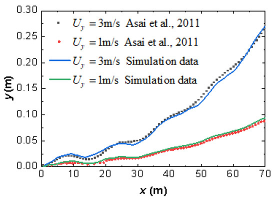
Figure 11.
Model validation [23].
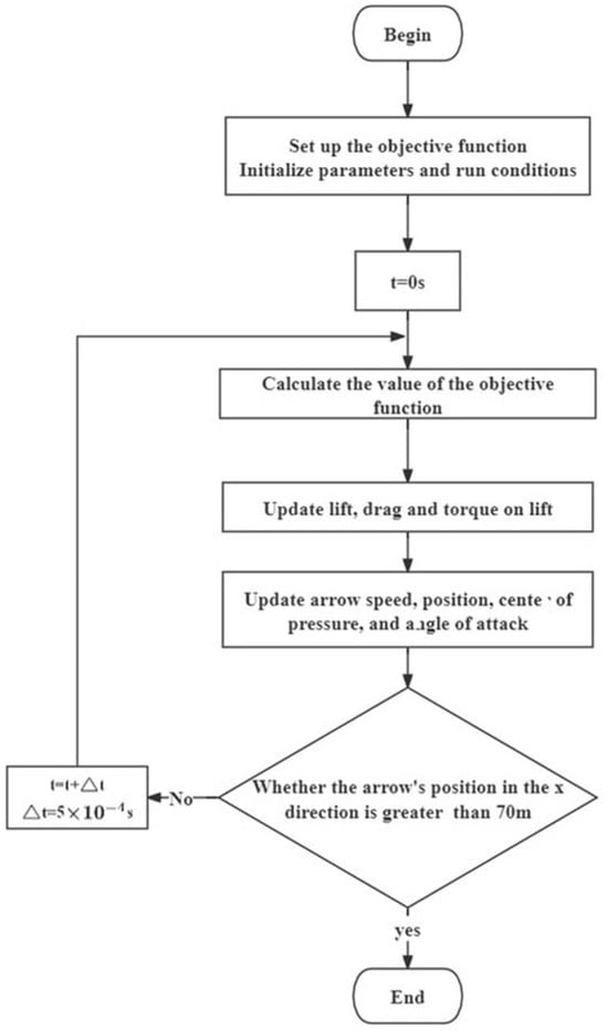
Figure 12.
Calculation flow chart.
3. Results
3.1. Influences of Changes in γ on CP
Cp and Cm positions of an arrow do not generally overlap. The offset between the Cp and Cm positions may affect the stability and flight performance of the arrow.
When the γθ and γβ change in flight, the aerodynamic moment on arrows also varies, causing differences in the force distribution on the arrow and, therefore, variation in the position of Cp. For a recurve bow, the arrow features a non-zero γ on the vertical plane when it leaves the bow, which facilitates the disengagement of the arrow from the bow, guarantees a short shooting time for the arrow in contact with the bow, and therefore maintains the stability of the arrow.
Since the arrow moves very fast, the force of air on the arrow is also very strong. It can be seen from the arrow surface pressure diagram in Figure 13 that the arrowhead and fletching are the positions that bear the greatest pressure. The frictional resistance along the arrow shaft and the resistance from the arrow fletching are the main components of the fletching force. Relative to the lift on the arrow under small γ, the vertical force on the arrowhead is small. The lift on the fletching cannot be ignored: this dominates the spin of the arrow and helps maintain flight stability, while the drag on the fletching also induces a slight, non-negligible, lateral displacement of the arrow. The specific forces acting on the arrow are shown in Figure 14.
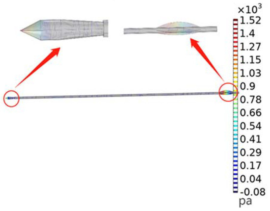
Figure 13.
Contour lines for surface pressure on the arrow. Contour line: surface pressure (Pa).
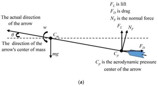
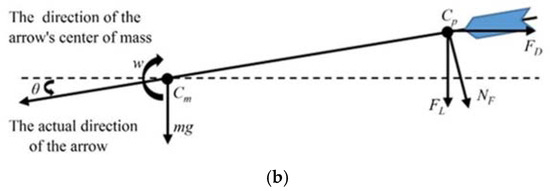
Figure 14.
The force diagram of an arrow in the air: (a) γ > 0. (b) γ < 0.
Figure 15 illustrates changes in Cp with γ, and γθ and γβ are the pitch angle and yaw angle, respectively, providing a more detailed differentiation of the attack angle, γ. γθ expresses the variation in the attack angle in the simulation with a change only in the arrow’s upward and downward angular deflection, while γβ expresses the variation in the attack angle in the simulation with a change only in the arrow’s horizontal angular deflection on the plane. In the free flight process of the arrow, Cp varies a little (by millimeters). Under the conditions of a zero and small γ, the Cp is concentrated in the nock region, ranging from 0.478 to 0.498 m. The moment (drag and lift on the fletching and on the arrow shaft to the rear of the center of mass) on the rear part of the arrow is always greater than that on the front part of the arrow (the point and the arrow shaft in front of the center of mass). When the angle of attack is large, the arrow will become unstable. Since the angle of attack of the arrow in international archery competitions generally does not exceed ±3°, the change in the pressure center point when the angle of attack is large was not studied in the present research.
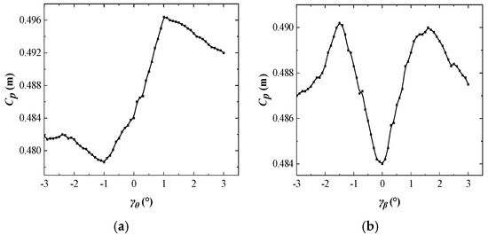
Figure 15.
(a) The relationship between Cp and γθ; (b) the relationship between Cp and γβ.
As shown in Figure 15a, Cp separately reaches its minimum and maximum values when the γθ is −1° and 1°. This is because, when γθ is negative, to align the Cm velocity with the arrowhead, the air drag on the nock turns to down-pressure, thus forcing the arrow to lift. The forward shift in the Cp position occurs to reduce the moment and therefore decelerate the lifting speed of the arrow, thus maintaining a more stable flight of the arrow. If γθ is positive, because the Cm velocity is below the flight direction, the air drag on the arrow turns to lift that is conducive to the arrow inducing a stable spinning effect, which is enhanced via the backward shift of the Cp position, thus decreasing γθ. When γθ decreases, the Cp position moves forward again, which reduces the moment on the arrow again, thus weakening the above spinning effect. This not only keeps the arrow flying more stably but also decreases the conversion of kinetic energy to maintain a high flight velocity for the arrow. The Cp position changes more slowly when γθ exceeds ±1° and gradually shifts to that when γθ is zero. The phenomenon is probably related to the fletching and boundary layer. Of course, the arrow is likely to be unstable with a large γθ so that it rapidly raises its head or drops.
The changes in the Cp position with γβ are illustrated in Figure 15b. Cp is distributed symmetrically positively and negatively with a zero γβ as the boundary. The Cp position gradually shifts backward when γ is in the range of 0° to ±1.5°, and it reaches the largest value when γβ is ±1.5°, followed by gradual forward movement, while at a speed slower than that under small γβ (0 to ±1.5°). The difference with the case of γβ is that, either during leftward or rightward deflection, the Cp position always shifts backward at first with a small γβ. This enhances the force on the rear part, reduces deflection, and therefore decreases the lateral displacement of the arrow. The peak appears at a position some 0.5° larger than that in the case of the γβ, probably because the arrow is not affected by the gravity on the lateral plane so that the position of Cp varies slightly.
Cp and γ are fitted using an empirical equation, as illustrated in Figure 16: Figure 16a,b demonstrate that the fitting curves are similar to the raw data; the residual error graphs of Figure 16c,d also show that points are distributed around the curves, suggesting that points on the fitting curves can approximately represent the raw data.

Figure 16.
Fitting curves and residual error graphs. (a) γθ fitting curve; (b) γβ fitting curve; (c) γθ residual plot; (d) γβ residual plot.
In these equations, γθ and γβ are independent variables, Cp is the dependent variable, and the remaining symbols are constants.
Equation parameters are listed in Table 4. The equation was applied to the mathematical model to explore the trajectory of the arrow during free flight.
Table 4.
Fitting equation parameters.
3.2. Arrow Behaviors Under Uniform Background Winds
3.2.1. Influences of the Arrow Mass on the Shooting Accuracy
As illustrated in Figure 17, when the initial velocity is 57 m/s, the offset of the arrow on the target decreases constantly with the increasing mass of the arrow, regardless of the initial γ, initial angular velocity, and changes in wind velocity. This means that a heavier arrow achieves better resistance to wind drift, while the effect decreases with increasing mass. When the arrow weighs 0.0142 kg and has an initial angular velocity of 0, and the crosswind velocities are 1 and 3 m/s, the offsets are respectively 0.12 and 0.322 m, which means that an arrow with a lower mass is more easily affected in flight by external factors, including wind power. As a result, the offset is more greatly affected. When the arrow weighs 0.0197 kg, the offset separately decreases by 0.02 and 0.048 m when the crosswind velocities are 1 and 3 m/s, indicating that, when the arrow is lighter and the wind velocity is high, slightly increasing the mass of the arrow can reduce the wind drift.
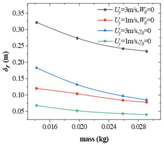
Figure 17.
The relationship between the arrow mass and the offset.
When the arrow weighs 0.0291 kg and the initial angular velocity is 0, the offsets of the arrow under the same crosswind are 0.078 and 0.229 m, which are much smaller than those of the arrow weighing 0.016 kg. This is because the heavier the arrow, the greater the inertia, and the weaker the influences of external factors in flight. As a result, the offset is slightly influenced. If the arrow mass is decreased by 0.0032 kg, the offsets respectively increase by 0.006 and 0.013 m. Therefore, tiny changes in mass exert slight influences on the offset of the arrow if the arrow is heavier: under these conditions, what must be noted is that the arrow and bow should be matched. If the arrow is light while the bow is powerful, the arrow may deviate due to the excessive centripetal force generated when it is shot. On the contrary, if the strength of the bow is too low, the arrow probably cannot be accelerated to a sufficient velocity and distance, thus failing to reach the expected accuracy and quality of a shot.
3.2.2. Changes in the Offset
Figure 18 shows the offset of the arrow on the target and the radial offset in the flight process with time. As shown in Figure 18a, when the initial velocity is 57 m/s, the Uy is 3 m/s, and the initial angular velocity is zero, the offset reaches the maximum of δr = 0.27 m, while δr is 0.125 m when the initial γ is zero. This implies that γ significantly affects the offset in the presence of background winds. This is probably because, when the initial angular velocity is zero, the initial γ is 3°, and the boundary layer of the arrow becomes turbulent, which applies more drag, thus increasing the lateral displacement. Therefore, controlling the initial attack angle is a crucial strategy to help athletes improve their scores. When the crosswind speed (Uy) is 2 m/s, the maximum deviation is 0.16 m, which is 0.1 m less than the deviation observed at 3 m/s. This finding indicates that the magnitude of the crosswind has a significant effect on the arrow’s trajectory, confirming that, under crosswind conditions, the deviation is caused by the lateral component of the drag force, FD. The magnitude of wind velocity also affects the boundary-layer state of the arrow: the larger the wind velocity, the greater the drag on the arrow.
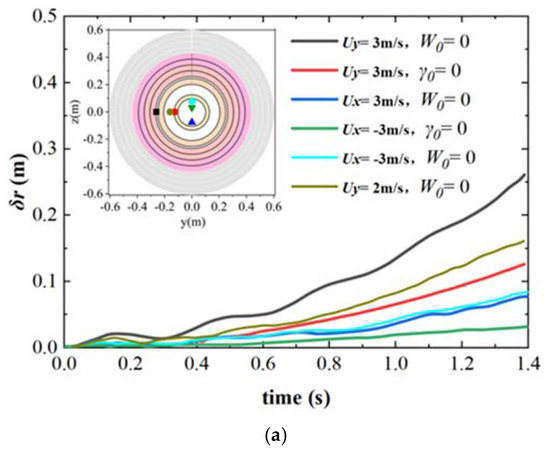
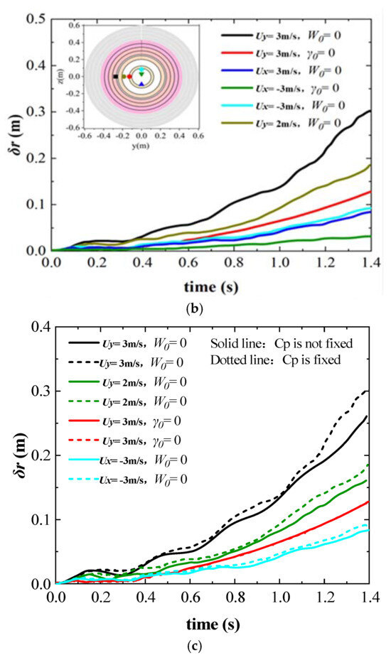
Figure 18.
Changes in the offset. (a) Changes in the offset with time; (b) changes in the offset with time under the fixed Cp position; (c) comparison of the offsets.
When Ux = 3 m/s, the maximum deviation is 0.077 m, which is 0.2 m less than the deviation caused by crosswind at the same wind speed. However, when the wind changes to a headwind, the deviation increases by approximately 0.007 m. This increase is attributable to the headwind’s enhancement of the arrow’s air resistance, leading to a slightly larger deviation than under tailwind conditions. However, because the largest γ is 0.49° under headwind conditions, Cp remains stable in flight, and boundary-layer transition does not occur. The drag is low so that the offset is much smaller than that under crosswind. This also demonstrates that the crosswind affects the arrow more than headwind and tailwind.
To illustrate the unique characteristic of the pressure center continuously varying with the arrow’s motion, this study also examined the deviation of the arrow when the pressure center is fixed. As shown in Figure 18b, the variation in the arrow’s deviation is shown with the pressure center fixed at 0.484 m, and a comparison with varying pressure center conditions is presented in Figure 18c. When the crosswind velocities are 3 and 2 m/s and the initial γ is not zero, the offsets of the arrow are separately 0.306 and 0.185 m, which separately increase by 0.04 and 0.02 m compared with those when CP is not fixed. This greatly influences the scores in archery competitions. In the case of headwind, the deviation is increased by 0.008 m compared to when the pressure center varies with arrow movement. This difference is significant and cannot be ignored. It further implies that the small variation in the pressure center in flight benefits the overall force on the arrow, thus improving accuracy.
With an initial angular velocity of zero, the deviations are quantified in Table 5. This table presents the specific deviation values for both models across different wind conditions. In the context of archery, the mental fortitude and release stability of top athletes are undeniable. If these factors are excluded, an accurate assessment of the background wind and the corresponding scientific adjustments to the archer’s posture are key determinants of performance. In contrast to previous research, and according to our new, more precise computational model, the adjustment strategies for athletes are as follows: Under crosswind conditions, the accuracy of the non-Cp-fixed model improves by approximately 15% relative to the Cp-fixed model. Similarly, in headwind and tailwind conditions, the accuracy increases by around 8%.
Table 5.
W0 = 0, δr of two models under background wind.
3.2.3. Changes in Cp and γ
Figure 19 shows changes in the Cp and γ of the arrow with time in free flight: γ varies at a certain frequency in the flight process, and such fluctuation causes constant changes in the Cp position, which gradually reduces the amplitude of fluctuations of γ. This is because the arrow is subjected to the pitch moment, which aligns the arrow with the airflow. If no lift is applied to the arrow in the process, the changes in the γ and Cp position will fluctuate at a fixed frequency. When Uy is 3 m/s and the initial angular velocity is zero, the γ and Cp position change significantly, leading to unstable forces on the arrow. Under these conditions, the boundary layer of the arrow may undergo a laminar–turbulent transition, increasing the drag and reducing the accuracy of the shot.
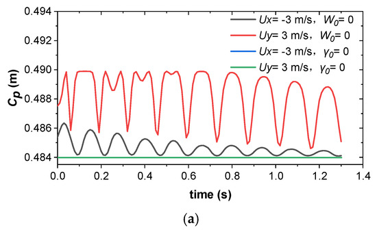
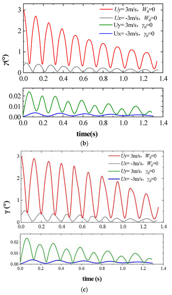
Figure 19.
Changes in Cp and γ. (a) Changes in Cp with time; (b) changes in γ with time; (c) changes in γ with time when Cp is fixed.
The variation in the angle of attack is also calculated when Cp is fixed. As shown in Figure 19c, when Cp is fixed at 0.484 m and the initial angular velocity is zero, the fluctuation amplitude of γ is much greater than that when Cp varies, and the rate of amplitude attenuation is low. Particularly when Uy = 3 m/s, γ changes slightly, thus increasing the offset of the arrow. If the initial γ is zero, changes in γ differ slightly from those when the Cp position varies. Therefore, maintaining Cp within a certain range in arrow design can not only improve shooting accuracy but also decrease the sensitivity of the arrow to initial conditions, thus making it easier for archers to hit the target.
Under a crosswind, the γ and Cp of the arrow fluctuate more than those under tailwind and headwind conditions, implying that the arrow wobbles more under crosswind conditions and thus leading to a larger offset. If the initial γ is zero, the amplitude of fluctuation is small throughout the flight and Cp is stable, so the boundary layer of the arrow remains laminar. This reduces the drag and contributes to the higher shooting accuracy of the arrow. Hence, controlling the initial γ and initial angular velocity is extremely important to archers.
3.2.4. Influences of the Cm Position on Shooting Accuracy
When keeping the total mass unchanged, the distance between Cm and Cp also greatly affects the accuracy of the shot. As shown in Figure 20, when Cm is 0.185 m from the arrowhead, a crosswind at 3 m/s is applied, and the initial γ is 0°, the offset on the target is 0.116 m. If Cm is shifted backwards to 0.2 m, the offset increases by 0.03 m. The result indicates that the further forward Cm is, the more accurate the shot. Even if the initial γ is zero and the overall disturbance to the arrow is low, the offset can be decreased by changing the Cm position.
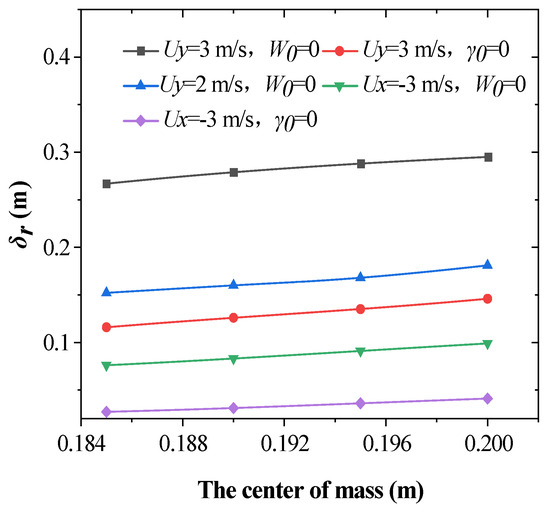
Figure 20.
Changes in the offset with the Cm position.
The offset increases by 0.026 m with the backward shift in Cm when the crosswind velocity is 3 m/s and the initial angular velocity is zero. The value is lower than that under the initial γ of 0°. This suggests that the closer the Cm is to the arrowhead, the greater the corrective moment applied via the fletching and the better the correctability and stability. However, within medium and long shooting ranges, the further forward the Cm is, the more obvious the bending and falling of the trajectory at the end. Under these conditions, the initial shooting angle needs to be adjusted, and the accuracy of the shot becomes more sensitive to the initial shooting velocity and shooting angle, which calls for excellent shooting skills. If the Cm of the arrow is shifted backwards, the corrective moment and the resistance to wind drift are low: under these conditions, the accuracy of the shot becomes less sensitive to the initial shooting conditions.
3.3. Practical Performance and Adjustment Strategies for Athletes on the Archery Field
Figure 21 presents target images from both the Chinese and Korean archery teams. From these images, it is evident that crosswind significantly affects the scores of archers from both teams. On the day in question, there was a right crosswind of approximately 2 m/s, accompanied by a headwind of around 2 m/s. The arrow located at the upper left corner of Figure 21a and the one on the left in Figure 21b represent the first shots. They have δr values of 0.12 m and 0.125 m, respectively. Without concrete data to guide their adjustments, the athletes could not gauge the precise arrow deviations for the given wind speed. Consequently, this scenario more closely mirrors the maximum δr deviation of 0.161 m, as projected by the model developed in this research for a 2 m/s crosswind. This alignment suggests that our proposed model is more accurate than the fixed Cp model. The three arrows on the right-hand side of Figure 21b represent subsequent adjustments made by the athletes after their initial shots. These modifications led to rightward deviations of 0.08 m and 0.13 m, which were not optimal results. According to the model presented in this study, adjusting the initial θ to 87.8° and the initial φ to −0.9° could keep the deviation within 0.06 m, showing a more accurate adjustment compared to the athletes’ attempts.
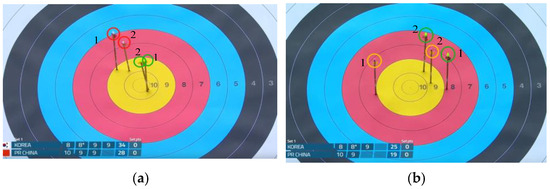
Figure 21.
Archery World Cup Shanghai Station target images. (a) Target image for team China; (b) Target image for team Korea.
As shown in Figure 22, it is clear that the arrows are more influenced by headwinds and tailwinds than by crosswinds. The majority of the arrows lie either above or below the target’s center. On this day, the conditions included a crosswind of around 1 m/s and a headwind close to 4 m/s. In Figure 22a,b, the arrows furthest from the target’s center signify the initial shots, showcasing δr values of 0.13 m and 0.12 m, respectively. Side deviations were minimal, at 0.08 m and 0.03 m for left and right, respectively. The deviation in this wind condition, as compared to the present model data, is off by about 0.03 m. This represents an 8% increase in accuracy over previous models, offering athletes a more accurate reference. Athletes then adjusted their shots based on these vertical deviations. In Figure 22a, these adjustments proved suboptimal, with notable deviations remaining. According to our study, tweaking the initial θ to 86.3° and the initial φ to 0.3°—essentially aiming for a near-zero initial attack angle—could minimize the deviation by 0.10 m. Athletes, armed with the wind deviation data from our research, can fine-tune their arrow’s initial angle to better counter wind-induced effects, thereby increasing their potential score.
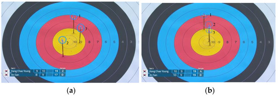
Figure 22.
Archery World Cup Shanghai semi-final target images. (a) Target image for Kang Chae Young, Korea; (b) Target image for An San, Korea.
4. Conclusions
The attitude of the arrow during free flight was simulated via CFD, and the aerodynamics model was established with a consideration of the influences of Cp and uniform background winds. The following conclusions can be drawn by analyzing the results.
- (1)
- Cp is located towards the rear of the arrow and varies with the angle of attack (γ). Such variation manifests as increases or decreases of several millimeters, and it reaches a maximum of 0.496 m when γθ = 1°. Keeping Cp stable and backwards is key to reducing the offset.
- (2)
- A uniform crosswind affects an arrow more significantly than a uniform headwind or tailwind. Furthermore, within a specific range, either increasing the mass of the arrow or shifting its center of mass forward (while maintaining a constant arrow length and wind speed) can enhance the arrow’s resistance to wind deflection.
- (3)
- An improvement in the initial shooting conditions plays a significant role in reducing the offset. When the arrow is shot under zero γ, the Cp of the arrow can remain stable in flight, and the boundary layer remains laminar, thus improving the accuracy of the shot.
- (4)
- Compared to the model with a fixed Cp, the model introduced in this study has improved its accuracy by 15% under crosswind conditions and by 8% under headwind/tailwind conditions. The data from this research can help athletes more accurately predict arrow deviations and adjust their techniques accordingly.
Author Contributions
Conceptualization, X.X. and J.Z.; methodology, W.S. and L.H.; software, L.H. and Y.X.; validation, W.S., L.H. and J.H.; formal analysis, W.S. and L.H.; investigation, L.H. and J.H.; resources, Y.X.; data curation, W.S. and L.H.; writing—original draft preparation, W.S. and L.H.; writing—review and editing, Y.X., X.X. and J.Z.; visualization, W.S. and L.H.; supervision, J.Z.; project administration, J.Z.; funding acquisition, J.Z. All authors have read and agreed to the published version of the manuscript.
Funding
This research was funded by the National Natural Science Foundation of China (Grant No. 61871200) and the Natural Science Foundation of Fujian Province, China (Grant No. 2021J10854).
Data Availability Statement
The original contributions presented in this study are included in the article. Further inquiries can be directed to the corresponding author.
Conflicts of Interest
The authors declare no conflicts of interest.
Nomenclature
The following symbols are used in this manuscript:
| CFD | Computational fluid dynamics |
| Cp | Center of aerodynamic pressure |
| Cm | Center of mass |
| γ | Angle of attack |
| αy | The angles of a bow’s torsion around the y-axis |
| αz | The angles of a bow’s torsion around the z-axis |
| L0 | The length of an initial draw |
| Re | Reynolds number |
| γθ | The included angle between the arrow shaft and center of mass, Cm, velocity in the Z-direction |
| γβ | The included angle between the arrow shaft and Cm velocity in the Y-direction |
| ρ | Fluid density (kg/m3) |
| u | Fluid velocity (m/s) |
| p | Pressure (Pa) |
| F | Body force (N) |
| μ | Dynamic viscosity (Pa∙s) |
| k | Turbulence energy (m2/s2) |
| σK | Turbulent Prandtl number in k equation |
| ε | Dissipation rate (m2/s3) |
| σε | Turbulent Prandtl number in ε equation |
| μT | Turbulent viscosity coefficient |
| θ | The included angle between the velocity direction of the arrow and the arrow’s center of mass |
| CL | Lift coefficient |
| CM | Pitching moment coefficient |
| Pc | Pressure coefficient |
| pinf | The far-field air pressure (Pa) |
| ρinf | The far-field air density (kg/m3) |
| Vinf | the far-field air velocity (m/s) |
| Pvec | Pressure vector |
| A | The surface area of the arrow (m2) |
| Sp | Spin parameter |
| CD | Drag coefficient |
| I | Moment of inertia |
| FD | Drag force (N) |
| FL | Lift force (N) |
| δr | Offset (m) |
References
- Park, J.L. Arrow behavior in free flight. Proc. Inst. Mech. Eng. Part P J. Sports Eng. Technol. 2011, 225, 241–252. [Google Scholar]
- Ortiz, J.; Serino, A.; Hasegawa, T.; Onoguchi, T.; Maemukai, H.; Miyazaki, T.; Sugiura, H. Experimental and Computational Study of Archery Arrows Fletched with Straight Vanes. Proceedings 2020, 49, 56. [Google Scholar] [CrossRef]
- Kuch, A.; Debril, J.F.; Tizzoni, J.M.; Laguillaumie, P.; Monnet, T. A study of the influence of arrow mass on ballistics. Comput. Methods Biomech. Biomed. Eng. 2019, 22, S526–S528. [Google Scholar] [CrossRef]
- Hickman, C.N. The dynamics of a bow and arrow. J. Appl. Phys. 1937, 8, 404–409. [Google Scholar] [CrossRef]
- Klopsteg, P.E. Bows and Arrows: A Chapter in the Evolution of Archery in America; Smithsonian Institution: Washington, DC, USA, 1963. [Google Scholar]
- Pekalski, R. An improved archery simulator for objective dynamic tests of bows and arrows. J. Biomech. 1987, 20, 818. [Google Scholar] [CrossRef]
- Kooi, B.W.; Sparenberg, J.A. On the mechanics of the arrow: Archer’s Paradox. J. Eng. Math. 1997, 31, 285–303. [Google Scholar] [CrossRef]
- Park, J.L. Arrow behaviour in the lateral plane during and immediately following the power stroke of a recurve archery bow. Proc. Inst. Mech. Eng. Part P J. Sports Eng. Technol. 2013, 227, 172–183. [Google Scholar] [CrossRef]
- Pekalski, R. Experimental and theoretical research in archery. J. Sports Sci. 1990, 8, 259–279. [Google Scholar] [CrossRef]
- Kooi, B.W. On the mechanics of the modern working-recurve bow. Comput. Mech. 1991, 8, 291–304. [Google Scholar] [CrossRef]
- Goff, J.E. A review of recent research into aerodynamics of sport projectiles. Sports Eng. 2013, 16, 137–154. [Google Scholar] [CrossRef]
- Ertan, H. Exploratory spatial analysis of hit distribution in archery. Int. J. Acad. Res. 2013, 5, 112–118. [Google Scholar] [CrossRef]
- Kooi, B.W. Bow-arrow interaction in archery. J. Sports Sci. 1998, 16, 721–731. [Google Scholar] [CrossRef] [PubMed]
- Sawada, H.; Umezawa, K.; Yokozeki, T.; Watanabe, A.; Otsu, T. Wind tunnel test of Japanese arrows with the JAXA 60-cm magnetic suspension and balance system. Exp. Fluids 2012, 53, 451–466. [Google Scholar] [CrossRef]
- Zanevskyy, I. Mechanical and mathematical modeling of sport archery arrow ballistics. Int. J. Comput. Sci. Sport 2008, 7, 40–49. [Google Scholar]
- Liston, T.L. Physical Laws of Archery; Liston & Associates: Village, CA, USA, 1991. [Google Scholar]
- Park, J.L. The aerodynamic drag and axial rotation of an arrow. Proc. Inst. Mech. Eng. Part P J. Sports Eng. Technol. 2011, 225, 199–211. [Google Scholar] [CrossRef]
- Park, J.L.; Hodge, M.R.; Al-Mulla, S.; Sherry, M.; Sheridan, J. Air flow around the point of an arrow. Proc. Inst. Mech. Eng. Part P J. Sports Eng. Technol. 2013, 227, 64–69. [Google Scholar] [CrossRef]
- Okawa, K.; Komori, Y.; Miyazaki, T.; Taguchi, S.; Sugiura, H. Free flight and wind tunnel measurements of the drag exerted on an archery arrow. Procedia Eng. 2013, 60, 67–72. [Google Scholar] [CrossRef][Green Version]
- Iftikhar, S.; Sherbaz, S.; Haider Sehole, H.A.; Maqsood, A.; Mustansar, Z. Large eddy simulation of the flow past a soccer ball. Math. Probl. Eng. 2022, 2022, 3455235. [Google Scholar] [CrossRef]
- Rasmussen, J.; Zee, M.D. A Simulation of the effects of badminton serve release height. Appl. Sci. 2021, 11, 2903. [Google Scholar] [CrossRef]
- Alam, F.; Chowdhury, H.; Theppadungporn, C.; Subic, A. Measurements of aerodynamic properties of badminton shuttlecocks. Procedia Eng. 2010, 2, 2487–2492. [Google Scholar] [CrossRef]
- Asai, T.; Kamemoto, K. Flow structure of knuckling effect in footballs. J. Fluids Struct. 2011, 27, 727–733. [Google Scholar] [CrossRef][Green Version]
- Clanet, C. Sports ballistics. Annu. Rev. Fluid Mech. 2015, 47, 455–478. [Google Scholar] [CrossRef]
- Maheras, A. The Javelin: Basic Javelin Aerodynamics and Flight Characteristics (Part 1). Tech. Track Field Cross Ctry. 2013, 7, 30. [Google Scholar]
- Ocokoljic, G.J.; Rasuo, B.P.; Bengin, A.C. Aerodynamic shape optimization of guided missile based on wind tunnel testing and computational fluid dynamics simulation. Therm. Sci. 2017, 21, 1543–1554. [Google Scholar] [CrossRef]
- Zhang, W.; Wang, Y.; Liu, Y. Aerodynamic study of theater ballistic missile target. Aerosp. Sci. Technol. 2013, 24, 221–225. [Google Scholar] [CrossRef]
- Ortiz, J.; Ando, M.; Murayama, K.; Miyazaki, T.; Sugiura, H. Computation of the trajectory and attitude of arrows subject to background wind. Sports Eng. 2019, 22, 7. [Google Scholar] [CrossRef]
- Ortiz, J.; Ando, M.; Miyazaki, T. Numerical simulation of wind drift of arrows on the Olympic venue for Tokyo 2020. Athens J. Sports 2020, 7, 1–20. [Google Scholar] [CrossRef]
- Miyazaki, T.; Mukaiyama, K.; Komori, Y.; Okawa, K.; Taguchi, S.; Sugiura, H. Aerodynamic properties of an archery arrow. Sports Eng. 2013, 16, 43–54. [Google Scholar] [CrossRef]
- Miyazaki, T.; Matsumoto, T.; Ando, R.; Ortiz, J.; Sugiura, H. Indeterminacy of drag exerted on an arrow in free flight: Arrow attitude and laminar-turbulent transition. Eur. J. Phys. 2017, 38, 064001. [Google Scholar] [CrossRef][Green Version]
- Kumar, G.; Natale, G. Settling dynamics of two spheres in a suspension of Brownian rods. Phys. Fluids 2019, 31, 073104. [Google Scholar] [CrossRef]
- Cai, S.G.; Mozaffari, S.; Jacob, J.; Sagaut, P. Application of immersed boundary based turbulence wall modeling to the Ahmed body aerodynamics. Phys. Fluids 2022, 34, 095106. [Google Scholar] [CrossRef]
- Passiatore, D.; Sciacovelli, L.; Cinnella, P.; Pascazio, G. Finite-rate chemistry effects in turbulent hypersonic boundary layers: A direct numerical simulation study. Phys. Rev. Fluids 2021, 6, 054604. [Google Scholar] [CrossRef]
- Kan, K.; Li, H.; Yang, Z. Large eddy simulation of turbulent wake flow around a marine propeller under the influence of incident waves. Phys. Fluids 2023, 35, 055124. [Google Scholar]


Disclaimer/Publisher’s Note: The statements, opinions and data contained in all publications are solely those of the individual author(s) and contributor(s) and not of MDPI and/or the editor(s). MDPI and/or the editor(s) disclaim responsibility for any injury to people or property resulting from any ideas, methods, instructions or products referred to in the content. |
© 2025 by the authors. Licensee MDPI, Basel, Switzerland. This article is an open access article distributed under the terms and conditions of the Creative Commons Attribution (CC BY) license (https://creativecommons.org/licenses/by/4.0/).