Article

A Multiscale CNN-Based Intrinsic Permeability Prediction in Deformable Porous Media

1
Institute of Mechanics and Computational Mechanics (IBNM), Leibniz University Hannover, 30167 Hanover, Germany
2
Institute of Applied Mechanics, University of Stuttgart, 70569 Stuttgart, Germany
*
Author to whom correspondence should be addressed.
Appl. Sci. 2025, 15(5), 2589; https://doi.org/10.3390/app15052589
Submission received: 19 January 2025 / Revised: 23 February 2025 / Accepted: 25 February 2025 / Published: 27 February 2025
(This article belongs to the Special Issue Machine Learning in Multi-scale Modeling)

Abstract

:
This work introduces a novel application for predicting the macroscopic intrinsic permeability tensor in deformable porous media, using a limited set of μ -CT images of real microgeometries. The primary goal is to develop an efficient, machine learning (ML)-based method that overcomes the limitations of traditional permeability estimation techniques, which often rely on time-consuming experiments or computationally expensive fluid dynamics simulations. The novelty of this work lies in leveraging convolutional neural networks (CNNs) to predict pore-fluid flow behavior under deformation and anisotropic flow conditions. The approach utilizes binarized CT images of porous microstructures to predict the permeability tensor, a crucial parameter in continuum porous media flow modeling. The methodology involves four steps: (1) constructing a dataset of CT images from Bentheim sandstone at varying volumetric strain levels; (2) conducting pore-scale flow simulations using the lattice Boltzmann method (LBM) to obtain permeability data; (3) training the CNN model with processed CT images as inputs and permeability tensors as outputs; and (4) employing techniques like data augmentation to enhance model generalization. Examples demonstrate the CNN’s ability to accurately predict the permeability tensor in connection with the deformation state through the porosity parameter. A source code has been made available as open access.

1. Introduction

The study of single- and multiphase flow in deformable and possibly fractured porous materials is a topic of interest in various fields, such as petroleum engineering, hydrology, soil science, and biomechanics. Related applications and references can be found in, e.g., Ehlers [1], Ehlers et al. [2], Mosthaf et al. [3], Markert et al. [4], Markert [5], Ehlers and Wagner [6], Heider [7], Peters et al. [8], Miehe and Mauthe [9], Gawin et al. [10], Wang and Sun [11], Choo and Borja [12], Jenny et al. [13]. The understanding and accurate mathematical description of fluid flow in these media is crucial for optimizing extraction processes, predicting contaminant transport, improving soil irrigation techniques, and predicting the stability of geotechnical structures, among others. However, the inherent heterogeneity and anisotropy of porous media pose a major challenge to the accurate prediction of their macroscopic properties, such as permeability. This underlines the need to incorporate the microscopic information through an accurate but computationally efficient multiscale approach.
In recent years, machine learning (ML), particularly artificial neural networks (ANN) has emerged as a promising tool to tackle several problems in multiscale material modeling. Using, e.g., deep neural networks (DNN), constitutive models based on lower-scale simulations can be found in different research works, such as within crystal plasticity [14,15], elasto-plasticity for multiphase, composite materials [16], fracture mechanics [17,18], hyperelasticity with enforced constitutive restrictions, as the symmetry of the stress tensor, objectivity, material symmetry, polyconvexity, and thermodynamic consistency [19], and other applications in [20]. A recent review on ML applications within solid mechanics was presented by Jin et al. [21]. Within multiscale modeling of porous materials, ANN, including convolutional neural networks (CNNs) and regression models, have demonstrated their ability to learn complex patterns and relationships. This made them suitable for predicting macroscopic properties and material models, such as anisotropic permeability, retention curves of unsaturated porous materials, and inelastic stress–strain relationships (see, e.g., [22,23,24,25,26,27] for an overview). Specifically, the CNN approach holds significant capabilities in linking information across scales and in model parameter prediction within computational mechanics, as highlighted, for example, by Bishara et al. [28], Herrmann and Kollmannsberger [29]. The application of ML in this context has the potential to significantly reduce the computational costs associated with traditional multiscale simulation methods while ensuring a higher degree of accuracy in comparison with phenomenological models. However, the good performance of these surrogate models requires a sufficient amount of data, e.g., small-scale CT images or numerical data. If the available image database is small, data enhancement techniques can help to overcome this challenge. For example, Nguyen et al. [30] have used generative adversarial networks (GAN) together with actor-critic (AC) reinforcement learning to synthesize realistic and controlled 3D microstructures, which are also used in this work.
For the macroscopic simulation of multiphase, heterogeneous, and deformable porous materials, the theory of porous media (TPM) can be employed, which represents a reliable and robust framework, as has been demonstrated in many works, e.g., [6,31,32,33,34,35]. In this context, important parameters, such as deformation-dependent intrinsic permeability, relative permeabilities, and the degree of saturation in relation to capillary pressure, determine flow behavior in continuum multiphase porous media models. Unlike in phenomenological models and their assumptions, these parameters and the associated constitutive formulations can be estimated based on lower-scale flow simulations. For instance, the lattice Boltzmann method (LBM) can be applied to simulate the flow on the microscale through representative volume elements (RVEs) of the analyzed material. For model details and references, see, e.g., [11,33,36,37]. The implementation of LBM is a common practice in computational fluid dynamics, especially for handling complex boundaries of heterogeneous porous materials. In this context, Zhang et al. [38] explored the integration of LBM and the discrete element method (DEM) to simulate fluid–particle interactions, highlighting the importance of iterative testing to ensure that synthetic data accurately reflect real-world permeability behavior.
A study by Yang et al. [39] reviewed current advancements in data-driven approaches for analyzing flow and transport in porous media. A special focus was placed on methodologies like image-based techniques, data-driven flow modeling, and physics-informed machine learning, offering insights into their applications and future research directions. Jiao et al. [40] explored four hybrid physics-machine learning (ML) methods for predicting fracture properties in porous media: residual modeling, which refines predictions by learning model errors; integrated coupling, where a physical model’s output feeds into an ML model; simple averaging, which blends predictions from both models; and bootstrap aggregating, an ensemble approach leveraging multiple physical models. Their comparison found residual modeling to be the most effective, offering superior predictive performance. The paper by Chen et al. [41] introduced a physics-informed CNN model that leverages transfer learning to simulate two-phase flow in porous media under time-varying controls. The approach enhanced simulation efficiency and accuracy, particularly in scenarios with dynamic boundary conditions.
Within ML-based multiscale modeling of flow through porous materials, regression models using simple feed-forward neural networks (FFNN) are successfully utilized by Heider et al. [23] and Chaaban et al. [25] for capturing the time-independent permeability tensor. On the other hand, path-dependent responses, such as the retention model, could be captured using the recurrent neural networks (RNN) or the one-dimensional (1D) convolutional neural networks (1D-CNN), as thoroughly discussed in [23,25]. While the aforementioned FFNN regression models use only the LBM datasets, in this work, we discuss the use of two-dimensional (2D) convolutional neural networks (CNN) to predict the macroscopic anisotropic permeability tensor at different deformation states. From an implementation perspective, the FFNN model can bypass the explicit determination of the permeability tensor and instead directly replace Darcy’s law within the macroscopic model of porous media. In contrast, the proposed CNN is designed to predict the permeability tensor as an effective property for macroscopic modeling. The supervised learning process in the proposed CNN model uses binarized CT images of real microgeometry as inputs, while the output is the second-order symmetric intrinsic permeability tensor. Figure 1 illustrates the major steps in this model, which include building the dataset based on CT images from Bentheim sandstone and training the 2D CNN model with the processed CT images as inputs and permeability tensors as outputs.
This CNN-based treatment has shown its effectiveness in various studies, such as within multiscale magnetostatics [42] and multiscale modeling of heterogeneous materials [43].
After this introduction, the rest of the paper is organized as follows: Section 2 presents the fundamentals of macroscopic modeling of saturated porous media based on the TPM. This section covers the concepts of homogenization, kinematics, local balance relations, and essential constitutive relations for biphasic porous materials. Additionally, it reviews modeling the flow through porous media, including Darcy and Darcy–Brinkman models [1]. This is followed in Section 3 by a discussion of the data generation steps. This includes image data processing through binarization and sampling, as well as the application of the LBM for single-phase flow to compute the intrinsic permeability components. Section 4 presents the initial CNN model used in this study. It begins with a description of the model’s architecture, data preparation for training, and hyperparameter selection. This is followed by an analysis of the model’s training results and its performance on unseen data. The extension to an informed CNN model, achieved by incorporating physical parameters into the model’s architecture, and its impact on model performance are discussed in Section 5. In Section 6, an alternative approach to improving the model’s performance and generalization through data augmentation is discussed. Specifically, it begins with training an initial model on synthetic data generated via GAN to capture general patterns. This is followed by applying transfer learning, where the pre-trained model is fine-tuned on the original dataset to enhance its performance. Finally, concluding remarks are given in Section 8.

2. Macroscopic Saturated Porous Media Model

2.1. Homogenization, Volume Fractions, and Densities

For the continuum mechanical description, the following formulations consider a saturated, two-phase porous material consisting of a materially incompressible solid but compressible solid matrix and a materially incompressible pore fluid. The microscopically heterogeneous porous materials can be well described within the macroscopic TPM framework. Hereby, a homogenization process is applied to a representative elementary volume (REV), resulting in a smeared-out continuum φ with overlapping, interacting, and statistically distributed solid and liquid aggregates φ α ( α = S for the solid phase and α = F for the pore-liquid phase). See [31] for details. Having immiscible solid and fluid aggregates, the volume fraction n α : = d v α / d v of φ α is defined as the ratio of the partial volume element d v α to the total volume element d v of φ . Furthermore, the saturation constraint of the fully saturated material is expressed as
α n α = n S + n F = 1 with n S : solidity , n F : porosity .
Two density functions are also defined, namely a material (effective or intrinsic) density ρ α R : = d m α / d v α , and a partial density ρ α : = d m α / d v , with d m α being the local mass element of φ α . While ρ α R = const . in the current treatment, i.e., materially incompressible solid and fluid constituents, the solid (bulk) matrix is still compressible through the change in n α . Hence, the partial and the effective densities are related by ρ α : = n α ρ α R .

2.2. Kinematics of Multi-Phase Continua

Within the framework of continuum mechanics applied to multiphase porous media, the individual constituents φ α are regarded to have unique states of motion (see, e.g., [44,45]). Thus, with X α as the position vector of φ α with respect to the reference configuration and x as the position vector with respect to the current configuration, each constituent has an individual Lagrangian (material) motion function χ α and has its velocity field v α , viz.,
x = χ α ( X α , t ) X α = χ α 1 ( x , t ) and v α : = x α = d α x d t
with χ α 1 being the inverse (Eulerian or spatial) motion function and
( ) α : = d α ( ) d t = ( ) t + grad ( ) · v α
representing the material time derivative of an arbitrary vector quantity ( ) with respect to the motion of φ α and grad ( ) : = ( ) / x . In this work, the motion of the solid phase is described using a Lagrangian approach via the solid displacement u S and velocity v S . For the pore-fluid phase, the motion is described either by an Eulerian description using the fluid velocity v F or by a modified Eulerian setting via the seepage velocity w F , i.e.,
u S = x X S , v S = ( u S ) S , w F = v F v S .
Within a small strain assumption, the essential kinematic relation is the linearized small solid strain tensor ε S , expressed as
ε S = 1 2 ( grad u S + grad T u S ) .

2.3. Local Balance Relations

In the preparation of the governing balance relations that will be used for further discussion, we will make the following simplifying assumptions:
  • Non-polar constituents with symmetric stress tensor ( T α = ( T α ) T ). Thus, the angular momentum balance equation is always satisfied.
  • A quasi-static biphasic model with negligible inertia terms, i.e., ρ α ( v α ) α 0 .
  • Isothermal conditions, which eliminates the need for the energy balance equation.
  • No mass production ρ ^ α between the solid and the fluid phases, i.e., ρ ^ α 0 .
Under these assumptions within the TPM, the constituent balance equations of the fluid-saturated porous media can be expressed as
  • Constituent mass balance:
    ( ρ α ) α + ρ α div v α = 0
  • Constituent momentum balance:
    0 = div T α + ρ α g + p ^ α
In Equation (7), g is the mass-specific gravitational force, T α is the symmetric partial Cauchy stress tensor, and p ^ α is the direct momentum production (local interaction force between φ S and φ F ). For this, the overall conservation of momentum results in p ^ S + p ^ F = 0 . Considering α = S in Equation (6) together with ρ α R = const . yields the solid volume balance equation. Applying an analytical integration to this (see, e.g., [6,46]), we get the solidity as a secondary variable. In particular, we have for φ S
( n S ) S + n S div v S = 0 integration n S = n 0 S det F S 1 linearization n S n 0 S ( 1 div u S )
with F S = x / X S being the solid deformation gradient and n 0 S the initial volume fraction of φ S . Therefore, the direct correlation between the solid deformation u S and the porosity ( n F = 1 n S ) is apparent in Equation (8).

2.4. Effective Stresses and Permeability Formulation

According to the principle of effective stresses, the total stress state at any material point of the homogenized material consists of an ‘extra’ or ‘effective’ stress, denoted by the subscript ( ) E , and a weighted pore-fluid pressure term; see, e.g., [47,48,49] for a review and references. Thus, T α and p ^ α with α = { S , F } in Equation (7) can be expressed as
T S = T E S n S p I , T F = T E F n F p I , p ^ F = p ^ E F + p grad n F .
For a linear-elastic solid phase, the effective stress tensor T E S can be expressed as
T E S = κ S tr ( ε S ) I + 2 μ S ε S D
with κ S : = λ S + 2 3 μ S being the bulk modulus of the porous solid matrix, which is defined in terms of the macroscopic Lamé constants μ S and λ S . Moreover, tr ( ε S ) : = ε S · I = div u S defines the scalar-valued trace of the strain tensor ε S with ε S D : = ε S 1 3 tr ( ε S ) I as the deviatoric strain tensor.
In defining the fluid effective stress, we proceed with the assumptions of Newtonian fluid and negligible average normal viscous stress (i.e., Stokes’ hypothesis). Thus, the effective or frictional fluid stress can be expressed as
T E F = T fric F = μ F ( grad v F + grad T v F ) ,
with μ F : = n F μ F R > 0 being the partial shear or dynamic fluid viscosity and μ F R is the effective dynamic fluid viscosity. Having possibly an anisotropic and deformation-dependent 2nd-order intrinsic permeability tensor K S ( u S ) , the constitutive equation of the effective or frictional momentum production p ^ E F can be expressed as
p ^ E F = p ^ fric F = ( n F ) μ F ( K S ) 1 w F .
A detailed derivation and discussion of the above constitutive relations based on the 2nd-law of thermodynamics can be found in [1,31].

2.5. Governing Balance Equations

Considering the constituent balance relations (6) and (7) together with the relations between the total and effective stresses in (9), the governing equations of the binary model to determine { u S , v F , p } can be expressed as follows:
Solid momentum balance : 0 = div T E S n S grad p + ρ S g p ^ E F Fluid momentum balance : 0 = div T E F n F grad p + ρ F g + p ^ E F Overall volume balance : 0 = div v S + n F w F
Therein, the first and second equations in (13) represent the momentum balance equations of the individual constituents, i.e., solid and fluid, with corresponding momentum interaction terms p ^ E S = p ^ E F . The third equation in (13) represents the overall volume balance as the sum of the solid and fluid volume balances. In this context, it is worth mentioning that the set of Equation (13) to describe the hydromechanical response of the biphasic model is not unique, as discussed in [1,4]. Several alternative multi-field formulations can be presented, such as using the overall momentum balance instead of the solid momentum balance or merging the fluid momentum balance with the overall volume balance. These reformulations can significantly impact the numerical stability and the way the boundary conditions are formulated, as discussed in, e.g., [4].

2.6. Porous Media Flow Models

The three equations in (13) describe pore-fluid flow through homogenized and deformable porous media, where n S in a linear solid model is a function of u S , i.e., it varies during deformation according to Equation (8). However, in the pore-scale flow models using the LBM, the simulation is applied to a micro-geometry at a fixed state of deformation (corresponding to a specific constant value of n S ), i.e., no solid deformation occurs during the individual LBM simulation. This allows for a connection to the classical macroscopic Darcy and Brinkman equations, which were originally developed under the assumption of a non-deforming solid skeleton (i.e., u S = 0 and n S = const . ), making them a special case of the broader TPM model. In the following sections, the Darcy and Brinkman flow models will be briefly discussed in relation to the fundamentals of TPM for two-phase porous materials, following the pioneering work of Ehlers [1].

2.6.1. Darcy Flow

Darcy’s law is widely used as a constitutive assumption for the description of mostly fully saturated pore flow conditions in porous media. It is primarily applied to steady-state, incompressible, laminar flow in media with small pore spaces, where the drag force dominates over the frictional force. Thus, to recover a Darcy-like flow model, the frictional force (related to T E F ) is neglected from the fluid momentum balance in comparison with the drag force (related to p ^ E F ). This neglect can be mathematically justified following a dimensional analysis, as discussed in detail in [1]. In particular, having div T E F p ^ E F yields div T E F 0 . Thus, the fluid momentum balance in (13) yields after neglecting div T E F and considering the definition of the effective momentum production (12) the Darcy-like flow model, expressed as
grad p = μ F K S 1 w F + ρ F R g ,
which accounts for both pressure-driven and gravity-driven flow. Although the gravitational force ( ρ F R g ) can play a significant role in some fluid mechanics applications, they are often negligible in small-scale systems where pressure gradient effects dominate. In our study, this holds true when applying Darcy’s law in an inverse technique to estimate the permeability parameter based on data from LBM simulations conducted on mesoscale RVEs (cf. Section 3.3). Consequently, an additional simplification can be applied to Equation (14), resulting in a simple flow model
grad p = μ F K S 1 w F .
In analogy to Darcy’s law, this equation establishes that the flow velocity of a fluid through a porous medium is linearly proportional to the pressure gradient driving the flow, with the intrinsic permeability K S and the fluid dynamic viscosity μ F acting as the proportionality constants. Using K S in the above formulation provides a more robust and fluid-independent measure of a porous medium’s ability to transmit fluids. Since K S depends primarily on the micro-morphology of the porous medium, it can be accurately derived from μ -CT images of the material, as will be discussed in Section 3.3.

2.6.2. Darcy–Brinkman Flow

In this work, the database for the ML model is generated by applying the LBM to simulate fluid flow on the microscale. The boundary conditions of the corresponding 3D pore-scale samples are designed to maintain laminar flow at a low Reynolds number. Consequently, Darcy’s law is applied to inversely determine the intrinsic permeability. On the macroscopic scale, incorporating the Brinkman model allows the approach to capture viscous forces when necessary by introducing an additional effective fluid stress term. This ensures that the model can account for both permeability and viscous effects in cases where they become significant.
The Brinkman or Darcy–Brinkman flow model extends the Darcy flow model by incorporating the fluid viscous shear stress. This extension allows for a more accurate representation of non-linear flow and improves flow modeling near free-flow boundaries. To account for both the drag force, exerted by the porous matrix, and the viscous shear stress of the pore fluid, Brinkman [50] suggested combining Darcy’s law with the Navier–Stokes equation. A similar result can be realized within the TPM by not neglecting the term div T E F in the fluid momentum balance equation. Thus, considering the definition of the effective fluid stress (11) in the fluid momentum balance in (13) and assuming creeping flow conditions with ( v F ) F 0 yields
grad p = μ F K S 1 w F + μ F R Δ v F + ρ F R g ,
which is considered a refined version of the Brinkman or Darcy–Brinkman flow equation. In this, Δ v F represents the Laplacian of the velocity field, which accounts for the viscous shear stresses under the assumption of incompressible flow. As in Darcy’s flow (15), having K S in the above formulation provides a fluid-independent measure of a porous medium’s ability to transmit fluids. Thus, deriving K S from μ -CT images together with knowing the fluid properties allows for the modeling of nonlinear flow within porous media.
Other models exist in the literature that describe flow through porous media, including the Forchheimer or Darcy–Forchheimer model, which extends Darcy’s law by incorporating nonlinear effects that become significant at higher flow velocities. Specifically, the Forchheimer equation adds terms to account for these nonlinearities, which depend on factors such as tortuosity and velocity (see, e.g., [1,32]). While these models are important for accurately capturing flow behavior under specific conditions, a detailed exploration of them is beyond the scope of this work, which focuses primarily on determining intrinsic permeability.

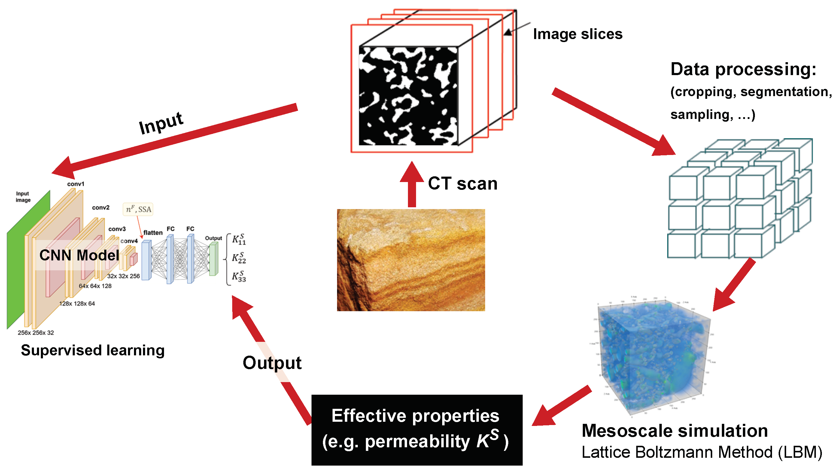
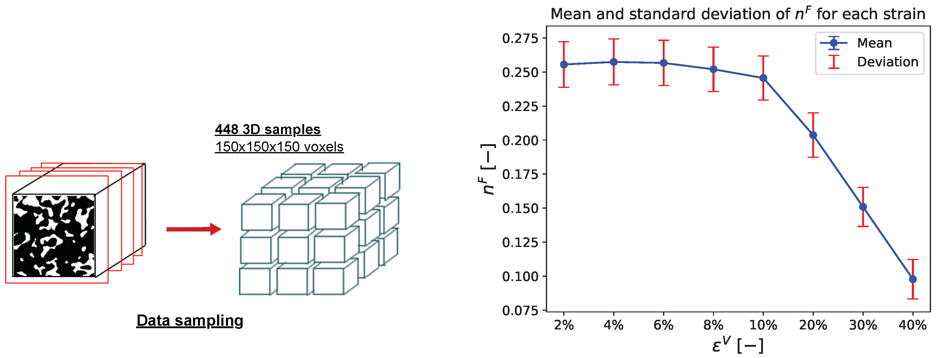
3. Database Generation

The database utilized in this study is derived from μ -CT images of Bentheim sandstone, accessible via the Digital Rock Portal [51] and hold a resolution of δ x 1 = δ x 2 = δ x 3 = 8.96 µm per pixel. These images are obtained at various deformation states, which correspond to volumetric strains ε V { 2 % , 4 % , 6 % , 8 % , 10 % , 20 % , 30 % , 40 % } . Each deformation state comprises eight samples, each consisting of 500–700 slices of 700 × 700 pixels.

3.1. Image Processing

In database preparation for the training, the raw CT images of the eight three-dimensional samples of 700 × 700 × 700 voxels undergo binarization and sampling. This process results in a sufficient database size of 448 three-dimensional (3D) samples. With this, each of the downscaled 3D samples has a size of 150 × 150 × 150 voxels to ensure manageable data size while preserving essential microstructural features. This treatment is consistent with the work of Hong and Liu [27]. An illustration of the data sampling to obtain 448 3D samples is presented in Figure 2, left.
Moreover, the binarization step is performed using thresholding to convert grayscale CT images into binary images, where the pore space and the solid matrix are distinguished. This allows the porosity ( n F ) of the material to be estimated for each strain level, showing the deformation dependency, as illustrated in Figure 2, right. Based on these binary images, the specific surface area (SSA), which is the ratio of the total surface area of the material per unit volume, can also be computed with the help of a Matlab code published by Degruyter et al. [52]. In addition, these binary images serve as the basis for simulations performed in Palabos [53], an open-source framework for lattice Boltzmann simulations.

3.2. Lbm for Single-Phase Fluid Flow

In this study, we employ lattice Boltzmann method (LBM) simulations to calculate the average fluid velocity within each 3D sample under an applied pressure gradient. This allows for the inverse calculation of the intrinsic permeability tensor using the Darcy flow equation presented in (15) with v S = 0 . Abstract introduction to the LBM in the context of single fluid flow is given below, while more details and references can be found in [33,36,54].
The LBM uses a mesh-based approach to solve the Boltzmann equation [55]. It starts by defining the velocity distribution function f ( x , ξ , t ) , which represents the probability of finding a fluid particle at a specific position x and time t with a certain discrete velocity ξ . The Boltzmann equation then describes how f ( x , ξ , t ) evolves over space and time. The evolution of f ( x , ξ , t ) , associated with the exchange of momentum and energy amongst these particles, occurs through two key processes—streaming and collision—viz.,
d f d t | streaming = d f d t | collision with f t + ξ · f x streaming operator = f t + v · f x Ω ( f ) . collision operator
As described in Krüger et al. [56] and He and Luo [57], the distribution function f ( x , ξ , t ) is linked to macroscopic variables such as fluid density ρ F R and fluid velocity v F through its moments. This connection is established using the following integrals:
ρ F R ( x , t ) ρ l ( x , t ) = f ( x , ξ , t ) d ξ and v F ( x , t ) u l ( x , t ) = 1 ρ l ξ f ( x , ξ , t ) d ξ .
For the spatial discretization in 3D, a fluid particle is restricted to stream in 19 possible directions, known as D3Q19. These directions are defined as follows:
e i = ( 0 , 0 , 0 ) i = 0 ( ± 1 , 0 , 0 ) , ( 0 , ± 1 , 0 ) , ( 0 , 0 , ± 1 ) i = 1 , 2 , , 6 ( ± 1 , ± 1 , 0 ) , ( ± 1 , 0 , ± 1 ) , ( 0 , ± 1 , ± 1 ) i = 7 , 8 , , 18 ,
where e i is the direction of the velocity vectors ξ i = c e i given in terms of c as the ratio of the distance between the nodes Δ x to the time-step size Δ t . Regarding the collision operator Ω ( f ) in (17), the Bhatnagar–Gross–Krook (BGK) [58] model is used since it is easy to implement and has been widely used in LBM fluid flow simulation [59]. In particular, the BGK collision operator Ω BGK is expressed as
Ω BGK = f i f i e q τ with τ : = 1 2 + ν l c s 2 .
Herein, the relaxation time τ depends on the lattice fluid viscosity ν l and lattice speed of sound c s = 1 / 3 . The BGK model facilitates the relaxation of the distribution functions f i toward equilibrium distributions f i e q at a collision frequency τ 1 . The formulation of f i e q is expressed as follows
f i e q = w i ρ l 1 + e i · u l c s 2 + ( e i · u l ) 2 2 c s 4 ( u l · u l ) 2 2 c s 2 ,
where w i presents the lattice weights, i.e.,
w i = 1 / 3 i = 0 1 / 18 i = 1 , 2 , , 6 1 / 36 i = 7 , 8 , , 18 .
The distribution functions are updated through the following equation:
f i ( x + ξ i Δ t , t + Δ t ) f i ( x , t )     streaming =   Ω BGK collision .
For the boundary conditions (BCs), the Zou-He [60] bounce-back boundary dynamics are used. For a more detailed explanation of the LBM approach for single-phase fluid flow, refer to [33].

3.3. Intrinsic Permeability Computation
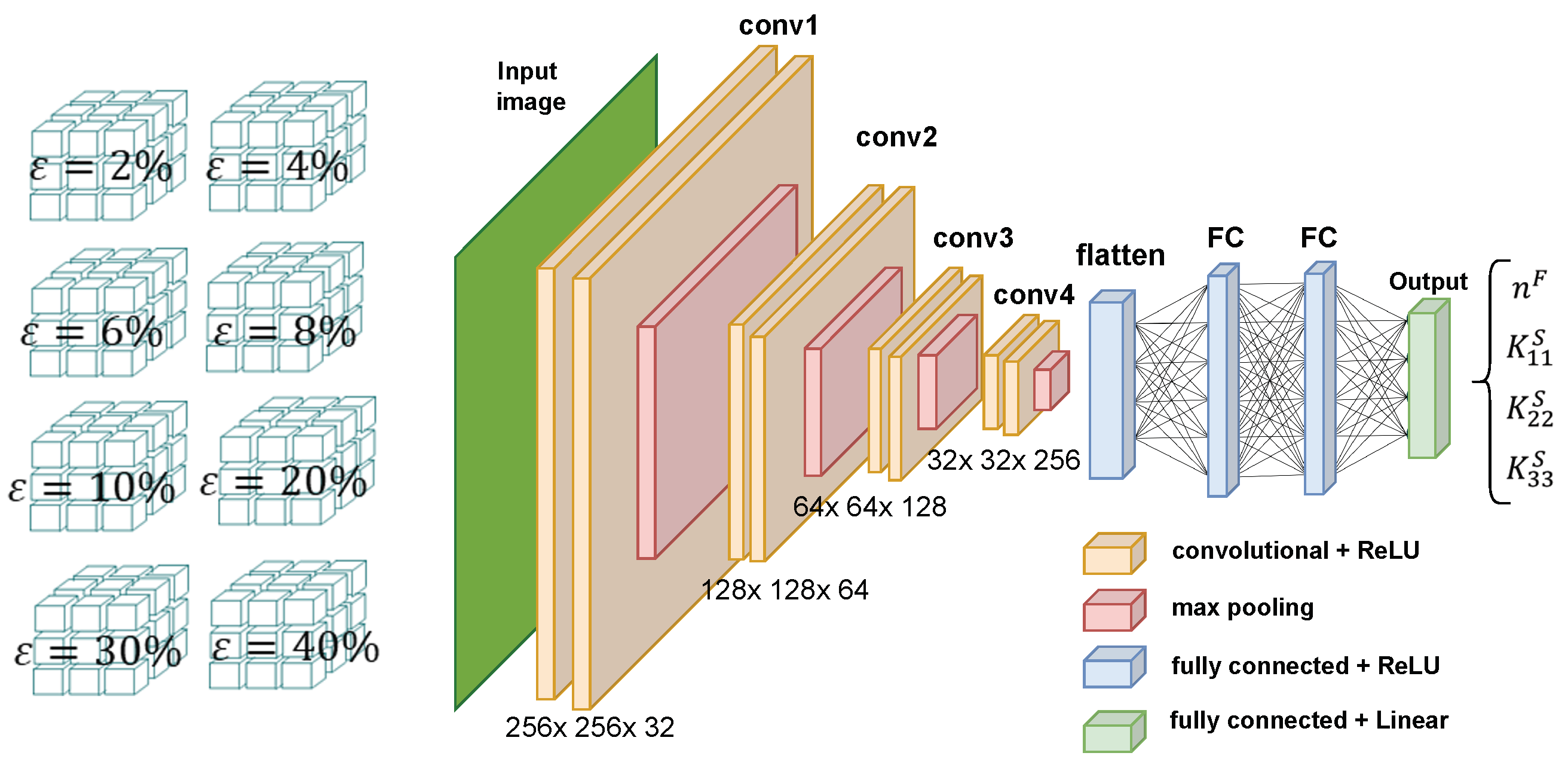
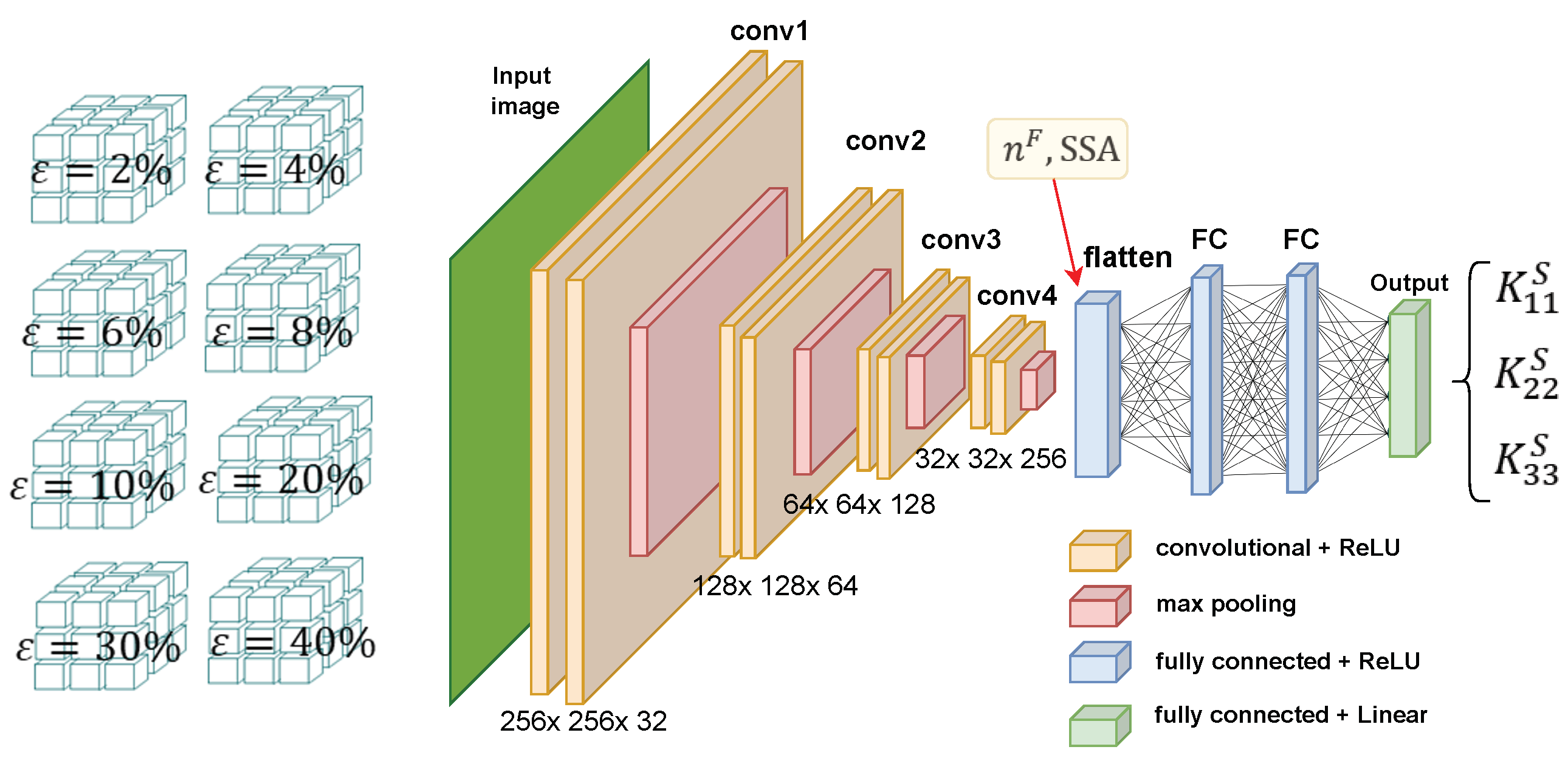
The proposed CNN model in this work uses CT images of sandstone as input and outputs the components of the permeability tensor. To consider the intrinsic permeability components in the database, 3D samples of Bentheim sandstone at varying levels of deformation are input into the single-phase LBM solver described in Section 3.2. The primary goal of the LBM simulation is to calculate the average lattice fluid velocity for each prescribed pressure gradient applied across the porous domain along the hydrodynamic axes x 1 , x 2 and x 3 , i.e., p 1 , p 2 and p 3 , respectively. The simulation results are used to determine the lattice intrinsic permeability tensor K l S in lattice units [l.u.]. This is done under the assumption that the permeability tensor is symmetric and positive definite [61]. As proposed by Kuhn et al. [61], two fluid flow simulations for each direction with different boundary conditions are to be carried out: one with no-slip boundary conditions and another with natural slip boundary conditions on surfaces parallel to the fluid flow direction (see Figure 3, left, for illustration). The rationale behind this is that the average velocity computed in the pressure direction is lower with no-slip boundary conditions compared to that with natural slip boundary conditions. The difference between these velocities indicates additional fluid flow in the direction orthogonal to the pressure gradient. The average velocities for the no-slip boundary conditions are then used to compute the diagonal components of the permeability tensor using a Darcy filter law:
( K l S ) i i = ν l ( u l ) i , avg i p l l . u . , with i = 1 , 2 , 3 .
In this, the lattice pressure gradient, presented by i p l = p l / x i is induced between two opposing surfaces perpendicular to the flow direction to calculate the average lattice fluid velocity ( u l ) i , avg . As for the latter, the unknown off-diagonal elements of the permeability tensor are computed using the average velocity with natural slip boundary conditions following [61] as
2 p l 3 p l 0 1 p l 0 3 p l 0 1 p l 2 p l ( K l S ) 12 ( K l S ) 13 ( K l S ) 23 = ν l ( u l ) 1 , avg ( K l S ) 11 1 p l ν l ( u l ) 2 , avg ( K l S ) 22 2 p l ν l ( u l ) 3 , avg ( K l S ) 33 3 p l .
The off-diagonal components we computed for Bentheim sandstone are much smaller than the diagonal components. Thus, we neglect them for simplicity from the ML model. In particular, the symmetric permeability tensor and its simplified diagonal form are expressed as follows:
K l S = ( K l S ) 11 ( K l S ) 12 ( K l S ) 13 ( K l S ) 21 ( K l S ) 22 ( K l S ) 23 ( K l S ) 31 ( K l S ) 32 ( K l S ) 33 ( e ¯ i e ¯ j ) ( K l S ) 11 0 0 0 ( K l S ) 22 0 0 0 ( K l S ) 33 ( e ¯ i e ¯ j ) .
Here, e ¯ i , e ¯ j represent the cartesian basis vectors with i , j { 1 , 2 , 3 } and ⊗ is the dyadic product (tensor product). In this connection, Figure 3, right, shows the mean and standard deviation of the diagonal intrinsic permeability components ( K l S ) 11 , ( K l S ) 22 , ( K l S ) 33 for each strain level ε V , showing the deformation dependency and anisotropy in the flow.
The macroscopic intrinsic permeability tensor is derived from the lattice permeability tensor as follows
K i j S = ( K l S ) i j ( δ x i δ x j ) in m 2 ,
where δ x i and δ x j characterize the spatial resolution of the μ -CT images in the i and j directions, respectively.
For simplicity, we will refer to the permeability tensor as ( K S ) , regardless of whether it is in [l.u.] or [ m 2 ], as this is only a unit change and does not affect the basic idea of the paper or the machine learning algorithms.

4. Model (1): [ K S n F ] -CNN Model

Convolutional neural networks (CNNs), as a class of deep learning artificial neural networks (ANN), are widely used in applications such as image classification, object detection, and text recognition. They mostly require data that have a grid-like nature, such as images or time series data (see, for example, [28,42,43,62,63,64,65] for reviews and applications). The CNN is considered as a sort of feed-forward NN (FFNN) approach with weight-sharing properties achieved through convolutional and pooling (subsampling) layers. In this work, the CNN models are implemented using Python 3.11.7, utilizing the deep learning open-source code Keras [66] with TensorFlow 2.15.0 [67] as the backend engine. The implementation and training processes are conducted in a Jupyter Notebook v.7.0.6 within an Anaconda environment. The training is performed on a NVIDIA H100 GPU with 80 GB of memory (NVIDIA, Santa Clara, CA, USA).
The following discussion presents a brief explanation of the proposed CNN model architecture, which considers μ -CT images of Bentheim sandstone as input to predict the associated permeability components. Additionally, porosity is included as part of the output, enabling the model to consider the deformed state of the material. The discussion will also cover the model’s training process and its performance on unseen data.

4.1. CNN Model Architecture and Hyperparameters

The CNN model comprises several key components, which are described as follows:
  • Convolution Operation: This step involves the application of a 2D filter (also known as a kernel or feature detector) to the input data, resulting in the generation of a feature map. This process highlights important features within the CT images by detecting patterns and edges that are crucial for permeability and porosity predictions.
  • Pooling Operation: After the convolution operation, a pooling layer is applied to the feature map. This process aims to down-sample the feature map by calculating, for instance, their maximum or average values and sending only the significant features to the next CNN layer.
  • Multi-Layer Perceptron (MLP): The MLP consists of fully connected (dense) layers that take the pooled feature map as input and produce a 1D feature vector as output.
The architecture of the proposed CNN model is illustrated in Figure 4 and is in line with the model presented in [42].
The following details are associated with the underlying model:
  • Data preparation:
    The image-related input data are transposed and reshaped to ensure compatibility with the 3D CNN model architecture.
    Before splitting into training, validation, and test subsets, data indices are shuffled to randomize the samples.
    After Splitting, the output data ( n F and K k k S ) are scaled using the MinMaxScaler, class of the sklearn.preprocessing toolkit [68], to normalize the values between 0 and 1, which is essential for stabilizing the training process.
  • Model architecture:
    The CNN model features four convolutional blocks, each comprising two 3D convolutional layers with increasing filter sizes (32, 64, 128, 256) and a kernel size progressively increasing from 3 × 3 × 3 to 7 × 7 × 7.
    Each convolutional layer employs ReLU activation and same padding to maintain spatial dimensions.
    Following each convolutional block, a MaxPooling3D layer with a pool size of 2 × 2 × 2 is incorporated to down-sample the spatial dimensions, reducing computational load and mitigating overfitting.
  • Fully-connected (dense) layers:
    Post convolutional and pooling operations, a Flatten layer transforms the 3D feature maps into a 1D feature vector.
    This 1D vector is then fed into a series of fully connected (Dense) layers, configured with 64 and 32 units respectively, both employing ReLU activation and L 2 regularization to prevent overfitting.
    The final Dense layer contains four units (related to n F and K k k S with k = 1 , 2 , 3 ) with a “linear” activation function, suitable for regression tasks.
  • Loss Function and Optimization:
    The model is compiled using the mean squared error (MSE) loss function, i.e.,
    D MSE = 1 n i = 1 n n i F , p n i F , t 2 + K k k , i S , p K k k , i S , t 2 ,
    where n is the number of output data points and k = 1 , 2 , 3 .
    Optimization is managed by the Adam optimizer, configured with a learning rate of 0.00001 .
  • Training and Callbacks:
    The training process spans up to 500 epochs, i.e., 500 complete passes through the entire training dataset, with a batch size of 16, comprising validation data to monitor performance.
    Callback mechanisms such as ReduceLROnPlateau, ModelCheckpoint, and EarlyStopping are implemented.

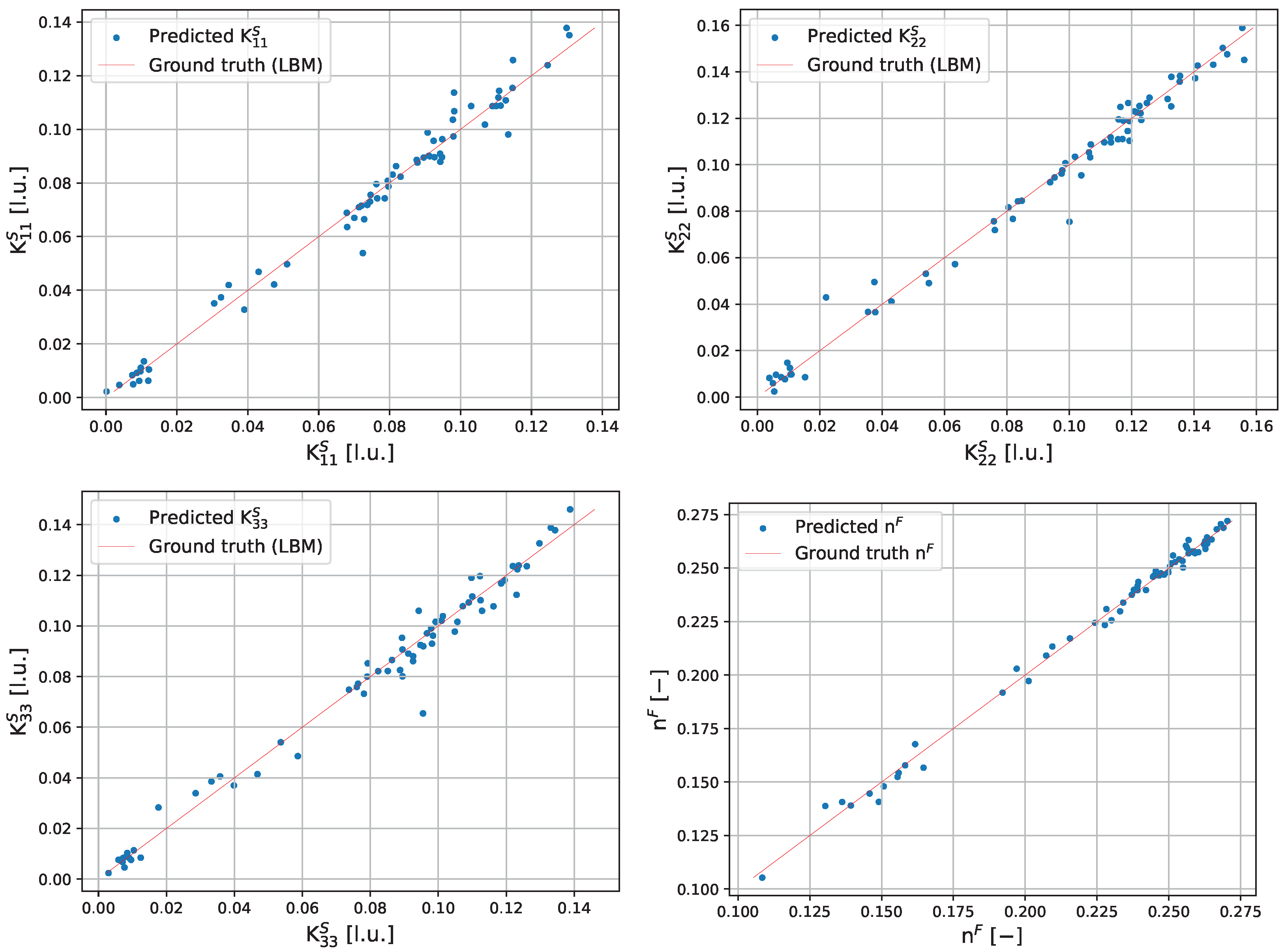
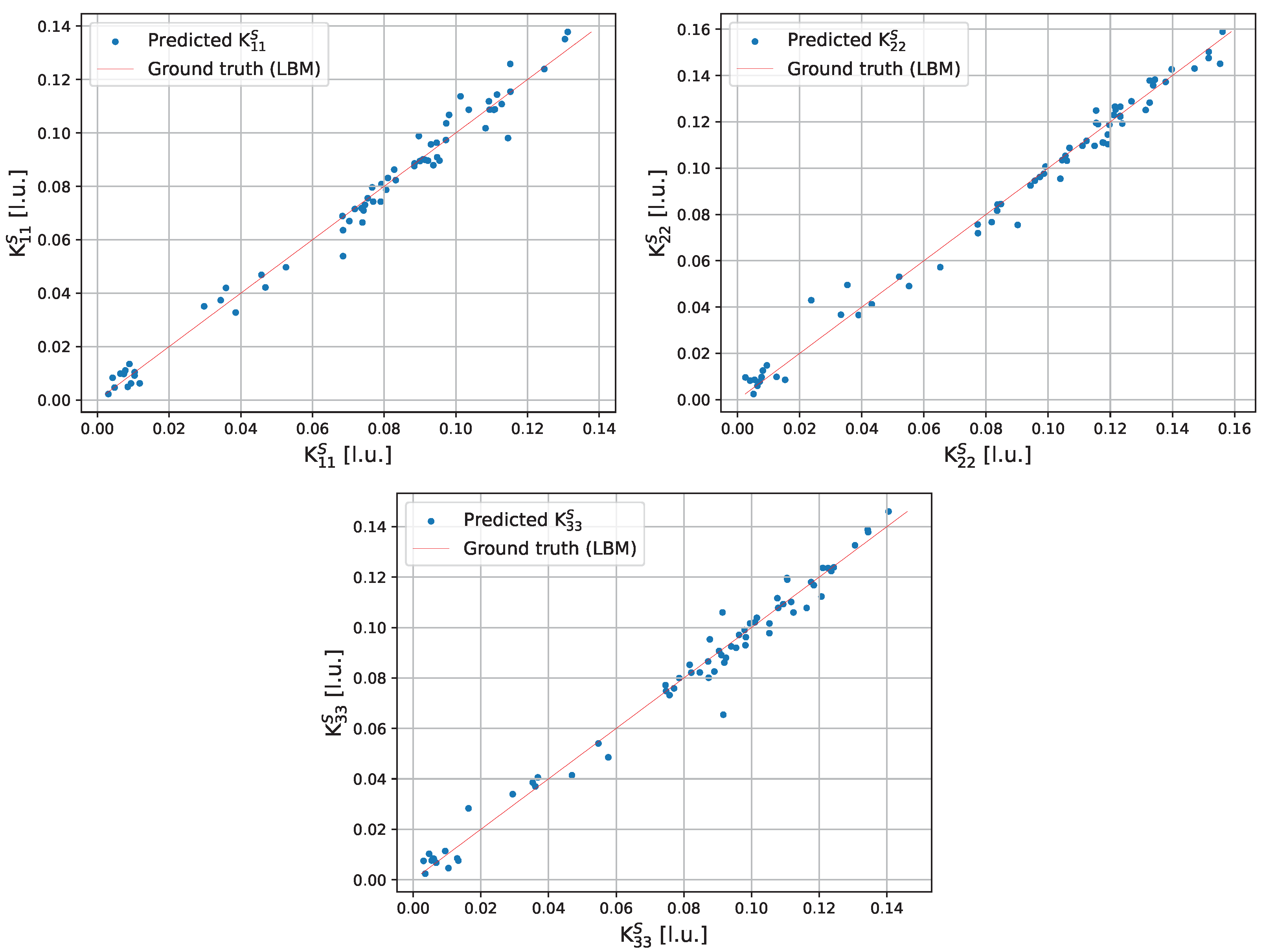
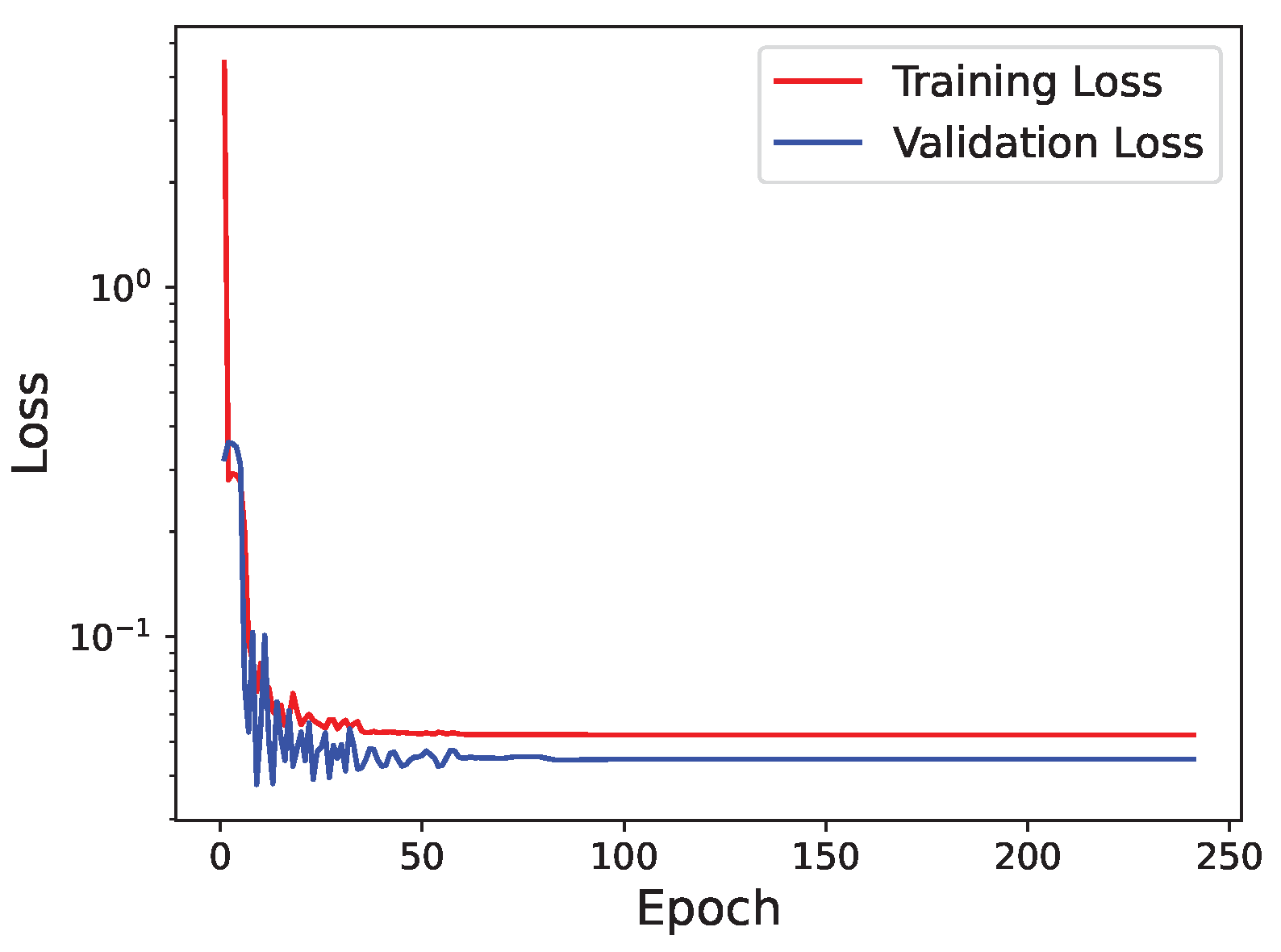
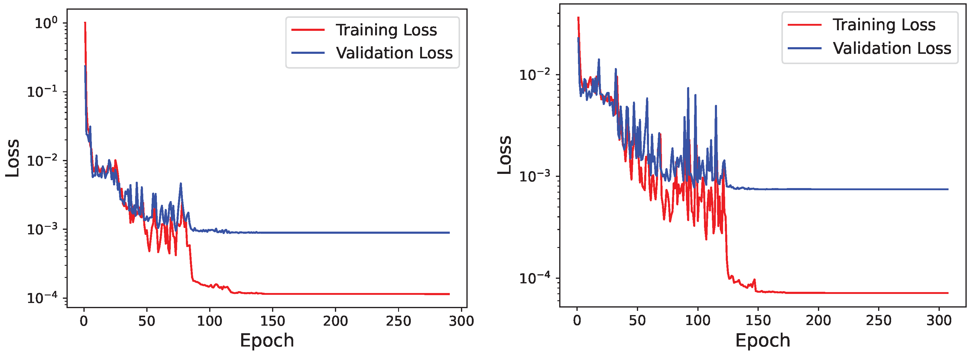
4.2. Training and Testing of Model (1)

The training process is monitored by evaluating both the training and validation losses over epochs, with the corresponding curves shown in Figure 5. Initially, both losses decrease rapidly, indicating that the model is learning effectively. As training continues, the training loss continues to decrease while the validation loss stabilizes, indicating some degree of overfitting. Despite tuning various hyperparameters, this issue could not be entirely eliminated. However, the validation loss remains stable at approximately 10 3 , which is within an acceptable range for permeability prediction as tested on unseen data. Since further training beyond 100 epochs does not improve generalization, but increases overfitting, we select Early Stopping at this point. Thus, the model at 100 epochs is used for testing, ensuring a balance between accuracy and generalization.
The scatter plots in Figure 6, which compare the predicted values to the ground truth values for the output variables n F and K k k S (for k = 1 , 2 , 3 ), further demonstrate the ability of the model to accurately predict the intrinsic permeability values and the corresponding porosity.
The model’s performance can quantitatively be assessed using the R 2 score, which is typically between 0 and 1 and calculated using the following formula:
R 2 = 1 i = 1 n ( y i h i ) 2 i = 1 n ( y i y ¯ ) 2 with y i : True value for the i - th data point , h i : Predicted value for the i - th data point , y ¯ : Mean of the true values , n : Number of data points .
The R 2 score achieved in this model is ≈0.985, demonstrating a high level of accuracy in predicting the output variables based on unseen data.

5. Model (2): Informed K S -CNN Model

Following the study of Wu et al. [26] to improve the accuracy of the CNN model, in this section, we test an alternative structure to our [ K S n F ] -CNN model presented in Section 4. In the modified structure, physical parameters, i.e., the porosity ( n F ) and the specific surface area (SSA), are incorporated directly into the network architecture instead of having n F in the loss function. This results in a kind of physical parameter-informed CNN, which we call “Informed K S -CNN model”. The modified structure of the CNN model is illustrated in Figure 7.
Specifically, an additional input branch (parallel branch) is added to the network to include n F and SSA, which are passed through a dense layer with 16 units and ReLU activation. Thus, the output of the Flatten layer (main branch) and the added parallel branch are concatenated to combine the information from both sources. Specifically, the concatenation layer merges the 1D feature vector from the image data and the supplementary features ( n F and SSA), allowing the model to exploit both image-based and additional data. As n F is no longer part of the output data, a modified MSE loss function needs to be considered, which is expressed as
D MSE = 1 n i = 1 n K k k , i S , p K k k , i S , t 2 ,
where n is the number of output data points and k = 1 , 2 , 3 .
The training results of the “Informed K S -CNN model” are evaluated through the loss vs. epoch curves, as illustrated in Figure 8. These show an initial rapid learning trend. However, similar to [ K S n F ] -CNN model, the validation loss begins to diverge from the training loss, indicating overfitting. Therefore, the model’s state after approximately 100 epochs, corresponding to a loss value of around 10 3 , was considered optimal for further evaluation.
The scatter plots in Figure 9, which compare the predicted values to the LBM-based ground truth values for the output variables K k k S (for k = 1 , 2 , 3 ), further demonstrate the ability of the model to accurately predict the intrinsic permeability values.
The performance of the “Informed K S -CNN model” is quantitatively assessed using the R 2 score. The model achieved an R 2 -score of 0.983, which indicates a high level of accuracy. Although the structure of Model (2) is more complicated than that of Model (1), its R 2 score is very close to that of Model (1). Thus, there is no significant advantage to using Model (2) over Model (1) in this particular model with the considered dataset. Based on this, further research on other datasets is needed to explore the potential benefits of integrating additional physical parameters into neural network architectures.

6. Model (3): Enriched [ K S n F ] -CNN Model

As an alternative to the approach in Section 5, we explore enhancing the CNN model’s performance and generalization through data augmentation, which increases the size and diversity of the training dataset. This improvement follows two key steps: (1) training an initial model on synthetic data to capture general patterns; and (2) applying transfer learning, where the pre-trained model is fine-tuned on the original dataset to refine its performance.
In this work, we utilize open-access synthetic data, published by Nguyen et al. [30], to enhance our CNN model’s predictions of permeability and porosity. The data were generated using generative adversarial networks (GANs), coupled with a pore network model (PNM) to produce visually and physically realistic 3D microstructures of Bentheim sandstone. Specifically, GANs are ML algorithms that were originally created in the realm of computer vision to produce synthetic images. GANs comprise a pair of neural networks (NNs), i.e., a generator and a discriminator. These NNs are trained concurrently in a game theory-inspired framework to generate synthetic datasets that resemble the source datasets (see, e.g., Goodfellow et al. [69]). On the other hand, pore network models (PNMs) are simplified representations of porous media that focus on the structure and connectivity of the pores and throats within the material [70]. PNMs are used to simulate fluid flow and transport properties in porous materials in a simplified way compared to the LBM. In [30], GANs are coupled with the PNMs using reinforcement learning (RL) to efficiently generate synthetic but realistic 3D images of porous media by incorporating physical constraints and properties derived from the PNMs. This GAN-PNM coupling approach ensures that the generated synthetic 3D images are not only visually realistic but also physically consistent with the characteristics of real porous media.
Focusing on Bentheim sandstone, Figure 10 illustrates the comparison between the ground truth and the generated microstructures, which exhibit controlled properties such as porosity, permeability, and specific surface area [30].

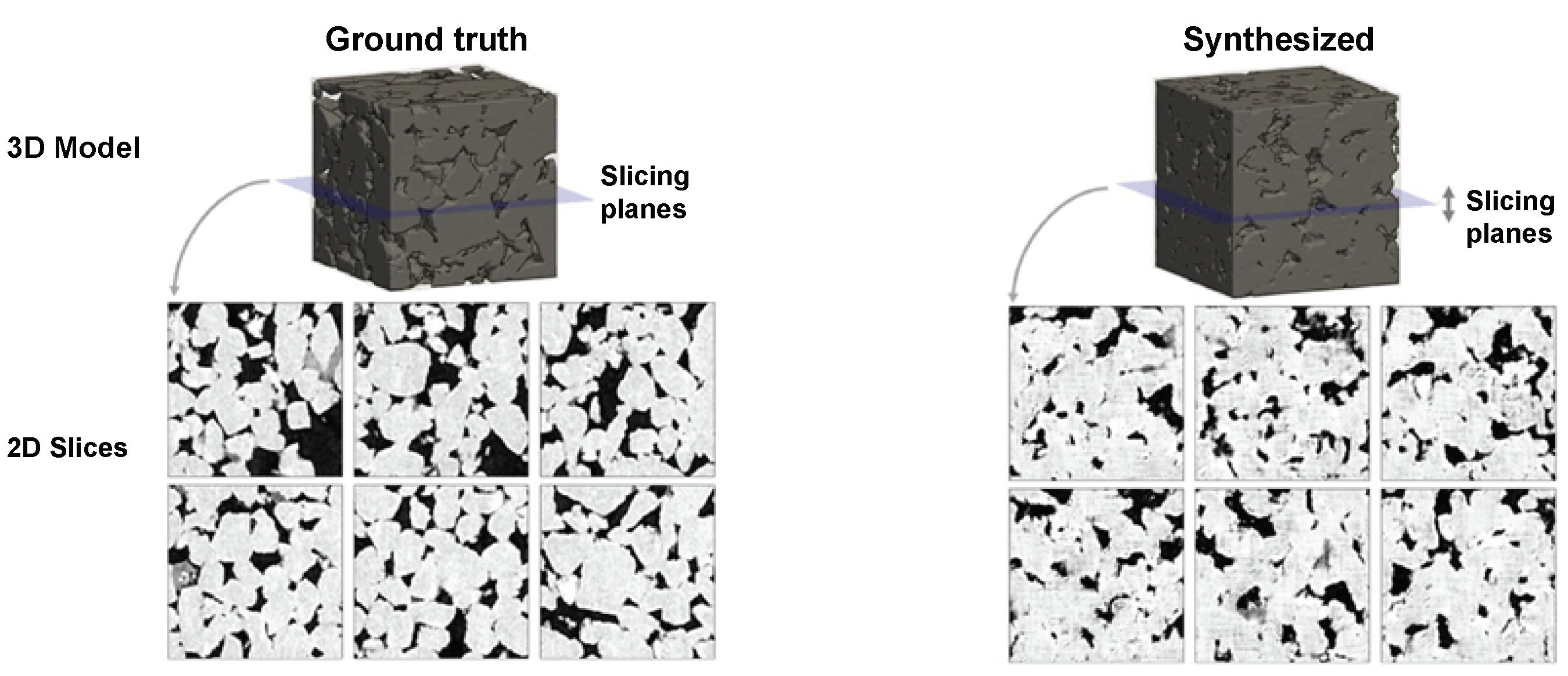
6.1. Training with the Synthetic Data

The open-access dataset we use for later processing comprises 10 3D volumes, each with dimensions of 216 × 216 × 128 voxels. During the dataset preparation for training, the gray-scaled synthetic microstructures are first binarized. The binarization threshold is selected to ensure that the resulting porosity matches that of the ground truth. Subsequently, the dataset is sampled, producing a final database consisting of 80 3D samples, each measuring 108 × 108 × 108 voxels. Following this, LBM simulations as explained in Section 3.2 are applied to each of the 3D volumes. To simplify this case of study, uni-directional flow is considered so that the permeability in the flow direction is computed, i.e., K 11 S . Thus, the loss function of this model is expressed as
D MSE = 1 n i = 1 n n i F , p n i F , t 2 + K 11 , i S , p K 11 , i S , t 2 ,
where n is the number of output data points.
The training process is carried out using the same model architecture and hyperparameters discussed in Section 4.1. The training is monitored by evaluating both the training and validation losses over epochs, with the corresponding curves shown in Figure 11.
Although the database is relatively small, both losses decrease rapidly, indicating that the model is learning effectively. As training continues, the training loss stabilizes at a slightly higher value compared to the validation loss, suggesting that the model is encountering some degree of underfitting. However, both values of the loss function are close to 5 × 10 2 . The weights and biases of the trained model are stored in a ∗.hdf5 file, which is then used for training on the original data within the context of transfer learning.

6.2. Transfer Learning Effect on the Model Learning

Transfer learning in our CNN model leverages the pre-trained model’s knowledge (weights and biases) from Section 6.1 to enhance learning efficiency and performance on the real dataset. This dataset consists of 448 3D volumes, each with dimensions of 108 × 108 × 108 voxels. Uni-directional flow simulations using the LBM are then conducted to generate the database, which includes permeability and porosity as outputs, as detailed in Section 3. The CNN model architecture and hyperparameters applied are identical to those described in Section 4.1, and the loss function is defined by Equation (31).
In this study, we compare two models: one without transfer learning (random initial weights) and one with transfer learning (initial weights from the pre-trained model on synthetic data). The results, illustrated in Figure 12, demonstrate that the model with transfer learning exhibits faster learning compared to the model without transfer learning. Notably, the initial loss value is around 1 for the model without transfer learning, while it is approximately 0.03 for the model with transfer learning. After sufficient epochs (around 300), the final values of the loss functions for both models are similar.
In summary, transfer learning significantly enhances the learning efficiency of the CNN model when applied to the original dataset. The pre-trained weights and biases facilitate quicker convergence, thereby reducing the computational resources and time required to achieve optimal performance. Thus, we conclude that the pre-trained weights and biases facilitate faster convergence and help reduce the computational resources and time required to achieve a well-trained model. To demonstrate the importance and effectiveness of this approach, further testing is needed, especially with smaller real datasets. In such cases, the generation of synthetic data and transfer learning could be crucial for the development of a well-trained ML model with high predictive power.

7. Discussion of the Approaches

After presenting the three models for permeability prediction in porous media, i.e., Model (1): [ K S n F ] -CNN, Model (2): Informed K S -CNN, and Model (3): Enriched [ K S n F ] -CNN model, this section presents a brief comparative discussion of these models. The first two models, Model (1) and Model (2), are directly comparable, as they consider exactly the same 3D samples of 150 × 150 × 150 voxels each. Model (3), however, considers 3D samples of 108 × 108 × 108 voxels each, as we need to ensure compatibility with the available synthetic data. Table 1 presents an overview and a comparison of the three CNN models.
While Model (1) offers simplicity and efficiency with high accuracy, Model (2) incorporates additional physical parameters but does not significantly improve performance. Model (3) leverages transfer learning, enhancing generalization but increasing computational cost due to the initial training on the synthetic data. For the data considered in this study, Model (1) remains a practical choice for efficiency.

8. Conclusions and Future Aspects

In this work, we have demonstrated the ability of different CNN models to accurately predict the anisotropic intrinsic permeability tensor together with the porosity at different deformation states. The inputs of this CNN model are real CT images related to Bentheim sandstone. The predicted parameters (outputs) can be directly integrated into a macroscopic TPM framework to describe both linear and non-linear flow through porous media, where different flow models have been discussed. Three CNN models are presented in this study: (1) an initial model that includes the permeability components and porosity in the definition of the loss function; (2) an informed CNN model that incorporates physical parameters directly into the model architecture; and (3) an enriched CNN model with transfer learning, where learning starts with synthetic data and the pre-trained model is fine-tuned on the original dataset. The initial CNN model showed high accuracy, while the informed CNN model did not significantly outperform the simpler initial model on the given dataset. However, data augmentation with synthetic data and the application of transfer learning proved effective in improving learning efficiency.
Future research will focus on several promising areas to further improve and extend current models. This includes exploring the potential of using CNN models for the inverse design of porous metamaterials with tailored hydro-mechanical properties, such as stiffness and permeability, which can be fabricated by additive manufacturing. Another future approach is physics-enhanced multiscale modeling, where physics-based constraints and principles are integrated into the multiscale modeling framework. This approach could potentially allow for the use of smaller datasets, improving the efficiency and feasibility of training accurate models without compromising performance. While the proposed model effectively predicts anisotropic permeability, future studies could test its application to fractured porous media, where anisotropic flow dominates. Regarding the model’s potential applicability to porous media beyond Bentheim sandstone, several approaches can be explored. For instance, transfer learning can be utilized, where the initial training is conducted on Bentheim sandstone and then fine-tuned for other materials. Additionally, physics-constrained models could be incorporated, as they are known to enhance accuracy while requiring fewer data. However, these approaches would necessitate further validation in future works to ensure robustness and reliability.

Author Contributions

Conceptualization, Y.H.; Methodology, Y.H., F.A. and W.E.; Software, Y.H.; Resources, F.A.; Writing—original draft, Y.H. and F.A.; Supervision, W.E. All authors have read and agreed to the published version of the manuscript.

Funding

Y. Heider would like to gratefully thank the German Research Foundation (DFG) for its funding support through the project “Multi-field continuum modeling of two-fluid-filled porous media fracture augmented by microscale-based machine-learning material laws”, grant number 458375627. F. Aldakheel gratefully acknowledges funding support for this research by the “German Research Foundation” (DFG) through the SFB/TRR-298-SIIRI—Project-ID 426335750.

Institutional Review Board Statement

Not applicable.

Informed Consent Statement

Not applicable.

Data Availability Statement

Exemplary source codes are available as open access for interested readers at https://doi.org/10.25835/xrii0m6f (accessed on 1 January 2025).

Conflicts of Interest

The authors declare no conflicts of interest.

Abbreviations

The following abbreviations are used in this manuscript:
ANNArtificial neural networks
CNNConvolutional neural networks
CTComputed tomography
RVERepresentative volume elements
LBMLattice Boltzmann method
TPMTheory of porous media
SSASpecific surface area
MLMachine learning
BGKBhatnagar–Gross–Krook
DNNDeep neural networks
GANGenerative adversarial networks
PNMPore network model
RNNRecurrent neural networks
FFNNFeed-forward neural networks

References

  1. Ehlers, W. Darcy, Forchheimer, Brinkman and Richards: Classical hydromechanical equations and their significance in the light of the TPM. Arch. Appl. Mech. 2022, 92, 619–639. [Google Scholar] [CrossRef]
  2. Ehlers, W.; Graf, T.; Ammann, M. Deformation and localization analysis of partially saturated soil. Comput. Methods Appl. Mech. Eng. 2004, 193, 2885–2910. [Google Scholar] [CrossRef]
  3. Mosthaf, K.; Baber, K.; Flemisch, B.; Helmig, R.; Leijnse, A.; Rybak, I.; Wohlmuth, B. A coupling concept for two-phase compositional porous-medium and single-phase compositional free flow. Water Resour. Res. 2011, 47, W10522. [Google Scholar] [CrossRef]
  4. Markert, B.; Heider, Y.; Ehlers, W. Comparison of monolithic and splitting solution schemes for dynamic porous media problem. Int. J. Numer. Meth. Eng. 2010, 82, 1341–1383. [Google Scholar] [CrossRef]
  5. Markert, B. A survey of selected coupled multifield problems in computational mechanics. J. Coupled. Syst. Multiscale Dyn. 2013, 27, 22–48. [Google Scholar] [CrossRef]
  6. Ehlers, W.; Wagner, A. Modelling and simulation methods applied to coupled problems in porous-media mechanics. Arch. Appl. Mech. 2019, 89, 609–628. [Google Scholar] [CrossRef]
  7. Heider, Y. A review on phase-field modeling of hydraulic fracturing. Eng. Fract. Mech. 2021, 253, 107881. [Google Scholar] [CrossRef]
  8. Peters, S.; Heider, Y.; Markert, B. Numerical simulation of miscible multiphase flow and fluid–fluid interaction in deformable porous media. PAMM 2023, 23, e202300209. [Google Scholar] [CrossRef]
  9. Miehe, C.; Mauthe, S. Phase field modeling of fracture in multi-physics problems. Part III. Crack driving forces in hydro-poro-elasticity and hydraulic fracturing of fluid-saturated porous media. Comput. Methods Appl. Mech. Eng. 2016, 304, 619–655. [Google Scholar] [CrossRef]
  10. Gawin, D.; Pesavento, F.; Koniorczyk, M.; Schrefler, B.A. Poro-mechanical model of strain hysteresis due to cyclic water freezing in partially saturated porous media. Int. J. Solids Struct. 2020, 206, 322–339. [Google Scholar] [CrossRef]
  11. Wang, K.; Sun, W. An updated Lagrangian LBM–DEM–FEM coupling model for dual-permeability fissured porous media with embedded discontinuities. Comput. Methods Appl. Mech. Eng. 2019, 344, 276–305. [Google Scholar] [CrossRef]
  12. Choo, J.; Borja, R.I. Stabilized mixed finite elements for deformable porous media with double porosity. Comput. Methods Appl. Mech. Eng. 2015, 293, 131–154. [Google Scholar] [CrossRef]
  13. Jenny, P.; Lee, S.H.; Tchelepi, H.A. Adaptive multiscale finite-volume method for multiphase flow and transport in porous media. Multiscale Model. Simul. 2005, 3, 50–64. [Google Scholar] [CrossRef]
  14. Heider, Y.; Wang, K.; Sun, W. SO (3)-invariance of informed-graph-based deep neural network for anisotropic elastoplastic materials. Comput. Methods Appl. Mech. Eng. 2020, 363, 112875. [Google Scholar] [CrossRef]
  15. Heider, Y.; Sun, W. Objectivity and accuracy enhancement within ANN-based multiscale material modeling. PAMM 2023, 22, e202200203. [Google Scholar] [CrossRef]
  16. Fuchs, A.; Heider, Y.; Wang, K.; Sun, W.; Kaliske, M. DNN2: A hyper-parameter reinforcement learning game for self-design of neural network based elasto-plastic constitutive descriptions. Comput. Struct. 2021, 249, 106505. [Google Scholar] [CrossRef]
  17. Tragoudas, A.; Alloisio, M.; Elsayed, E.S.; Gasser, T.C.; Aldakheel, F. An enhanced deep learning approach for vascular wall fracture analysis. Arch. Appl. Mech. 2024, 94, 2519–2532. [Google Scholar] [CrossRef]
  18. Aldakheel, F.; Satari, R.; Wriggers, P. Feed-forward neural networks for failure mechanics problems. Appl. Sci. 2021, 11, 6483. [Google Scholar] [CrossRef]
  19. Linden, L.; Klein, D.K.; Kalina, K.A.; Brummund, J.; Weeger, O.; Kästner, M. Neural networks meet hyperelasticity: A guide to enforcing physics. J. Mech. Phys. Solids 2023, 179, 105363. [Google Scholar] [CrossRef]
  20. Wessels, H.; Böhm, C.; Aldakheel, F.; Hüpgen, M.; Haist, M.; Lohaus, L.; Wriggers, P. Computational Homogenization Using Convolutional Neural Networks. In Current Trends and Open Problems in Computational Mechanics; Aldakheel, F., Hudobivnik, B., Soleimani, M., Wessels, H., Weißenfels, C., Marino, M., Eds.; Springer International Publishing: Cham, Switzerland, 2022; pp. 569–579. [Google Scholar] [CrossRef]
  21. Jin, H.; Zhang, E.; Espinosa, H.D. Recent Advances and Applications of Machine Learning in Experimental Solid Mechanics: A Review. Appl. Mech. Rev. 2023, 75, 061001. [Google Scholar] [CrossRef]
  22. Wang, K.; Sun, W. A multiscale multi-permeability poroplasticity model linked by recursive homogenizations and deep learning. Comput. Methods Appl. Mech. Eng. 2018, 334, 337–380. [Google Scholar] [CrossRef]
  23. Heider, Y.; Suh, H.S.; Sun, W. An offline multi-scale unsaturated poromechanics model enabled by self-designed/self-improved neural networks. Int. J. Numer. Anal. Methods Geomech. 2021, 45, 1212–1237. [Google Scholar] [CrossRef]
  24. Cai, C.; Vlassis, N.; Magee, L.; Ma, R.; Xiong, Z.; Bahmani, B.; Wong, T.F.; Wang, Y.; Sun, W. Equivariant Geometric Learning for Digital Rock Physics: Estimating Formation Factor and Effective Permeability Tensors from Morse Graph. Int. J. Multiscale Comput. Eng. 2023, 21, 1–24. [Google Scholar] [CrossRef]
  25. Chaaban, M.; Heider, Y.; Sun, W.; Markert, B. A machine-learning supported multi-scale LBM-TPM model of unsaturated, anisotropic, and deformable porous materials. Int. J. Numer. Anal. Methods Geomech. 2024, 4, 889–910. [Google Scholar] [CrossRef]
  26. Wu, J.; Yin, X.; Xiao, H. Seeing permeability from images: Fast prediction with convolutional neural networks. Sci. Bull. 2018, 63, 1215–1222. [Google Scholar] [CrossRef] [PubMed]
  27. Hong, J.; Liu, J. Rapid estimation of permeability from digital rock using 3D convolutional neural network. Comput. Geosci. 2020, 24, 1523–1739. [Google Scholar] [CrossRef]
  28. Bishara, D.; Xie, Y.; Liu, W.K.; Li, S. A State-of-the-Art Review on Machine Learning-Based Multiscale Modeling, Simulation, Homogenization and Design of Materials. Arch. Comput. Methods Eng. 2023, 30, 191–222. [Google Scholar] [CrossRef]
  29. Herrmann, L.; Kollmannsberger, S. Deep learning in computational mechanics: A review. Comput. Mech. 2024, 74, 281–331. [Google Scholar] [CrossRef]
  30. Nguyen, P.C.H.; Vlassis, N.N.; Bahmani, B.; Sun, W.; Udaykumar, H.S.; Baek, S.S. Synthesizing controlled microstructures of porous media using generative adversarial networks and reinforcement learning. Sci. Rep. 2022, 12, 9034. [Google Scholar] [CrossRef] [PubMed]
  31. Ehlers, W. Foundations of multiphasic and porous materials. In Porous Media: Theory, Experiments and Numerical Applications; Ehlers, W., Bluhm, J., Eds.; Springer: Berlin/Heidelberg, Germany, 2002; pp. 3–86. [Google Scholar]
  32. Markert, B. A constitutive approach to 3-d nonlinear fluid flow through finite deformable porous continua. Transp. Porous Media 2007, 70, 427. [Google Scholar] [CrossRef]
  33. Chaaban, M.; Heider, Y.; Markert, B. Upscaling LBM-TPM simulation approach of Darcy and non-Darcy fluid flow in deformable, heterogeneous porous media. Int. J. Heat Fluid Flow 2020, 83, 108566. [Google Scholar] [CrossRef]
  34. Markert, B. Advances in Extended and Multifield Theories for Continua; Springer Science & Business Media: Berlin, Germany, 2011; Volume 59. [Google Scholar]
  35. De Marchi, N.; Xotta, G.; Ferronato, M.; Salomoni, V. An efficient multi-field dynamic model for 3D wave propagation in saturated anisotropic porous media. J. Comput. Phys. 2024, 510, 113082. [Google Scholar] [CrossRef]
  36. Chaaban, M.; Heider, Y.; Markert, B. A multiscale LBM–TPM–PFM approach for modeling of multiphase fluid flow in fractured porous media. Int. J. Numer. Anal. Methods Geomech. 2022, 46, 2698–2724. [Google Scholar] [CrossRef]
  37. Phu, N.T.; Navrath, U.; Heider, Y.; Carmai, J.; Markert, B. Investigating the impact of deformation on foam permeability through CT scans and the Lattice-Boltzmann method. PAMM 2024, 24, e202300154. [Google Scholar] [CrossRef]
  38. Zhang, X.; Huang, T.; Ge, Z.; Man, T.; Huppert, H.E. Infiltration characteristics of slurries in porous media based on the coupled Lattice-Boltzmann discrete element method. Comput. Geotech. 2025, 177, 106865. [Google Scholar] [CrossRef]
  39. Yang, G.; Xu, R.; Tian, Y.; Guo, S.; Wu, J.; Chu, X. Data-driven methods for flow and transport in porous media: A review. Int. J. Heat Mass Transf. 2024, 235, 126149. [Google Scholar] [CrossRef]
  40. Jiao, S.; Li, W.; Li, Z.; Gai, J.; Zou, L.; Su, Y. Hybrid physics-machine learning models for predicting rate of penetration in the Halahatang oil field, Tarim Basin. Sci. Rep. 2024, 14, 5957. [Google Scholar] [CrossRef]
  41. Chen, J.; Gildin, E.; Killough, J.E. Transfer Learning-Based Physics-Informed Convolutional Neural Network for Simulating Flow in Porous Media with Time-Varying Controls. Mathematics 2024, 12, 3281. [Google Scholar] [CrossRef]
  42. Aldakheel, F.; Soyarslan, C.; Palanisamy, H.S.; Elsayed, E.S. Machine learning aided multiscale magnetostatics. Mech. Mater. 2023, 184, 104726. [Google Scholar] [CrossRef]
  43. Aldakheel, F.; Elsayed, E.; Zohdi, T.; Wriggers, P. Efficient multiscale modeling of heterogeneous materials using deep neural networks. Comput. Mech. 2023, 72, 155–171. [Google Scholar] [CrossRef]
  44. Bowen, R.M. Theory of Mixtures. In Continuum Physics; Eringen, A.C., Ed.; Academic Press: New York, NY, USA, 1976; Volume III, pp. 1–127. [Google Scholar]
  45. Haupt, P. Foundation of Continuum Mechanics. In Continuum Mechanics in Environmental Sciences and Geophysics; Hutter, K., Ed.; CISM Courses and Lectures No. 337; Springer: Berlin/Heidelberg, Germany, 1993; pp. 1–77. [Google Scholar]
  46. Heider, Y.; Markert, B. A phase-field modeling approach of hydraulic fracture in saturated porous media. Mech. Res. Commun. 2017, 80, 38–46. [Google Scholar] [CrossRef]
  47. Bishop, A.W. The effective stress principle. Tek. Ukebl. 1959, 39, 859–863. [Google Scholar]
  48. de Boer, R.; Ehlers, W. The development of the concept of effective stresses. Acta Mech. 1990, 83, 77–92. [Google Scholar] [CrossRef]
  49. Ehlers, W. Effective Stresses in Multiphasic Porous Media: A thermodynamic investigation of a fully non-linear model with compressible and incompressible constituents. Geomech. Energy Environ. 2018, 15, 35–46. [Google Scholar] [CrossRef]
  50. Brinkman, H. A calculation of the viscous force exerted by a flowing fluid on a dense swarm of particles. Appl. Sci. Res. A 1949, 1, 27–34. [Google Scholar] [CrossRef]
  51. Moon, C.; Andrew, M. Bentheimer Networks. 2019. Available online: http://www.digitalrocksportal.org/projects/223 (accessed on 1 September 2024). [CrossRef]
  52. Degruyter, W.; Burgisser, A.; Bachmann, O.; Malaspinas, O. Synchrotron X-ray microtomography and lattice Boltzmann simulations of gas flow through volcanic pumices. Geosphere 2010, 6, 470–481. [Google Scholar] [CrossRef]
  53. Latt, J.; Malaspinas, O.; Kontaxakis, D.; Parmigiani, A.; Lagrava, D.; Brogi, F.; Belgacem, M.B.; Thorimbert, Y.; Leclaire, S.; Li, S.; et al. Palabos: Parallel Lattice Boltzmann Solver. Comput. Math. Appl. 2020, 81, 334–350. [Google Scholar] [CrossRef]
  54. Chaaban, M.; Heider, Y.; Markert, B. A multiscale study of the retention behavior and hydraulic anisotropy in deformable porous media. PAMM 2023, 23, e202200129. [Google Scholar] [CrossRef]
  55. Boltzmann, L. Lectures on Gas Theory; Brush, S.G., Translator; Originally Published as Vorlesungen über Gastheorie in 1896–1898; Dover Publications: New York, NY, USA, 1964. [Google Scholar]
  56. Krüger, T.; Kusumaatmaja, H.; Kuzmin, A.; Shardt, O.; Silva, G.; Viggen, E.M. The Lattice BOltzmann Method; Springer International Publishing: Cham, Switzerland, 2017; Volume 10, pp. 4–15. [Google Scholar]
  57. He, X.; Luo, L.S. Theory of the lattice Boltzmann method: From the Boltzmann equation to the lattice Boltzmann equation. Phys. Rev. E 1997, 56, 6811–6817. [Google Scholar] [CrossRef]
  58. Bhatnagar, P.L.; Gross, E.P.; Krook, M. A Model for Collision Processes in Gases. I. Small Amplitude Processes in Charged and Neutral One-Component Systems. Phys. Rev. 1954, 94, 511–525. [Google Scholar] [CrossRef]
  59. Wolf-Gladrow, D.A. Lattice-Gas Cellular Automata and Lattice Boltzmann Models: An Introduction; Springer: Berlin/Heidelberg, Germany, 2004. [Google Scholar]
  60. Zou, Q.; He, X. On pressure and velocity boundary conditions for the lattice Boltzmann BGK model. Phys. Fluids 1997, 9, 1591–1598. [Google Scholar] [CrossRef]
  61. Kuhn, M.R.; Sun, W.; Wang, Q. Stress-induced anisotropy in granular materials: Fabric, stiffness, and permeability. Acta Geotech. 2015, 10, 399–419. [Google Scholar] [CrossRef]
  62. Gu, J.; Wang, Z.; Kuen, J.; Ma, L.; Shahroudy, A.; Shuai, B.; Liu, T.; Wang, X.; Wang, G.; Cai, J.; et al. Recent advances in convolutional neural networks. Pattern Recognit. 2018, 77, 354–377. [Google Scholar] [CrossRef]
  63. Eidel, B. Deep CNNs as universal predictors of elasticity tensors in homogenization. Comput. Methods Appl. Mech. Eng. 2023, 403, 115741. [Google Scholar] [CrossRef]
  64. Dhillon, A.; Verma, G. Convolutional neural network: A review of models, methodologies and applications to object detection. Prog. Artif. Intell. 2020, 9, 85–112. [Google Scholar] [CrossRef]
  65. Tandale, S.; Stoffel, M. Recurrent and convolutional neural networks in structural dynamics: A modified attention steered encoder–decoder architecture versus LSTM versus GRU versus TCN topologies to predict the response of shock wave-loaded plates. Comput. Mech. 2023, 72, 765–786. [Google Scholar] [CrossRef]
  66. Chollet, F. Keras. 2015. Available online: https://github.com/fchollet/keras (accessed on 1 April 2024).
  67. Abadi, M.; Agarwal, A.; Barham, P.; Brevdo, E.; Chen, Z.; Citro, C.; Corrado, G.S.; Davis, A.; Dean, J.; Devin, M.; et al. Tensorflow: Large-scale machine learning on heterogeneous distributed systems. arXiv 2016, arXiv:1603.04467. [Google Scholar]
  68. Pedregosa, F.; Varoquaux, G.; Gramfort, A.; Michel, V.; Thirion, B.; Grisel, O.; Blondel, M.; Prettenhofer, P.; Weiss, R.; Dubourg, V.; et al. Scikit-learn: Machine learning in Python. J. Mach. Learn. Res. 2011, 12, 2825–2830. [Google Scholar]
  69. Goodfellow, I.; Pouget-Abadie, J.; Mirza, M.; Xu, B.; Warde-Farley, D.; Ozair, S.; Courville, A.; Bengio, Y. Generative adversarial networks. Commun. Acm 2020, 63, 139–144. [Google Scholar] [CrossRef]
  70. Gostick, J.; Aghighi, M.; Hinebaugh, J.; Tranter, T.; Hoeh, M.A.; Day, H.; Spellacy, B.; Sharqawy, M.H.; Bazylak, A.; Burns, L.; et al. OpenPNM: A pore network modeling package. Comput. Sci. Eng. 2016, 18, 60–74. [Google Scholar] [CrossRef]
Figure 1. Overview of the major steps of the 2D CNN model for predicting the effective properties of porous media (mainly permeability) based on CT images. This includes the input, the output, dataset preparation (cropping, segmentation, sampling), and model training.
Applsci 15 02589 g001
Figure 2. Illustration of data sampling in which 448 3D samples are generated (left). Mean and standard deviation of the porosity n F for each strain level ε V showing the deformation dependency, while the 448 samples are considered (right).
Applsci 15 02589 g002
Figure 3. Illustration of data generation using LBM with prescribed pressure difference and no-slip/natural slip BCs (left). Mean and standard deviation of the intrinsic permeability components K i i S for each strain level ε V , showing the deformation dependency and anisotropy (right).
Applsci 15 02589 g003
Figure 4. Architecture of the 3D CNN illustrating the flow of information from the input image through multiple convolutional layers, max pooling layers, and fully connected layers. The input image is a 3D volume with dimensions 256 × 256 × 32 , which passes through four convolutional layers (Conv1 to Conv4), each followed by max pooling to reduce spatial dimensions. After flattening, the feature maps are processed by two fully connected (FC) layers before generating the final output predictions ( n F , K 11 S , K 22 S , K 33 S ).
Applsci 15 02589 g004
Figure 5. Model (1): Training and validation loss function values over the number of weight updates (Epoch). The validation loss (blue curve) initially follows a similar trend to that of training loss (red curve) but starts to diverge after approximately 100 epochs, suggesting overfitting beyond this point.
Applsci 15 02589 g005
Figure 6. Model (1): CNN predictions vs. ground truth values of the intrinsic permeability components and porosity. The close alignment of the predicted values with the red line indicates a high prediction accuracy, confirming the model’s effectiveness in estimating permeability and porosity values.
Applsci 15 02589 g006
Figure 7. Illustration of the “Informed K S -CNN model” architecture (see Figure 4 for comparison). This illustration shows the information flow and the inclusion of the physical information ( n F and SSA) through an additional input branch.
Applsci 15 02589 g007
Figure 8. Model (2): Training and validation loss function values over the number of weight updates (Epoch). The validation loss (blue curve) initially follows a similar trend to that of training loss (red curve) but starts to diverge after approximately 100 epochs, suggesting overfitting beyond this point.
Applsci 15 02589 g008
Figure 9. Model (2): CNN predictions vs. ground truth values of the intrinsic permeability components. The close alignment of the predicted values with the red line indicates a high prediction accuracy, confirming the model’s effectiveness in estimating permeability and porosity values.
Applsci 15 02589 g009
Figure 10. 2D slices and 3D volume representations of real microstructures with those generated by GANs. The synthetic microstructures exhibit not only high visual fidelity, but also controlled properties such as porosity, permeability, and specific surface area (Source: Nguyen et al. [30]).
Applsci 15 02589 g010
Figure 11. Model (3): Training and validation loss function values over the number of weight updates (Epoch) with training on synthetic data. The validation loss (blue curve) initially follows a similar trend to that of training loss (red curve) but starts to diverge after some epochs, suggesting a slight underfitting.
Applsci 15 02589 g011
Figure 12. Model (3): Training and validation loss function values over the number of weight updates (Epoch) with no transfer learning (left) and with transfer learning (right). In both cases, the validation loss (blue curve) initially follows a similar trend to that of training loss (red curve) but starts to diverge after approximately 90 (right) and 100 (left) epochs, suggesting overfitting beyond this point.
Applsci 15 02589 g012
Table 1. Comparison of the three CNN models.
FeatureModel (1): [ K S n F ] -CNNModel (2): Informed K S -CNNModel (3): Enriched [ K S n F ] -CNN
Input μ -CT images μ -CT images μ -CT images
+ physical parameters ( n F , SSA)(Real & synthetic)
Output K S , n F K S K S , n F
Loss functionIncludes K S , n F Includes only K S Includes K S , n F
ComplexityModerateHigher (additional input branchHighest (pre-training
& complicated CNN architecture)& transfer learning)
TrainingSome overfitting (≈ 10 3 loss)Similar overfitting (≈ 10 3 loss)Similar overfitting (≈ 10 3 loss)
Final R 2 score≈0.985≈0.983Similar to Model (1) (≈0.985)
AdvantageSimple & effectiveIncorporates physical informationFaster training,
in the CNN architecturegood for small datasets
Disclaimer/Publisher’s Note: The statements, opinions and data contained in all publications are solely those of the individual author(s) and contributor(s) and not of MDPI and/or the editor(s). MDPI and/or the editor(s) disclaim responsibility for any injury to people or property resulting from any ideas, methods, instructions or products referred to in the content.

