Simulation and Experimental Research on Composite Diaphragm Hydraulic Force/Displacement Amplification Mechanism with Adjustable Initial Volume

Abstract

To improve the practicability of electro-mechanical converters in hydraulic systems, especially in control valves, a hydraulic force/displacement amplification mechanism was addressed. The amplification mechanism includes a rolling diaphragm (RD) and a corrugated diaphragm (CD), and the amplification function is achieved using the area difference between the RD and the CD. To investigate the amplification characteristics of the mechanism, the diaphragm forces were analyzed by finite element simulations, and the dynamic model of the system was established in Simulink, based on the force balance method. Furthermore, an amplification mechanism prototype was fabricated, and the static and dynamic experiments were carried out. Combining the simulation and experiment results, the accuracy of the proposed dynamic model was verified, and the amplification characteristics of the amplification mechanism were analyzed. When the RD displacement is less than 2 mm, the force amplification effect is not obvious. When the RD displacement exceeds 2 mm, the force amplification ratio (FAR) increases with the RD displacement and decreases with the CD displacement. The maximum FAR is 2.5 with a CD displacement of 0 and an RD displacement of 6 mm. The amplification mechanism and the used research method are helpful for the application and control of the hydraulic valves.

1. Introduction

Hydraulic systems have the advantages of high output power density and precision control effects and have been widely used in production and engineering [1]. With the advancement of science and technology, the development of hydraulic systems also tends to be highly integrated. Especially in the field of hydraulic control valves, high-degree integration imposes strict requirements for the size, performance, and layout method of the electro-mechanical converters in control valves.

The electro-mechanical converters employed in control valves primarily include voice coil motors (VCMs) [2], proportional electromagnets [3], piezoelectric ceramics [4], and magnetostrictions [5]. Although the piezoelectric ceramics and the magnetostrictions have the advantages of large force, fast response, and high control accuracy, their limited displacements bring challenges in actual products and applications [6]. Consequently, they are often utilized with displacement amplification mechanisms [7,8]. Proportional electromagnets are the most widely used electromechanical converter in the field of hydraulic valves, with the advantages of large output force, low cost, and stable operation. Compared to proportional electromagnets, VCMs have a simpler structure, smaller volume, lighter weight, and faster response speed [9]. Meanwhile, under the same input power, VCMs generally demonstrate greater displacements than proportional electromagnets, but their output forces are relatively low [10]. It is known that although VCMs have some advantages in the field of valve control, but may not meet the requirements of hydraulic valves for the output force of electromechanical converters, especially in the direct-driven valves. Consequently, a kind of force amplification mechanism with a compact structure and good amplification effect is needed to enhance the VCMs’ output force.

Amplification mechanisms can be divided into displacement amplification mechanisms and force amplification mechanisms based on the variation in input and output directions. Common amplification methods include lever amplification mechanisms [11], bridge amplification mechanisms [12], Scott–Russell amplification mechanisms [13], and hydraulic amplification mechanisms [14]. Although lever amplification mechanisms, bridge amplification mechanisms, and Scott–Russell amplification mechanisms all have good amplification effects, limited by their structural forms and amplification principles, it is difficult to achieve a compact and flexible layout, which even affects the bandwidth of the dynamic systems [8,15]. In contrast, the hydraulic amplification mechanisms realize the amplification function based on PASCAL’s principle [16] and have lower requirements for the spatial layout between the input and output connecting parts, which are more suitable for the working requirements of the hydraulic control valves. As shown in Figure 1, by adjusting the structure form and layout scheme, the hydraulic amplification mechanisms can realize the function of non-coaxial and orthogonal force amplification and transmission between the actuator and the load. In Figure 1a, the directions of the input force and the load force are parallel and non-coaxial. In Figure 1b, the directions of the input force and the load force are orthogonal.

In recent years, extensive research has been carried out on hydraulic amplification mechanisms. Traditional hydraulic amplification mechanisms include flat diaphragm amplification mechanisms [7] and piston hydraulic amplification mechanisms [17]. Tian X et al. designed a piezoelectric pump utilizing a flat diaphragm hydraulic displacement amplification mechanism and conducted theoretical modeling and experimental analysis, as shown in Figure 2 [18]. In the system, the deformation of piezoelectric vibrator is transferred to the flexible diaphragm through the driving liquid. The deformation of the flexible diaphragm changes the liquid pressure in the pump cavity, which, through the inlet valve and the outlet valve, completes liquid suction and discharge. The displacement amplification ratio of the piezoelectric pump can reach 3.29. However, limited by the flat diaphragm mechanical property, the displacement amplification mechanism can only be used for small displacement conditions.

Mohith S et al. combined a piezoelectric actuator with a rigid piston hydraulic amplification mechanism, as shown in Figure 3 [6]. They analyzed the displacement and mechanical characteristics of the piezoelectric actuator through finite element simulation with an electromechanical model and a Bouc–Wen hysteresis model. The amplification effect was analyzed through both the simulation and experiment methods. The maximum amplification ratio is approximately 77, and the error between the simulation model and the experiment is about 2.53%. Although the rigid piston-type hydraulic amplification mechanism can reach a large amplification ratio, the rigid piston occupies a larger volume and struggles to meet the design requirements of being lightweight and miniaturized.

Yang Z et al. utilized a flexible piston to analyze the characteristics of a flexible piston hydraulic displacement amplification mechanism based on small deflection theory and modal analysis, as shown in Figure 4 [19]. They established a mechanical governing equation of the liquid–machine coupling model and used the incremental harmonic balance method for their analysis. The theoretical analyses were verified through finite element simulation. Owing to the design of flexible pistons, the hydraulic amplification mechanism has a compact structure and has a good amplification effect with a maximum ratio of 8.5. But, limited by the flexible positions’ mechanical property, the effective motion range is within ±0.25 mm, which struggles to meet the control valve requirement of a big motion range. The above research proves the potential of hydraulic amplification mechanisms in engineering applications. Among them, the diaphragm-type amplification mechanisms have the advantages of good sealing and compact structure, which are suitable for hydraulic control valves. Considering that the motion range and the amplification effect of the diaphragm-type hydraulic amplification mechanisms are related to the performances and characteristics of the diaphragms, to achieve a better amplification effect, the rolling diaphragms with larger motion ranges and lower elastic forces can be used to replace the flat diaphragm on the small-area side. In addition, the existing work on the hydraulic amplification mechanisms primarily focuses on structural design, mathematical modeling, finite element simulation, and dynamic analysis. However, there is a lack of theoretical models and experiments on the static and dynamic characteristics of the relationships between the forces and displacements of the hydraulic amplification mechanisms.

The rest of this paper is organized as follows. In Section 2, the working principle of the proposed HFAM is introduced. Furthermore, the mathematical model and Simulink dynamic model are established, and the mechanical properties of the diaphragms are simulated. In Section 3, the proposed experimental system and the experimental methods are introduced. The experimental results are presented, focusing on the factors influencing the relationships between force and displacement in the static characteristics, the trend of the force amplification ratio (FAR), and the dynamic characteristics of the HFAM system. Finally, Section 4 offers the conclusions for the research.

2. Working Principle and Modeling

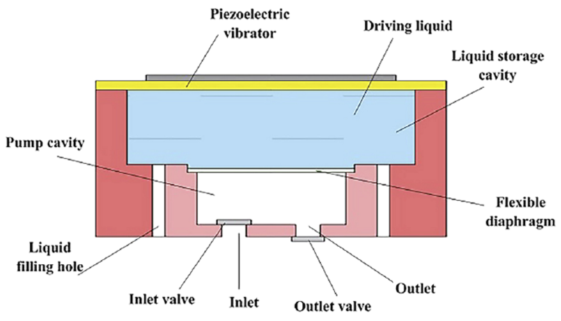
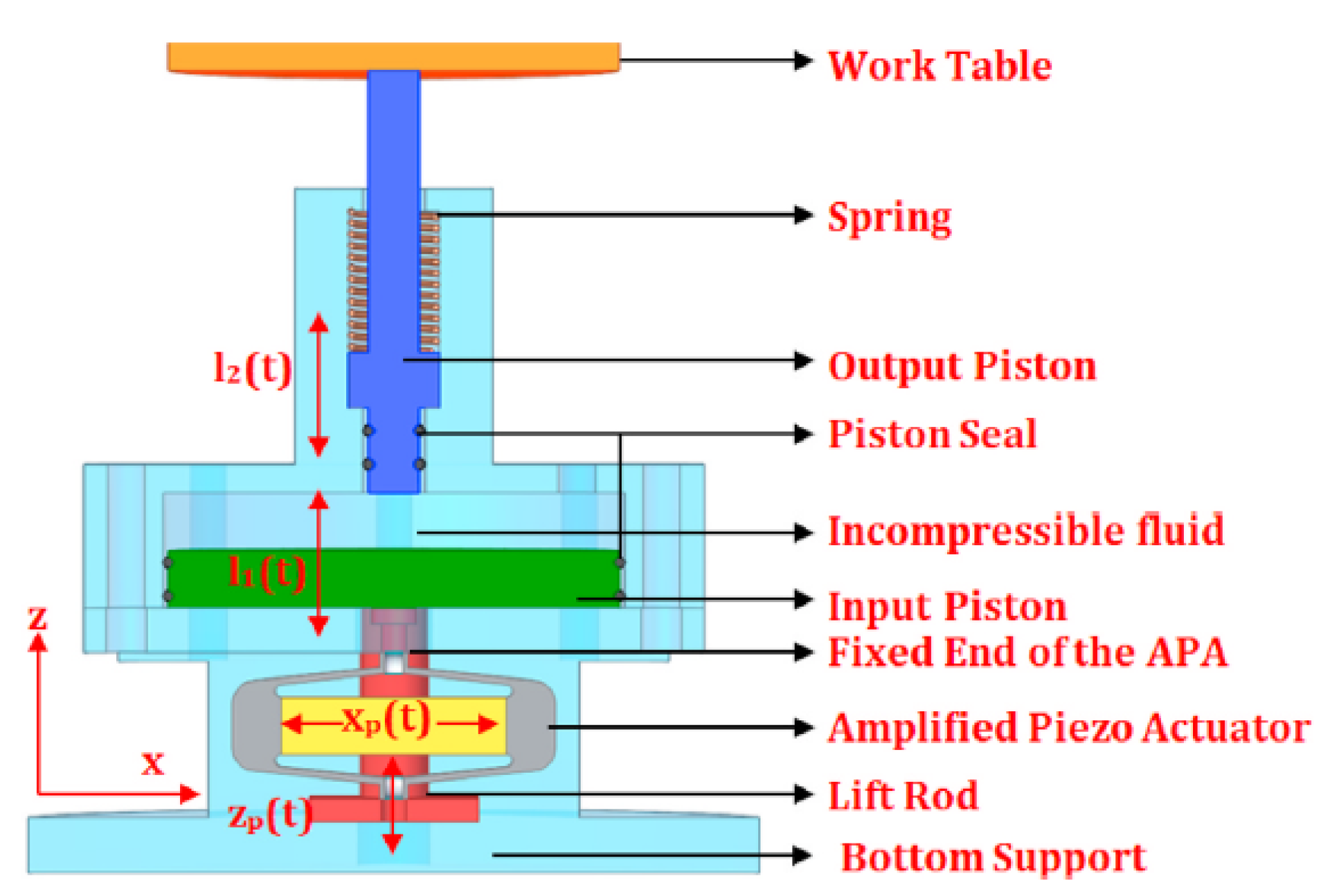
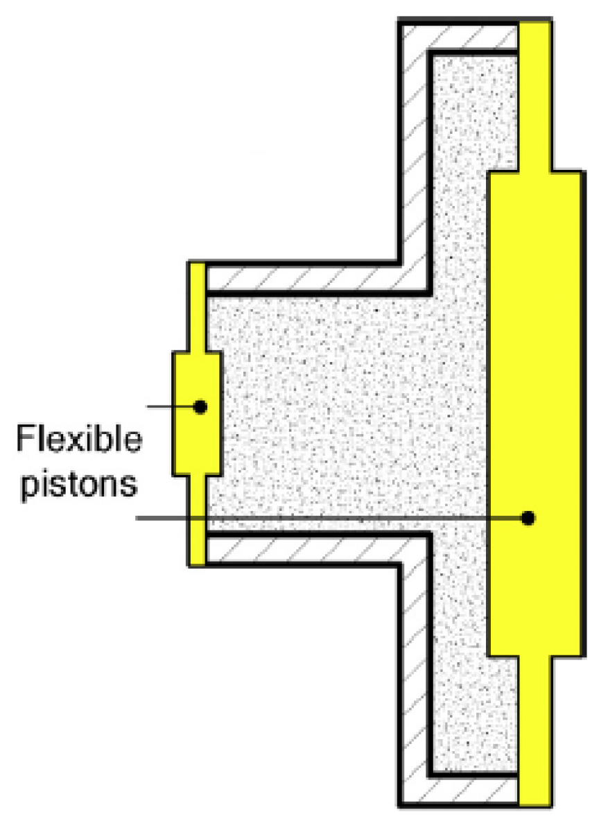
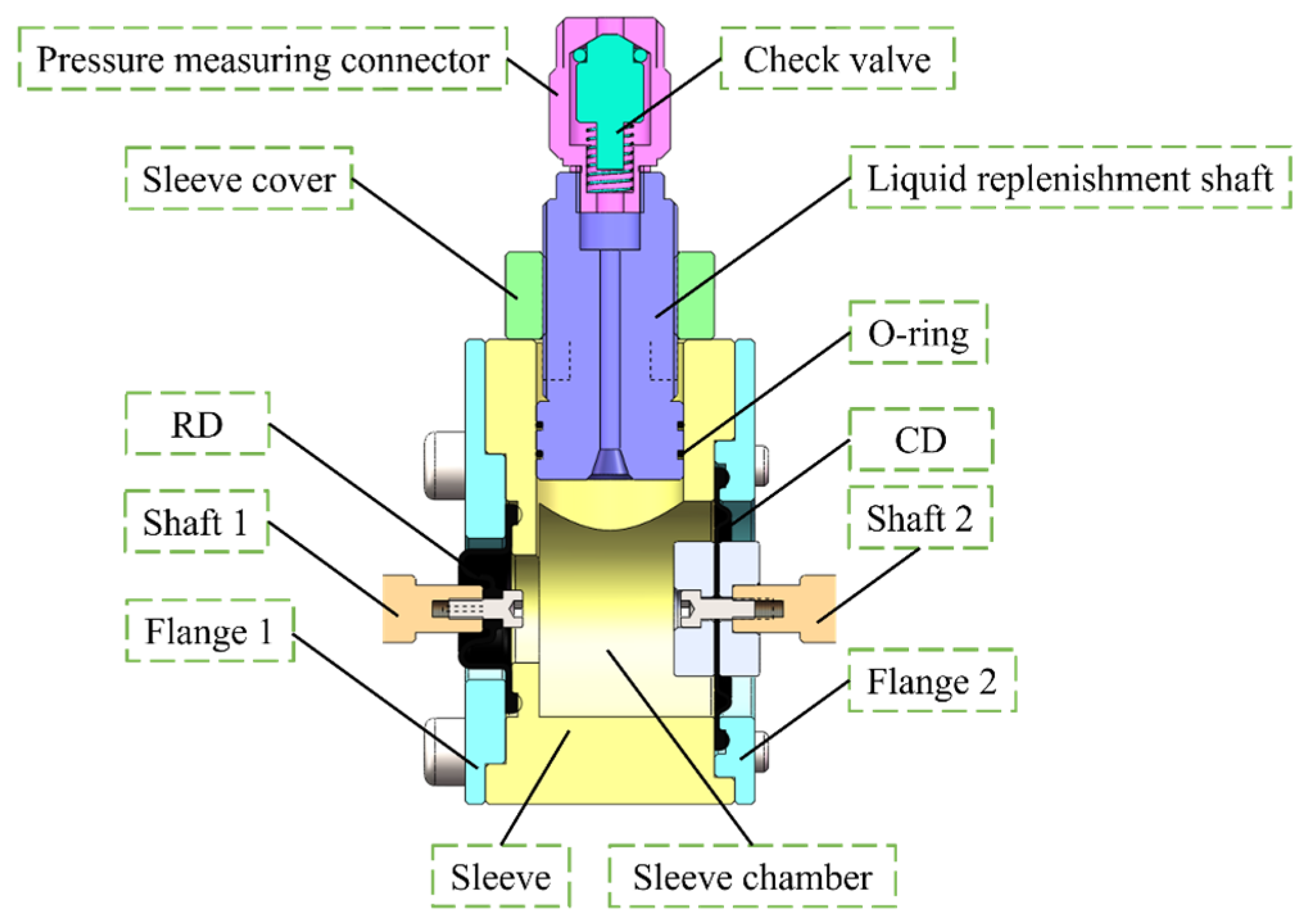
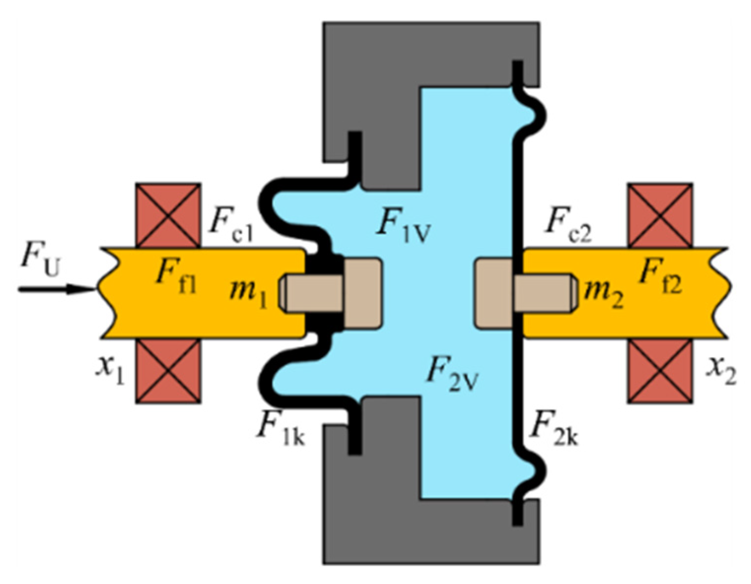
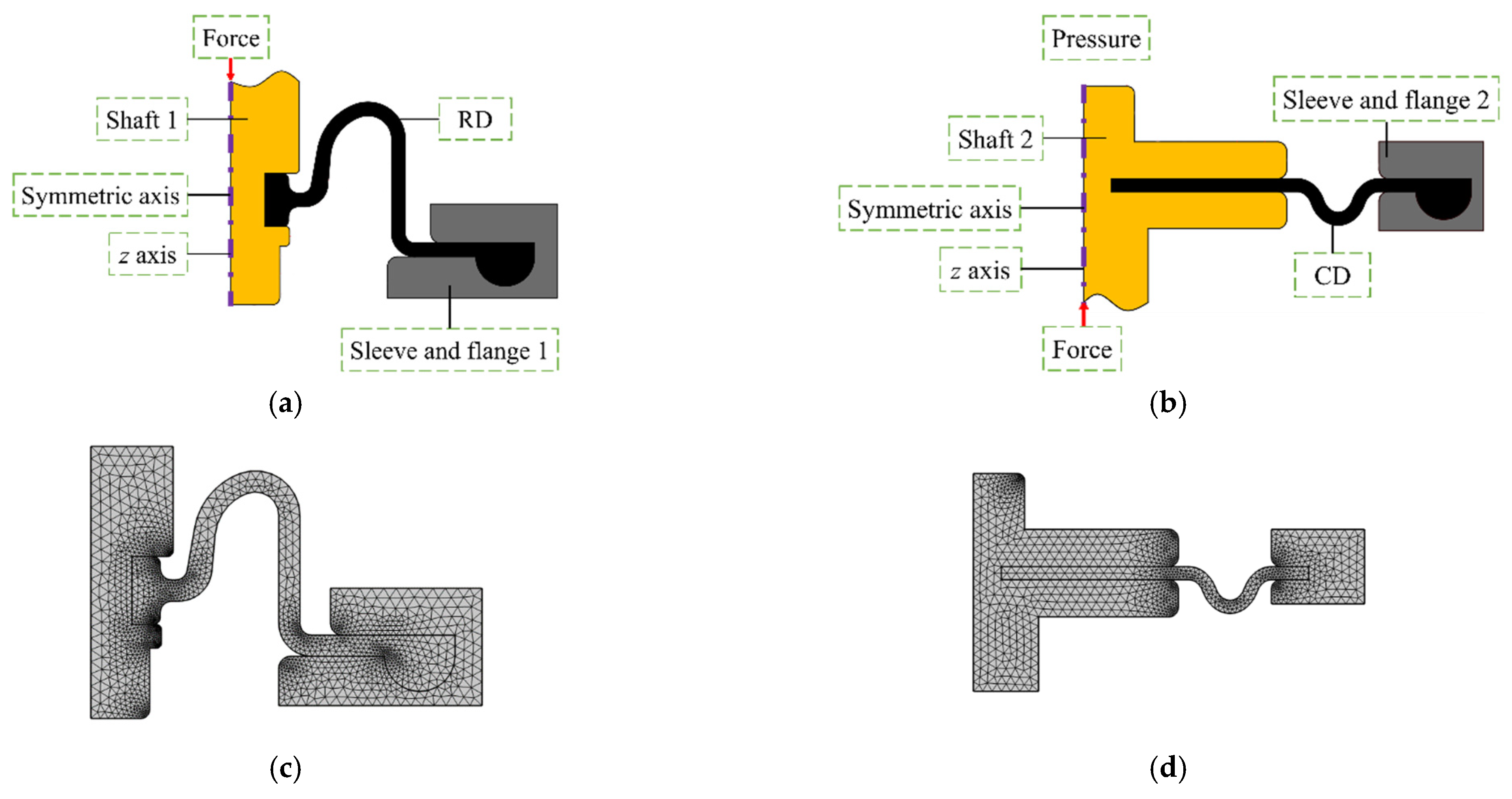
2.1. Working Principle

The working principle of the proposed HFAM is shown in Figure 5. The HFAM is mainly composed of an RD, a CD, a sleeve, a liquid replenishment mechanism, and other connecting mechanisms. The amplification function is achieved using the area difference between the RD and the CD. The RDs [20] and the CDs [21] are diaphragms characterized by a significant linear deformation range and small elastic deformation influence. The RDs exhibit larger volume deformation than the CDs, with the same area. Consequently, the RD is installed at the small diameter end of the HFAM, and the CD is installed at the large diameter end of the HFAM.

The sleeve chamber is filled with liquid, and the sleeve has holes at both ends, featuring a small diameter end of 16 mm and a large diameter end of 32 mm, resulting in a diaphragm area ratio of 1:4. Shaft 1 serves as the input end, connected to the VCM on the left end and linked to the RD on the right end. Shaft 2 serves as the output end, connected to the CD on the left end and attached to the load on the right end. A liquid replenishment device is incorporated to ensure timely replenishment of the liquid in the HFAM without disassembly. The upper end of the sleeve is matched with the head of the liquid replenishment shaft and sealed with O-rings to prevent leakage. The middle section of the liquid replenishment shaft is equipped with an external thread and is connected to the internal thread of the sleeve cover. A through-hole is opened in the middle of the liquid replenishment shaft to connect the sleeve chamber and the pressure measuring connector. The upper end of the pressure measuring connector is connected to the check valve. The mechanisms are used to expel the gas in the HFAM. Specifically, by pressing the check valve while rotating the liquid replenishment shaft clockwise. When there are no bubbles and only liquid flows out from the check valve, it indicates that the gas in the HFAM is completely expelled.

2.2. Mathematical Model

The force state of the HFAM is shown in Figure 6. It is assumed that both rubber and liquid are incompressible. The reduction in the RD volume chamber is equal to the increase in the CD volume chamber. When the VCM propels shaft 1 to the right, the liquid pressure in the sleeve chamber increases. The heightened pressure propels the CD and shaft 2 in the same direction. Throughout the motion, there are static friction forces and viscous friction forces on the shafts, and the diaphragm deformations produce elastic forces.

The axial force balance expressions of the RD and the CD are

$$F_{\mathrm{U}}-F_{1\mathrm{V}}-F_{1\mathrm{k}}-F_{\mathrm{c}1}-F_{\mathrm{f}1}=m_1{\ddot{x}}_1$$

(1)

$$F_{2\mathrm{V}}-F_{2\mathrm{k}}-F_{\mathrm{c}2}-F_{\mathrm{f}2}=m_2{\ddot{x}}_2$$

(2)

where F_U is the driving force of the VCM, F_1V and F_2V are, respectively, the forces applied to the RD and the CD by the liquid, F_1k and F_2k are, respectively, the elastic forces arising from the deformation of the RD and the CD, F_c1 and F_c2 are, respectively, the viscous friction forces of shafts 1 and 2, F_f1 and F_f2 are, respectively, the static friction forces of shafts 1 and 2, x₁ and x₂ are, respectively, the displacements of the RD and the CD, and m₁ and m₂ are, respectively, the masses of the shafts, sensors, and other objects connected to the RD and the CD. Considering that the mass of the fluid in the sleeve chamber is small and the precise motion state is difficult to calculate, the influence of the fluid mass is ignored in the system model.

The output force of the VCM is related to the electric current acting on the VCM, and the expression is

$$F_{\mathrm{U}}=BI{L}_{\mathrm{U}}$$

(3)

where B is the magnetic induction, I is the electric current acting on the VCM, L_U is the length of the coil actuator, and BL_U is the force constant of the VCM, expressed by K_f.

The electric current of the VCM depends on the voltage, and the expression is

$$U=IR+L{\displaystyle \frac{dI}{dt}}$$

(4)

where U is the voltage acting on the VCM, R is the resistance of the VCM, and L is the inductance of the VCM.

The force exerted by the liquid on the RD and the CD depends on their effective areas in the axial direction, and the expression is

$${\displaystyle \frac{F_{1\mathrm{V}}}{F_{2\mathrm{V}}}}={\displaystyle \frac{A_1}{A_2}}=k_{\mathrm{p}2}$$

(5)

where A₁ and A₂ are, respectively, the effective area in the axial direction of the RD and the CD, and k_p2 is the area proportional coefficient.

The elastic forces of the RD and the CD are related to the displacements, and their expressions are

$$F_{1\mathrm{k}}=k_1{x}_1$$

(6)

$$F_{2\mathrm{k}}=k_2{x}_2$$

(7)

where k₁ and k₂ are the elastic slopes of the RD and the CD. They must be determined through finite element simulation.

The viscous friction forces associated with the RD and the CD depend on the speed, and the expressions are

$$F_{\mathrm{c}1}=c_{\mathrm{v}1}{\dot{x}}_1$$

(8)

$$F_{\mathrm{c}2}=c_{\mathrm{v}2}{\dot{x}}_2$$

(9)

where c_v1 and c_v2 are, respectively, the viscous friction coefficients of shafts 1 and 2.

To make the static friction forces of the objects at rest equal to the external forces, the expressions of F_f1 and F_f2 are set to

$$F_{\mathrm{f}1}=\left\{\begin{array}{cc}-\left|{F_{\mathrm{f}1}}^{\prime }\right|& {\dot{x}}_1\le -{\displaystyle \frac{\left|{F_{\mathrm{f}1}}^{\prime }\right|}{k_{\mathrm{s}}}}\\ k_{\mathrm{s}}{\dot{x}}_1& -{\displaystyle \frac{\left|{F_{\mathrm{f}1}}^{\prime }\right|}{k_{\mathrm{s}}}}<{\dot{x}}_1<{\displaystyle \frac{\left|{F_{\mathrm{f}1}}^{\prime }\right|}{k_{\mathrm{s}}}}\\ \left|{F_{\mathrm{f}1}}^{\prime }\right|& {\dot{x}}_1\ge {\displaystyle \frac{\left|{F_{\mathrm{f}1}}^{\prime }\right|}{k_{\mathrm{s}}}}\end{array}\right.$$

(10)

$$F_{\mathrm{f}2}=\left\{\begin{array}{cc}-\left|{F_{\mathrm{f}2}}^{\prime }\right|& {\dot{x}}_2\le -{\displaystyle \frac{\left|{F_{\mathrm{f}2}}^{\prime }\right|}{k_{\mathrm{s}}}}\\ k_{\mathrm{s}}{\dot{x}}_2& -{\displaystyle \frac{\left|{F_{\mathrm{f}2}}^{\prime }\right|}{k_{\mathrm{s}}}}<{\dot{x}}_2<{\displaystyle \frac{\left|{F_{\mathrm{f}2}}^{\prime }\right|}{k_{\mathrm{s}}}}\\ \left|{F_{\mathrm{f}2}}^{\prime }\right|& {\dot{x}}_2\ge {\displaystyle \frac{\left|{F_{\mathrm{f}2}}^{\prime }\right|}{k_{\mathrm{s}}}}\end{array}\right.$$

(11)

where F_f1′ and F_f2′ are the maximum static friction forces of shafts 1 and 2, and k_s is a constant with a value much greater than c_v1 and c_v2. Through this design, the static friction forces can be dynamically and smoothly changed whenever the objects are stable and moving.

Since the reduction in the RD volume chamber is equal to the increase in the CD volume chamber, the expression is

$$V_1=V_2$$

(12)

where V₁ is the reduction in the RD volume chamber, and V₂ is the increase in the CD volume chamber.

The variations in the volume chamber of the RD and the CD are related to their displacements, respectively, and the expressions are

$$V_1=f\left(x_1\right)$$

(13)

$$V_2=f\left(x_2\right)$$

(14)

where f(x₁), f(x₂) are functions related to the displacement that need to be determined through simulation.

The relationship between the displacement of the RD and the displacement of the CD must be defined. Combining with Equations (12)–(14), the displacement proportional coefficient kp1 is defined, and the expression is

$$k_{\mathrm{p}1}={\displaystyle \frac{x_1}{x_2}}$$

(15)

Combining Equations (1)–(15), a dynamic model of the HFAM has been formulated in Simulink, as shown in Figure 7. In the dynamic model, the input is the voltage acting on the voice coil motor, which is converted into the driving force F_U by Equations (3) and (4), and the output is the displacement of the CD x₂. The model can be divided into the RD part and the CD part. The two parts are established based on Equation (1) and Equation (2), respectively, and are connected through Equations (5) and (15).

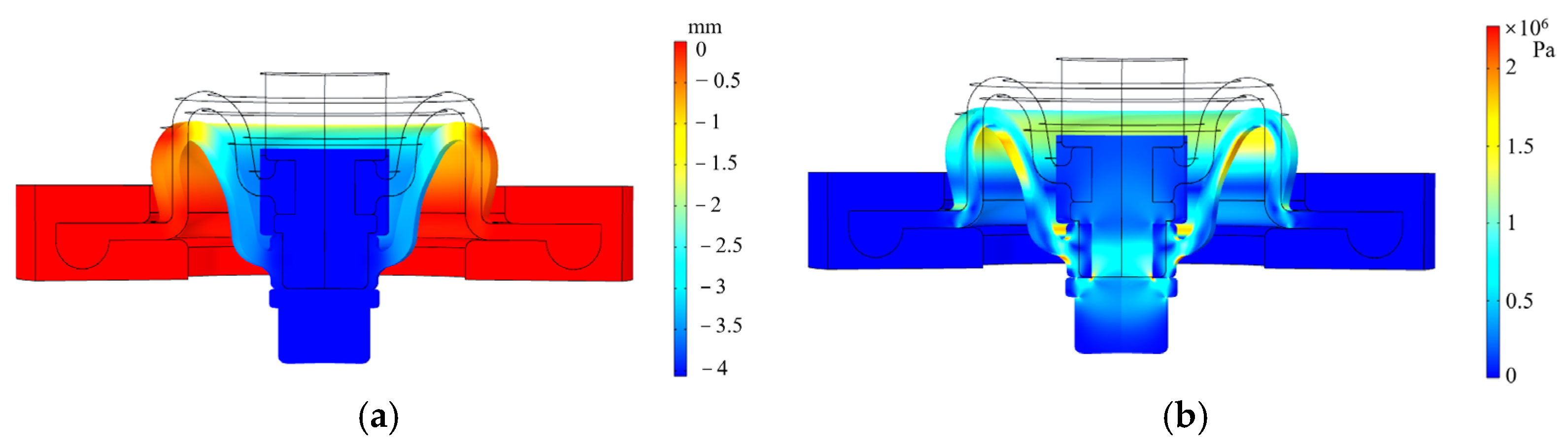
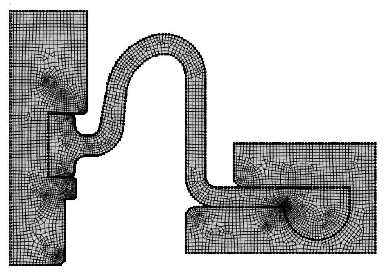
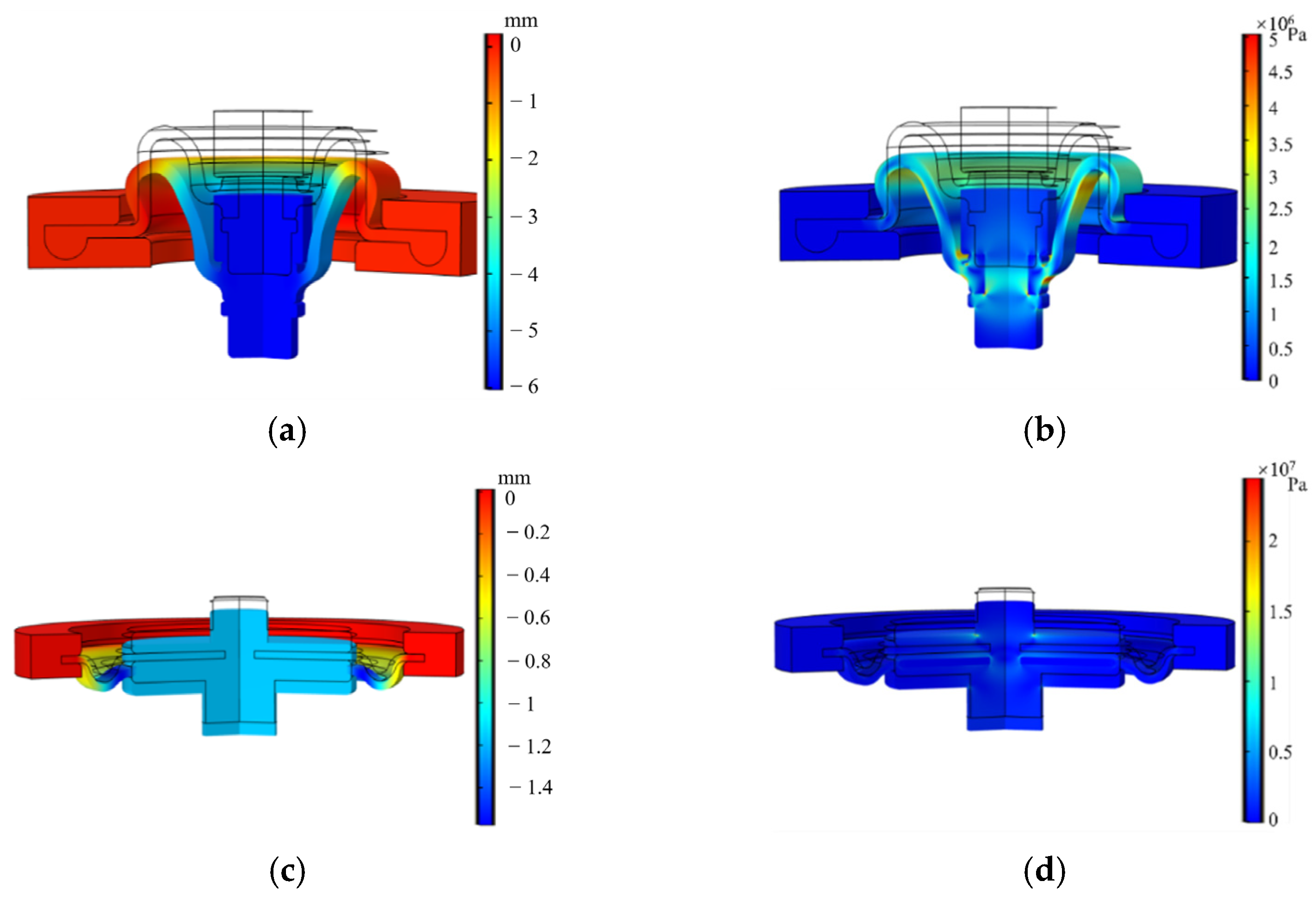
2.3. Diaphragm Mechanical Model

A nonlinear coupling exists between the elastic force of the rubber and the pressure of the liquid when the diaphragm undergoes deformation along its axis. To scrutinize the interplay of the mechanical characteristics between the RD and the CD, finite element simulations were conducted. Due to the assumption that the liquid was incompressible, the pressure could not be transmitted within the sleeve chamber. The RD and the CD were subjected to finite element simulations, respectively. In accordance with the hypothesis, under identical conditions, the reduction in the RD volume chamber was equal to the increase in the CD volume chamber. At the same time, the liquid exerted the same pressure on the diaphragms. In the subsequent analyses, the two simulations could be combined through the same volume and pressure.

Because the diaphragm is cylindrical, a two-dimensional axisymmetric space dimension was employed in the finite element simulation for the diaphragm analysis. The elastic modulus of the rubber is nonlinearly influenced by factors such as material characteristics and dimensions. The Mooney–Rivlin constitutive model is recognized for accurately depicting the hyperplastic characteristics of incompressible rubber materials under small and medium strains [22]. The strain energy density function is

$$W=C_{10}\left(I_1-3\right)+C_{01}\left(I_2-3\right)$$

(16)

where W is the strain energy, I₁ and I₂ are deformation tensors, and C₁₀ and C₀₁ are Mooney constants.

The model effectively characterizes the mechanical characteristics of the rubber materials within a deformation range of less than 150%, thereby satisfying the computational demands applicable to the rubber materials in practice. The relationship between the elastic modulus E and the shear modulus G of rubber materials under the small strain condition is

$$G={\displaystyle \frac{E}{2\left(1+\mu \right)}}$$

(17)

Assuming that rubber is incompressible, Poisson’s ratio μ is 0.5, and Equation (17) can be simplified as

$$G\approx {\displaystyle \frac{E}{3}}=2\left(C_{10}+C_{01}\right)$$

(18)

The ratio of C₀₁ to C₁₀ is a constant, and the expression is

$$k_r={\displaystyle \frac{C_{01}}{C_{10}}}$$

(19)

where k_r is the mechanical characteristic coefficient of the constitutive model. The semi-empirical equation relating Shore hardness and Young’s modulus is [23]

$$E={\displaystyle \frac{2.15s+15.75}{100-s}}$$

(20)

where s is the Shore hardness. In the research, the used diaphragm material is Hydrogenated Nitrile Butadiene Rubber (HNBR) with a Shore hardness of 70 HA.

According to the research of Zhang H [24] et al., the parameter k_r equals 0.25. Combined with Equations (18)–(20), the parameters C₁₀ and C₀₁ are calculated as 0.7388 MPa and 0.1847 MPa, respectively. The rubber material parameters are shown in

Table 1. Rubber material parameters.

Definition	Parameter	Value	Unit
Shore hardness	s	70	HA
Density	ρ	1.3	g/cm3
Mechanical characteristic coefficient of the constitutive model	kr	0.25	-
Model parameter	C10	0.7388	MPa
Model parameter	C01	0.1847	MPa
Elastic modulus	E	5.545	MPa
Poisson’s ratio	μ	0.5	-

, while the other connectors’ material is 304 stainless steel.

Subsequently, finite element simulations were employed for the solid modeling and meshing of the HFAM. As shown in Figure 8, the established simulation models are composed of shafts, diaphragms, sleeve, and flanges. Considering that all these components have axis symmetry about the shafts’ central axes, a two-dimensional axis symmetry model was used for the simulation model. The left ends of shaft 1 and shaft 2 in Figure 8 indicate the central axes of the actual shafts and set the symmetry axes. The boundary conditions of the simulation models are shown in Figure 8a,b. In the simulations of the RD part, there was an acting force added to the upper end of shaft 1, and the force was regarded as being generated by the VCM. The sleeve and flange 1 were set as fixed constraints, and the contact surfaces of the different components were set as contact pairs. In the simulations of the CD part, there was an acting force added to the lower end of shaft 2, and the force was regarded as being generated by the external load. Similar to the RD simulations, the sleeve and flange 2 were set as fixed constraints, and the contact surfaces of the different components were set as contact pairs. In the simulations, the magnitudes of the acting forces were changed, and the displacements of the shafts were recorded.

Considering the complex shapes of the models, the grids of the models were divided by the free triangle mesh function of the COMSOL Multiphysics 6.2 software, as shown in Figure 8c,d. To ensure the accuracy of the results, grid independence tests were carried out. The specific test process was as follows: First, the mesh size parameter was set to four different levels in COMSOL, and the corresponding grids of the RD and CD part models were divided. Second, the test condition was randomly selected, in which the acting forces of the RD and CD parts were 8.7 N and 1.35 N, respectively. Finally, the deformation states of the RD and CD parts under the specified loads were simulated by using the four grids of different sizes mentioned above. Taking the RD part of the No. 3 level grid as an example, the simulation results are shown in Figure 9. The displacements of shafts were measured and used as the criteria to judge the grid independence, and the results are shown in

Table 2. Grid independence tests of finite element simulations.

Grid Independence Test of the RD
Number	Domain Unit	Edge Unit	Displacement	Deviation Rate Compared to the Next Grid
1	4050	432	3.9572 mm	2.48%
2	6136	527	4.0552 mm	2.14%
3	12,437	796	4.1419 mm	1.09%
4	40,262	1414	4.1869 mm	-
Grid Independence Test of the CD
Number	Domain Unit	Edge Unit	Displacement	Deviation Rate Compared to the Next Grid
5	2633	347	1.1599 mm	2.73%
6	3954	421	1.1916 mm	2.24%
7	11,737	695	1.2183 mm	0.84%
8	41,785	1287	1.2285 mm	-

. Generally, in grid independence tests, when the grid deviation rate is below 2%, it is considered the simulation result error is within the acceptable range [24]. Considering the efficiency and the accuracy of the simulation calculation, No. 3 and No. 7 were selected as the research grids.

To judge the influence of the mesh type on simulation accuracy, a quadrilateral grid of the RD part was divided using the same mesh size parameter as No. 3, as shown in Figure 10. The number of quadrilateral grids was 5857 domain units and 816 edge units. The simulation of the RD part model was conducted under the same 8.7 N load force, and the results are shown in Figure 11. The displacement of RD part shaft is 4.072 mm, and the deviation from the free triangle grid is only 0.07 mm. It can be seen that the mesh type has no obvious influence in the research, and the free triangle grids are used uniformly in the following research.

The axial displacement of the RD ranges from −1 mm to 6 mm, while the axial displacement of the CD ranges from −0.12 mm to 1.2 mm. A finite element parametric scanning tool was used to analyze the state of the diaphragm under different forces and pressures. The tensile strength of the HNBR with 70 HA hardness is 18.2 MPa. The safety factor was set to 3 times. The displacement and stress cloud diagrams of the diaphragms are shown in Figure 12. When the displacement of the RD is 6 mm, the maximum stress is 4.78 MPa. When the displacement of the CD is 1.2 mm, the maximum stress is 5.42 MPa. It is less than the tensile strength.

To investigate the elastic characteristics and volume deformation of the diaphragm under the force conditions, finite element simulations were conducted on the diaphragms. Under the two-dimensional axial symmetry, the expression of the diaphragm volume deformation V is

$$V={\displaystyle \int z}\mathrm{d}\sigma$$

(21)

where z is the displacement in the z-direction, and σ is the area of the projection in the z-direction.

The relationships between the displacement, volume, and force of the diaphragms obtained through the simulations and the least squares polynomial fittings are shown in Figure 13.

When the displacement range of the RD is from −1 mm to 4 mm, and the displacement range of the CD is from −0.12 mm to 1.2 mm, the volume deformation of the diaphragms increases with the increase in the diaphragm displacements, and the root mean square errors are 0.011 and 0.0064, respectively. Therefore, Equations (13) and (14) can be expressed as linear equations, and their expressions are

$$V_1=k_{v1}{x}_1$$

(22)

$$V_2=k_{v2}{x}_2$$

(23)

where k_v1 and k_v2 are the elastic slopes of the RD and the CD, respectively.

In the displacement range, k_v1 and k_v2 are obtained by least squares polynomial fittings with values of 0.1336 and 0.5722, respectively. Therefore, combining with Equations (12), (15), (22), and (23), k_p1 is 4.2829. In the same displacement range, the elastic forces of the diaphragms increase with the increase in the diaphragm displacements, and the root mean square errors are 0.6809 and 0.228, respectively. The expressions of the least squares polynomial fittings are

$$F_{1\mathrm{k}}=k_1{x}_1+b_1$$

(24)

$$F_{2\mathrm{k}}=k_2{x}_2+b_2$$

(25)

where k₁, b₁, k₂, and b₂ are 2.182, 0.052, 1.13, and 0.018, respectively.

Because the fitted intercepts are close to 0 compared to the magnitudes of the diaphragm elastic forces, they can be ignored.

3. Experimental Research and Discussion

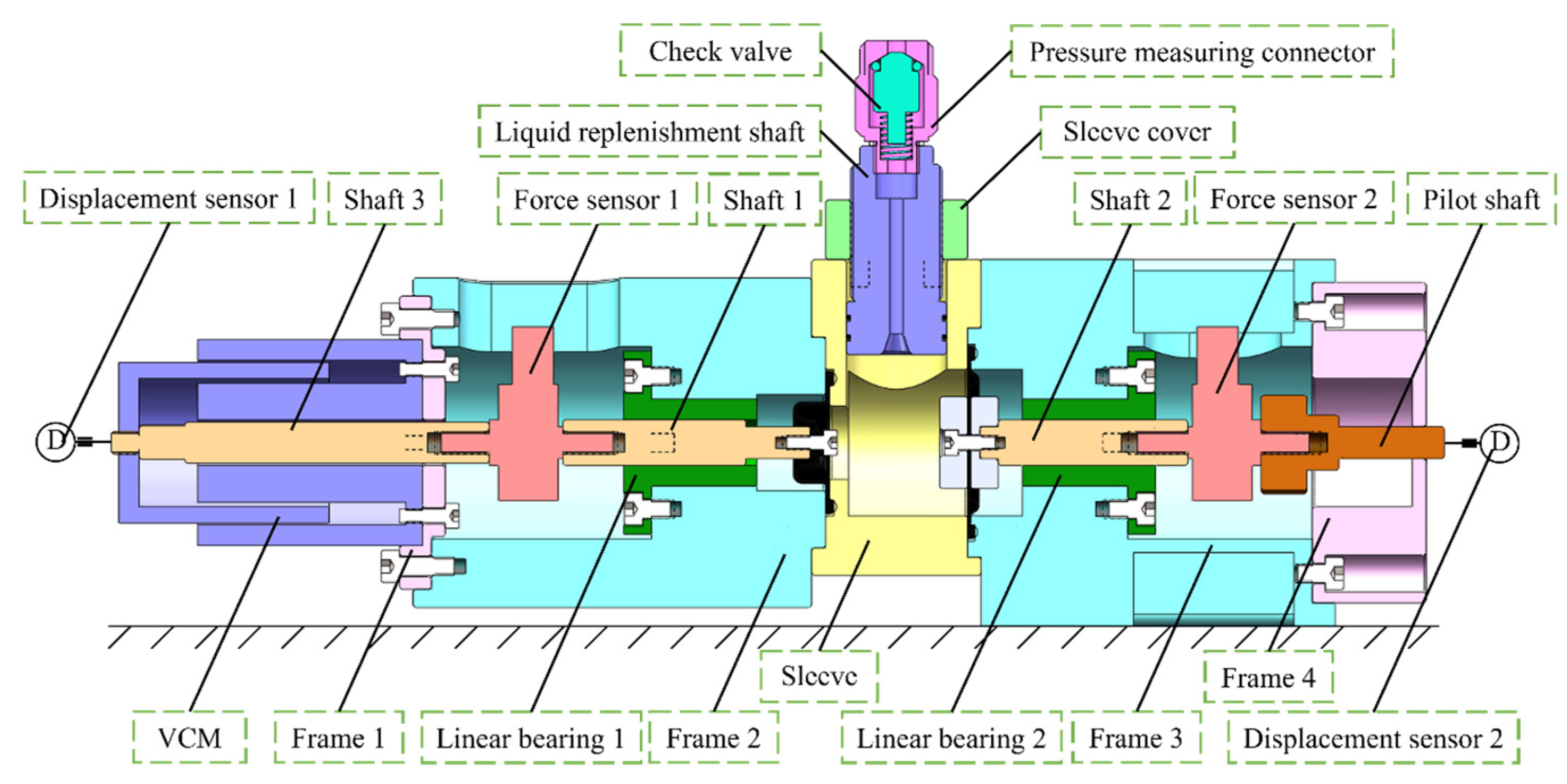
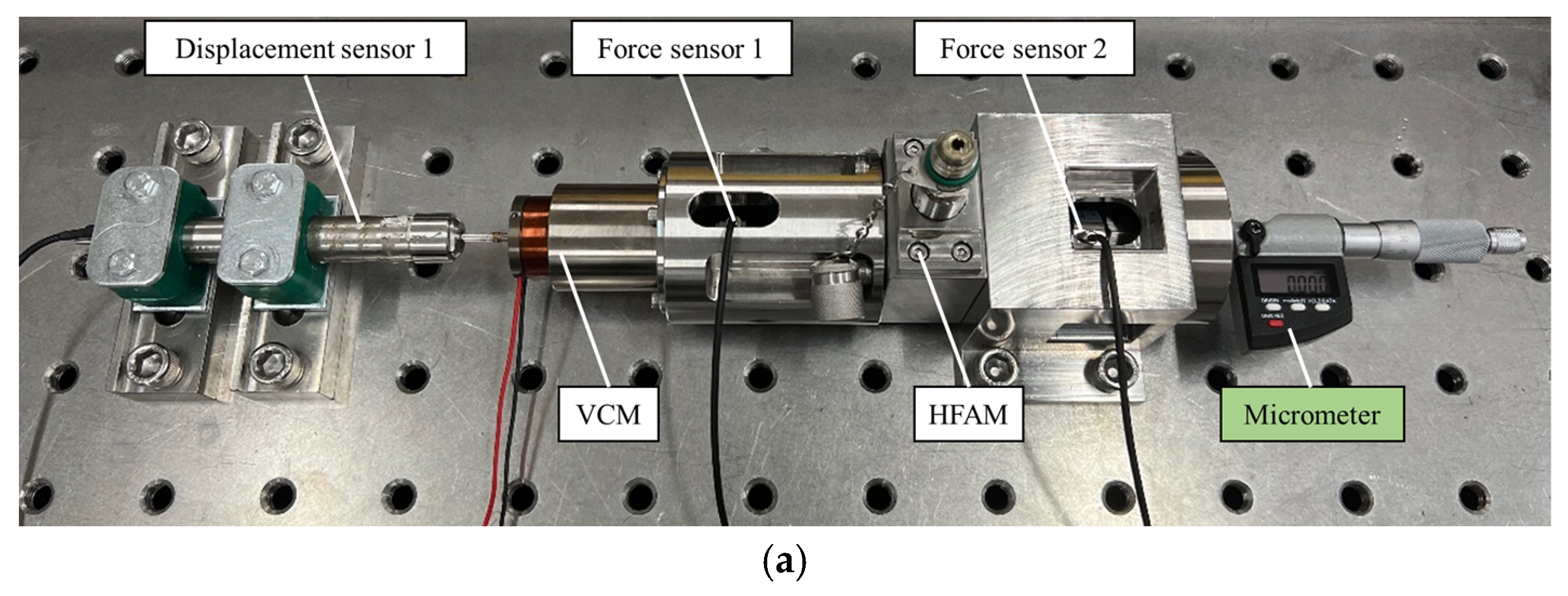
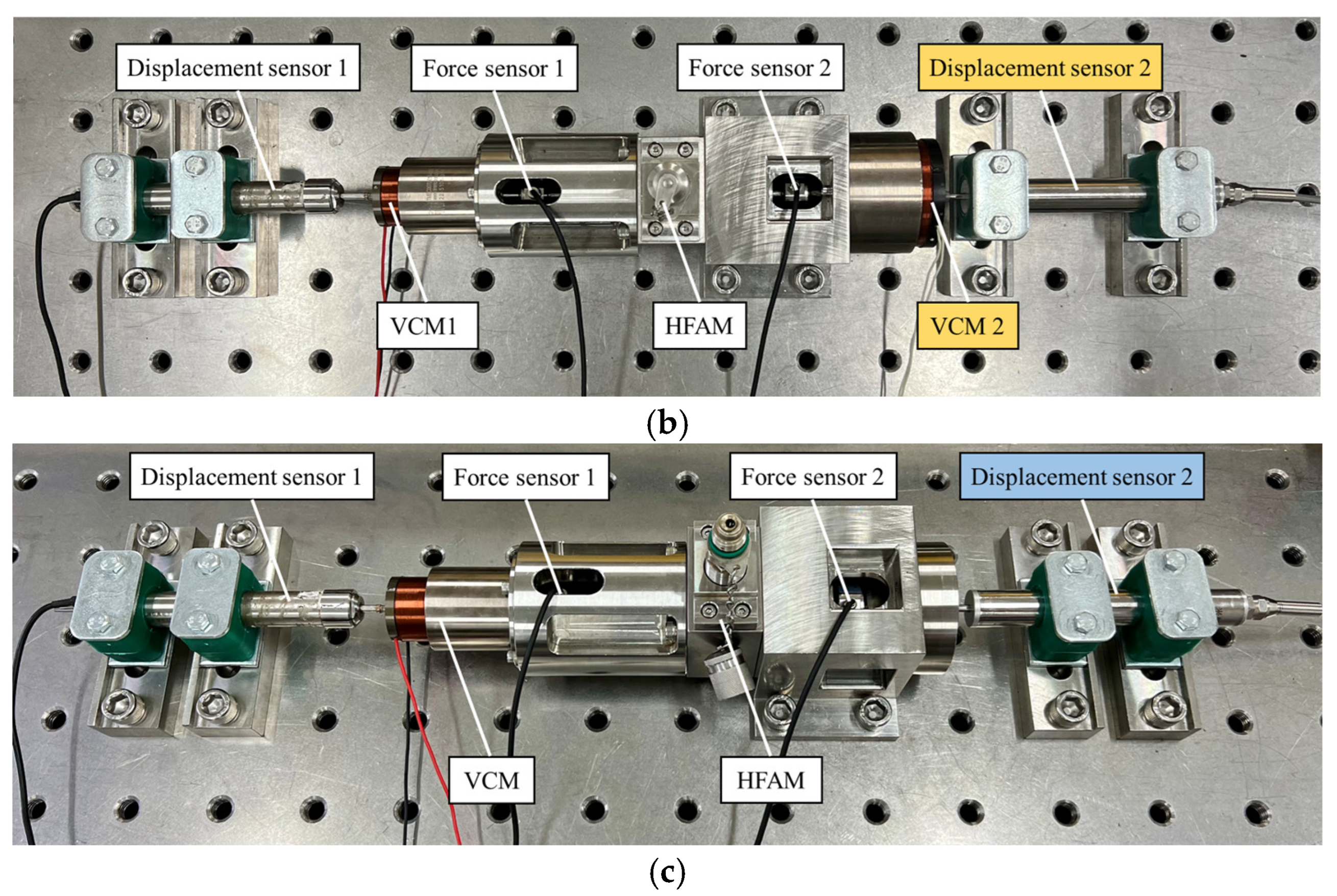
3.1. Experimental System

To analyze the relationships between the force and the displacement of the HFAM, the experimental system of the HFAM was set up as shown in Figure 14. The coil actuator of the VCM was connected to force sensor 1 through shaft 3, force sensor 1 was connected to the RD through shaft 1, force sensor 2 was connected to the CD through shaft 2, and the pilot shaft was connected to the right end of force sensor 2. Displacement sensors 1 and 2 measured the displacements of the VCM and the pilot shaft, respectively. Force sensors 1 and 2 measured the forces of the RD and the CD, respectively. The coaxial of the experimental device was ensured through the linear bearings and the positioning circles of the frames. Before the experiment, the sleeve chamber of the HFAM was filled with liquid, the check valve in the pressure measuring connector was compressed, and the liquid replenishment shaft was rotated. When no bubbles emerged from the pressure measuring connector, and only liquid flowed out, it was considered that the sleeve chamber was filled with liquid. The VCM parameters are shown in

Table 3. Parameters of the VCM.

Definition	Parameter	Value	Unit
Force constant	Kf	24.55	N/A
Resistance	R	6.8	Ω
Inductance	L	2.5 × 10−3	H
Displacement range	s1	15	mm
Peak force	Fp	70	N
Continuous force	Fcon	27.5	N

, and the sensor parameters are shown in

Table 4. Parameters of the sensors.

Sensor Type	Voltage Range	Measuring Range	Accuracy
Displacement sensor 1	0–5 V	0–15 mm	1‰
Displacement sensor 2	0–10 V	0–10 mm	1‰
Force sensor 1	−10–10 V	−50–50 N	1‰
Force sensor 2	−10–10 V	−100–100 N	1‰

.

3.2. Results and Discussion

The static and dynamic characteristics of the HFAM were analyzed through simulations and experiments. The experimental system of the HFAM in Figure 14 was subjected to a static experiment, friction force measurement, and dynamic experiment, as shown in Figure 15.

3.3. Static Characteristic

In the static characteristics experiment, the influence of different diaphragm displacements on the trend of the FAR, and the diaphragm displacement ranges with different FARs, were analyzed. In addition, the influence of the initial volume on the relationships between the force and displacement of the HFAM was discussed. The static characteristics experiment system was set up as shown in Figure 15a. Displacement sensor 2 was substituted with a micrometer. The micrometer was located at the right end of the experimental system and connected to frame 4 by a thread. The micrometer was in contact with the pilot shaft of force sensor 2 and limited the displacement of the CD to the right. The set displacement of the CD was changed by adjusting the micrometer. When the pilot shaft was in contact with the micrometer, the pressure in the sleeve chamber increased, the CD was subjected to a larger force, and the FAR was realized.

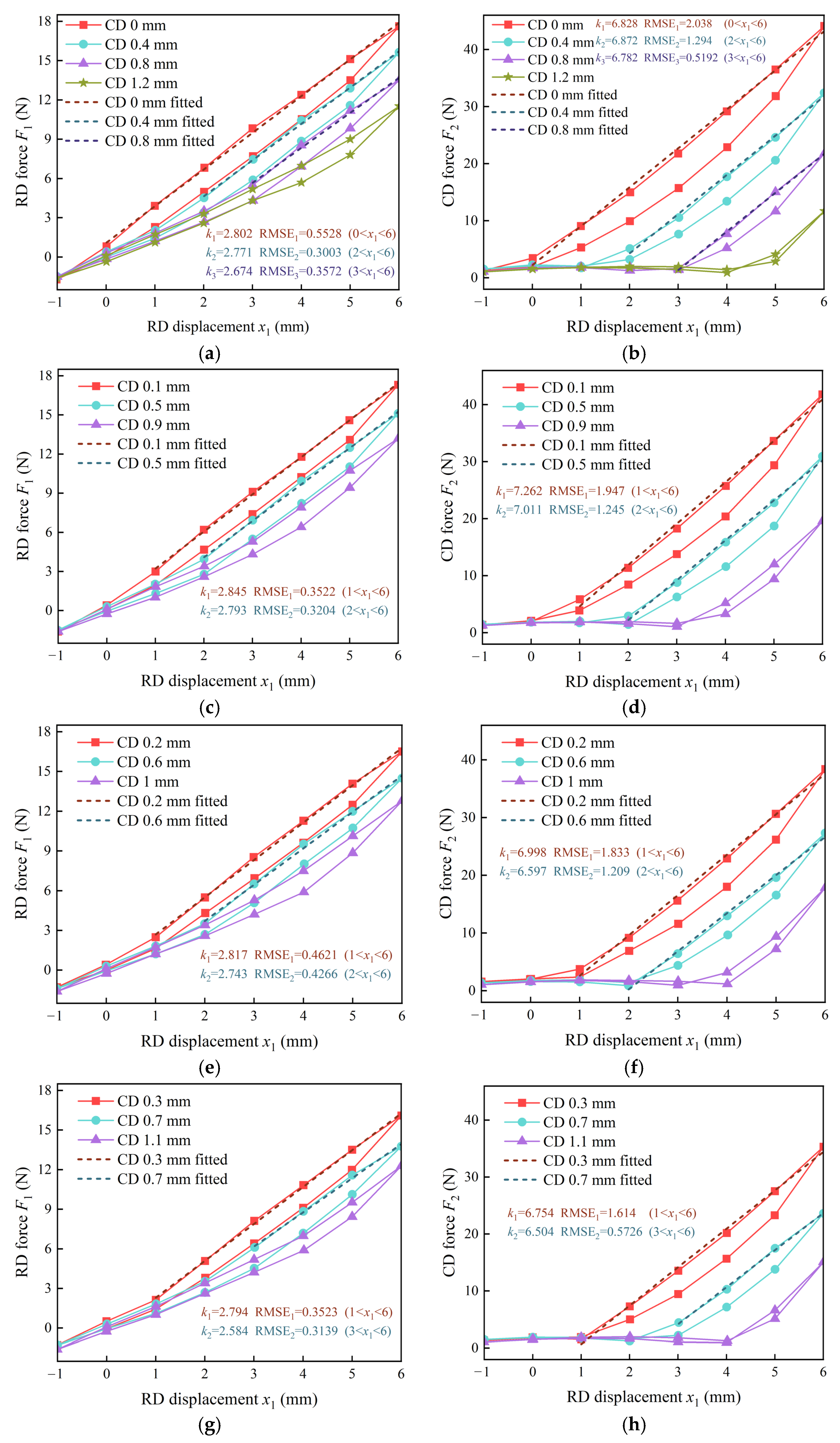
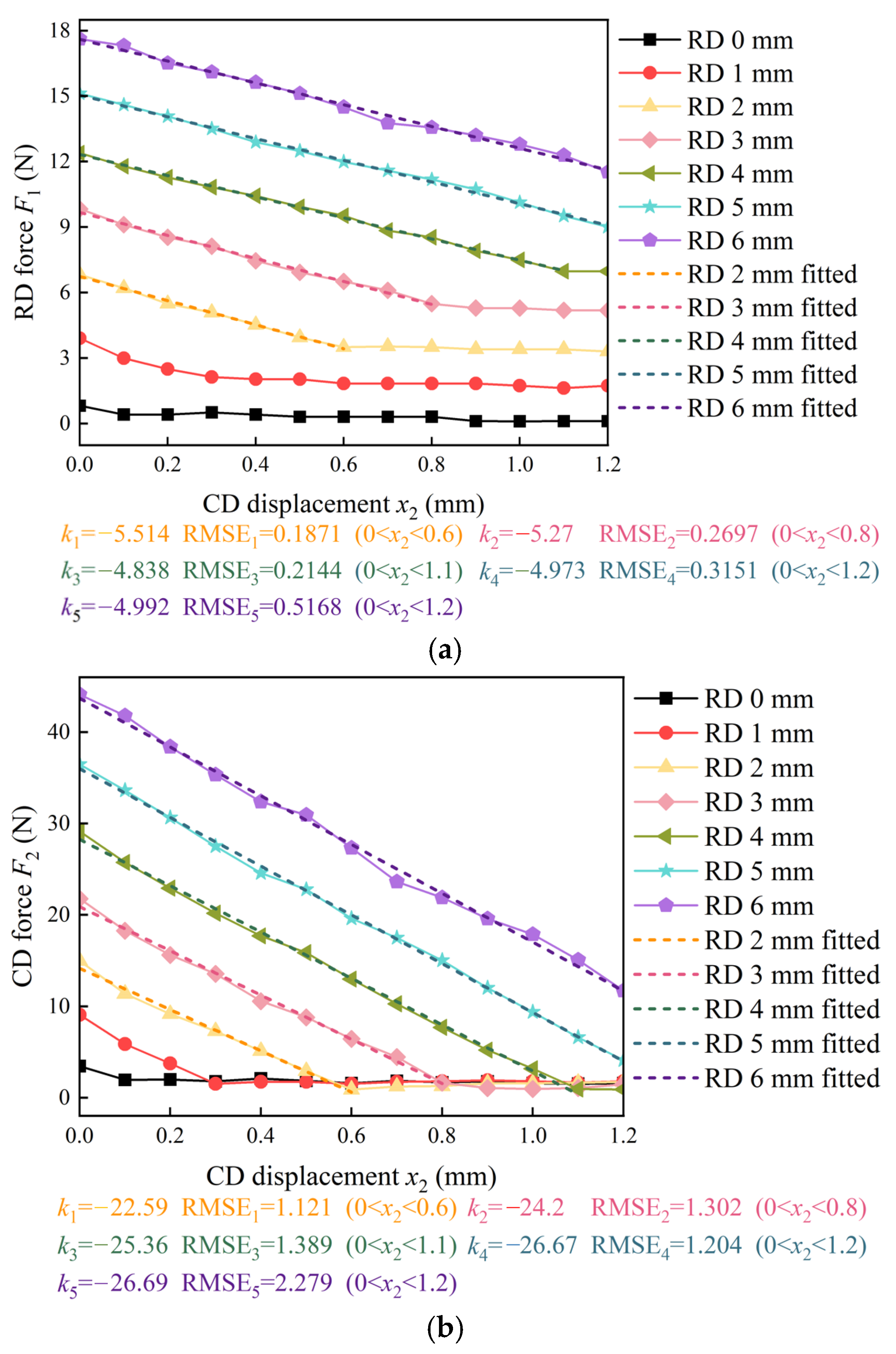
3.3.1. Influence of Different Diaphragm Displacements

The experimental conditions of different diaphragm displacements were that the displacement of the CD started from 0 to 1.2 mm and increased by 0.1 mm for each group. The coil actuator displacement of the VCM was controlled by PID. The VCM moved from −1 mm to 6 mm and back to −1 mm in 1 mm intervals.

In the static experiments of different RD displacements, when the set displacement of the CD was unchanged, there were 13 set displacements of the CD, in a range from 0 to 1.2 mm, as shown in Figure 16. When the displacement of the RD is 6 mm, and the displacement of the CD is 0, the maximum force of the RD is 17.6 N, and the maximum force of the CD is 44.1 N.

When the CD does not reach the set displacement, the force of the CD is basically zero. When the CD reaches the set displacement, the forces of the diaphragms increase with the increase in the RD displacement. When the set displacement range of the is CD from 0 to 0.8 mm, after least squares polynomial fittings, the average slope of the is RD 2.7581 N/mm, the maximum root mean square error is 0.5528, and the maximum slope deviation is 9.17%. The average slope of the CD is 6.8453 N/mm, the maximum root mean square error is 2.038, and the maximum slope deviation is 10.44%. When the set displacement of the CD was from 0.9 mm to 1.2 mm, the experimental points were not discussed, because there were too few experimental points, and there was no reference value.

There is hysteresis in the axial reciprocating motion of the diaphragm, and the hysteresis decreases with the increase in the CD displacement. The hysteresis of the RD is reduced from 2.13 N to 1.5 N, and that of the CD is reduced from 6.28 N to 3.38 N. Hysteresis exists because there are friction forces between the shafts and the linear bearings during the diaphragm movements. Additionally, there is hysteresis in the diaphragm deformation. The larger the deformation of the diaphragm, the larger the hysteresis.

In the static experiments of different CD displacements, when the set displacement of the RD was unchanged, there were 7 set displacements of the RD in a range from 0 to 6 mm, as shown in Figure 17.

When the RD reaches the set displacement, the forces of the diaphragms decrease with the increase in the CD displacement. When the set displacement range of the RD is from 2 to 6 mm, after least squares polynomial fittings, the average slope of the RD is −5.1174 N/mm, the maximum root mean square error is 0.5168, and the maximum slope deviation is 12.26%. When the average slope of the CD is −25.102 N/mm, the maximum root mean square error is 2.279, and the maximum slope deviation is 15.36%. When the set displacement of the RD was 0 and 1 mm, the experimental points were not discussed, because there were too few experimental points, and there was no reference value.

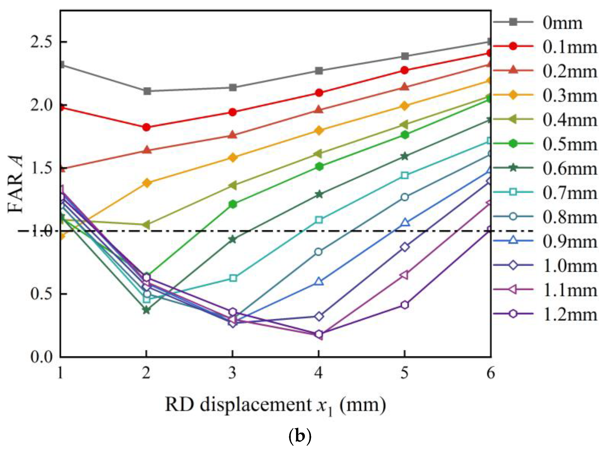
3.3.2. Experimental Analysis of FAR

The FAR is an important performance indicator in the HFAM, which expresses the ratio between the output force and the input force, and the expression of the FAR A is

$$A={\displaystyle \frac{F_2}{F_1}}$$

(26)

where F₁ and F₂ are the input force and the output force of the HFAM, respectively.

During the movement of the VCM, there is a hysteresis loop between the shafts and the linear bearings. By calculating the average value of the HFAM input force and output force during the forward and reverse motion of the VCM, the three-dimensional diagram of the FAR is obtained through Equation (26), as shown in Figure 18a. Figure 18a is projected onto the YZ plane, and the FAR changes with the displacements of the diaphragms, as shown in Figure 18b.

When the displacement of the RD is less than 2 mm, input and output forces are small. They are affected by friction forces, resulting in obvious fluctuations in the FAR. Meanwhile, when the displacements of the RD exceed 2 mm, in most working conditions, the FARs increase with the increase in the RD displacement but decrease with the increase in the CD displacement. When the displacement of the CD is 0 and that of the RD is 6 mm, the maximum FAR of the HFAM is 2.5.

When the set displacement of the CD remained unchanged, the working conditions with the CD set displacements of 0, 0.8, and 1.2 mm were selected, as shown in Figure 18b. When the set displacement of the CD is 0, the displacement of the RD increases from 1 mm to 2 mm, and the FAR decreases from 2.32 to 2.14. When the displacement of the RD increases from 2 mm to 6 mm, the FAR increases from 2.14 to 2.5. When the set displacement of the CD is 0.8 mm, the displacement of the RD increases from 1 mm to 3 mm, and the FAR decreases from 1.2 to 0.3. When the displacement of the RD increases from 3 mm to 6 mm, and the FAR increases from 0.3 to 1.61. When the set displacement of the CD is 1.2 mm, the displacement of the RD increases from 1 mm to 4 mm, and the FAR decreases from 1.27 to 0.18. When the displacement of the RD increases from 4 mm to 6 mm, and the FAR increases from 0.18 to 1.01.

The reason why the FAR first decreases and then increases is that when the displacement of the RD is small, the deformation of the CD is small, so the displacement of the pilot shaft of the CD is not enough to contact the micrometer. At this time, although the pilot shaft is not in contact with the micrometer, the little displacement causes friction on the pilot shaft, which is recorded by the force sensor. Meanwhile, due to the significant deformation of the RD, the force of the RD increases significantly, resulting in a decrease in the FAR. When the pilot shaft is in contact with the micrometer, the force of the CD increases significantly after being amplified by the HFAM. The larger the displacement of the RD, the greater the FAR.

The three planes with FARs of 1, 1.5, and 2 intersect with the curved surface of the FARs to form three intersection lines. These lines represent the critical diaphragm displacement curves of the corresponding FARs, as shown in Figure 19. Through least squares polynomial fittings, three critical curves with FARs of 1, 1.5, and 2 were fitted, and the expression is

$$\left\{\begin{array}{l}A=1:x_2=0.01885x_1^4-0.3043x_1^3+1.788x_1^2-4.314x_1+4.021\\ A=1.5:x_2=0.008885x_1^2+0.07746x_1+0.009964\\ A=2:x_2=0.006457x_1^3-0.03382x_1^2+0.0583x_1-0.03243\end{array}\right.$$

(27)

The displacement ranges of the diaphragms with different FARs are shown in

Table 5. Displacement ranges of diaphragms with different FARs.

Relationships Between RD Displacement x1 and CD Displacement x2	FAR A Ranges
x2 ≥ 0.01885x14 − 0.3043x13 + 1.788x12 − 4.314x1 + 4.021	A < 1
0.008885x12 + 0.07746x1 + 0.009964 ≤ x2 < 0.01885x14 − 0.3043x13 + 1.788x12 − 4.314x1 + 4.021	1 ≤ A < 1.5
0.006457x13 − 0.03382x12 + 0.0583x1 − 0.03243 ≤ x2 < 0.008885x12 + 0.07746x1 + 0.009964	1.5 ≤ A < 2
x2 ≤ 0.006457x13 − 0.03382x12 + 0.0583x1 − 0.03243	2 ≤ A ≤ 2.5

. It can guide users to select a reasonable displacement range of the diaphragm, according to the required FAR.

3.3.3. Influence of Initial Volume

The initial volume of the HFAM sleeve chamber is an essential factor affecting the mechanical characteristics of the system. The initial volume can be changed by rotating the liquid replenishment shaft. The influences of different initial volumes on the mechanical characteristics of the diaphragms are shown in Figure 20. The set displacement of the CD is 0, and the rotation angle of the liquid replenishment shaft ranges from 0 to 360 degrees, with an interval of 180 degrees. The control procedure for the VCM is consistent with the static experiments of different diaphragm displacements in Section 3.3.1.

In the static experiments of different initial volumes, when the displacement of the RD is 6 mm, and the rotation angle is 360 degrees, the maximum force of the RD is 23.4 N, and the maximum force of the CD is 59.5 N.

The forces of the diaphragms increase with the increase in the RD displacement and increase with the increase in the initial volume. After the least square polynomial fittings, the average slope of the RD is 3.045 N/mm, the maximum root mean square error is 0.731, and the maximum slope deviation is 10.81%. The average slope of the CD is 6.939 N/mm, the maximum root mean square error is 1.822, and the maximum slope deviation is 5.17%. When the displacement of the RD is 6 mm, the liquid replenishment shaft is rotated in 180-degree intervals, the average force of the RD increases by 2.7 N, and the average force of the CD increases by 8.1 N.

There is hysteresis in the axial reciprocating motion of the diaphragm. The maximum hysteresis of the RD is 2.23 N, 2.09 N, and 2.12 N, respectively, and the maximum hysteresis deviation is 6.28%. The maximum hysteresis of the CD is 6.49 N, 6.59 N, and 6.72 N, respectively, and the maximum hysteresis deviation is 3.42%.

3.4. Dynamic Characteristic

The static characteristics experiment found that friction force existed when the experimental system was running. Before the dynamic characteristic experiments, it was important to identify the friction parameters. The friction force experiment system was set up as shown in Figure 15b. The pilot shaft was replaced by the VCM2, and the coil actuator displacement of the VCM2 was measured by displacement sensor 2. The RD and the CD were removed, and shafts 1 and 2 remained free. There was no liquid in the sleeve chamber, and it was connected to the atmosphere.

To simulate the static friction forces of the RD and the CD, under a sinusoidal signal with a frequency of 0.1 Hz, the displacement range of the VCM 1 was set from −1 mm to 1 mm, while that of the VCM 2 was set from −0.5 mm to 0.5 mm. In these conditions, the motion speeds of the diaphragms are very slow, and the friction forces acting on the diaphragms are regarded as the static friction forces. Specifically, the static friction forces of the RD and CD are obtained by averaging the data collected by the force sensor during the motions in one direction. The static friction forces of the RD and the CD were measured as 2.5 N and 0.2 N, respectively. Furthermore, the static friction forces were introduced into the Simulink model and simulation tests with sinusoidal voltage input of 1 Hz and 10 Hz were carried out. The displacements of the diaphragms in the simulation were compared with the experiments, and the viscous friction coefficients were manually adjusted to make the motion amplitudes of the simulations and experiments the same. The viscous friction coefficients of the RD and CD were obtained as 55 N·s/m and 27 N·s/m, respectively. A dynamic characteristics simulation was carried out based on the Simulink model in Section 2, and the simulation parameters are shown in

Table 6. Simulink simulation parameters.

Definition	Parameter	Value	Unit
Force constant	Kf	24.55	N/A
Resistance	R	6.8	Ω
Inductance	L	2.5 × 10−3	H
Total mass of the RD end	m1	0.17189	kg
Total mass of the CD end	m2	0.13383	kg
Static friction force of the RD end	Ff1	2.5	N
Static friction force of the CD end	Ff2	0.2	N
RD elastic slope	k1	2.182	N/mm
CD elastic slope	k2	1.13	N/mm
Displacement proportional coefficient	kp1	4.2829	-
Area proportional coefficient	kp2	0.25	-
Viscous friction coefficient of the RD	cv1	55	N·s/m
Viscous friction coefficient of the CD	cv2	27	N·s/m

.

To validate the accuracy of the Simulink simulation, dynamic characteristics experiments were conducted. The dynamic experiment is shown in Figure 15c. The VCM coil actuator executed sinusoidal movement ranging from −1 V to 3 V at frequencies of 0.1 Hz, 0.3 Hz, 0.5 Hz, 0.7 Hz, 1 Hz, 3 Hz, 5 Hz, 7 Hz, and 10 Hz with an inertial load. The displacement of the CD was measured and recorded as the system output. The sampling rate of the experimental points was 10,000 Hz. The frequency sweep method was employed for the Simulink simulation under identical working conditions.

To compare the magnitude ratio and the phase difference between the voltage signals and the displacement signals, they were converted into dimensionless quantities. The magnitude at each frequency was converted to a ratio relative to the Simulink simulation magnitude at 0.1 Hz. Dimensionless dynamic characteristic curves with frequencies of 0.1 Hz, 1 Hz, and 10 Hz were selected, as shown in Figure 21.

According to the dimensionless dynamic characteristic curves shown in Figure 21, the Bode diagram of the dynamic experiments and Simulink simulations in the frequency range from 0.1 Hz to 10 Hz were plotted, as shown in Figure 22.

The experimental magnitude ranges from 0.05 dB to −8.27 dB, and the phase ranges from −21.27 degrees to −62.28 degrees. The Simulink simulation magnitude ranges from 0 to −8.24 dB, and the phase ranges from −21.6 degrees to −80.28 degrees. When the frequency is less than 1 Hz, the maximum magnitude deviation between the simulation value and the experimental value is 0.35 dB, and the maximum phase deviation is 3.04 degrees. When the frequency is greater than 1 Hz, the maximum magnitude deviation between the simulation value and the experimental value is 1.14 dB, and the maximum phase deviation is 21.96 degrees. Therefore, in future dynamic experimental research, the Simulink model for the HFAM can be used to control the load movement. For example, spool movement can be controlled based on the Simulink model of the HFAM.

It is worth noting that the research still has some limitations. At present, the HFAM is mainly suitable for working conditions at normal temperature and pressure and with small input force, such as amplifying the driving force of the electro-mechanical converter in the hydraulic control valve. However, when the HFAM is used in some extreme conditions, such as a very high input force resulting in a large deformation of the diaphragms or a large fluid pressure in the sleeve, the HFAM may have problems, such as diaphragm damage, and thus the failure of the amplification effect. In addition, in this research, it is assumed that the HFAM system is under a fixed temperature of 20 °C and a standard atmospheric pressure environment, and the influence of ambient temperature and air pressure on the working effect of the amplifier is not considered in the model. In actual working conditions, the change in temperature affects the physical property parameters of the diaphragms, for example, the hardness and elastic modulus of the diaphragms decrease with the increase in temperature, and then affect the elastic force generated by the diaphragms. The ambient pressure directly acts on the outer surfaces of the diaphragms, driving the diaphragms to produce elastic deformations and affecting the HFAM’s amplification effect. In subsequent research, factors such as temperature and pressure could be added to the model to further improve the accuracy of the model to adapt to different working conditions.

In addition, this research only deals with a HFAM with specific structure size and does not discuss the influence of RD and CD size parameters on the working effect of HFAMs. In the subsequent research, the influence of the diaphragm size parameters on the working effect of HFAMs could be studied through simulation and experiment methods. Based on the study results, the working effect of HFAMs can be optimized by adjusting the diaphragms’ sizes when facing different working conditions and requirements.

4. Conclusions

This research introduces a HFAM which is composed of an RD and a CD. The HFAM supports a non-coaxial connection between the actuator and the load. A liquid replenishment device is incorporated to ensure timely replenishment of the liquid in the HFAM without disassembly. The dynamic model, based on the force balance method, was established in the Simulink, and the diaphragm forces were obtained by finite element simulations. Moreover, the experimental system was deployed to analyze the static and dynamic characteristics of the HFAM prototype. From this research, the conclusions could be obtained as follows:

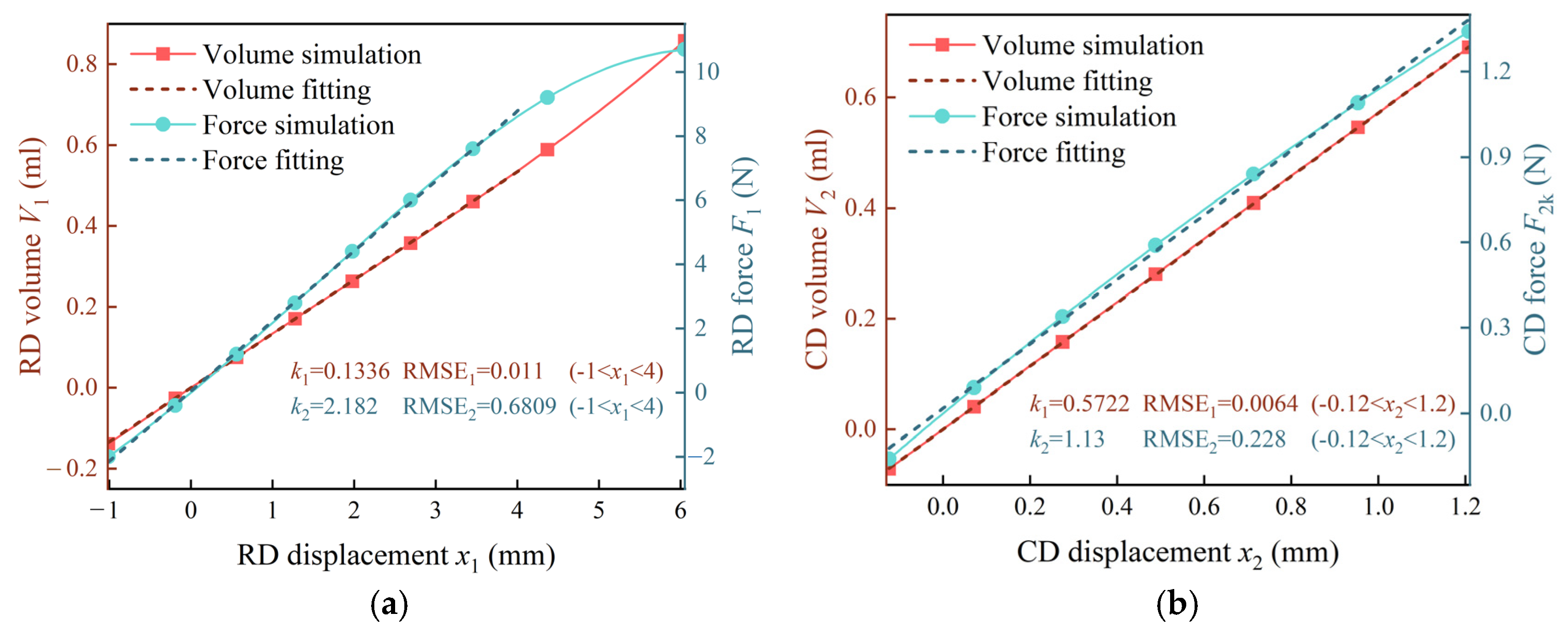
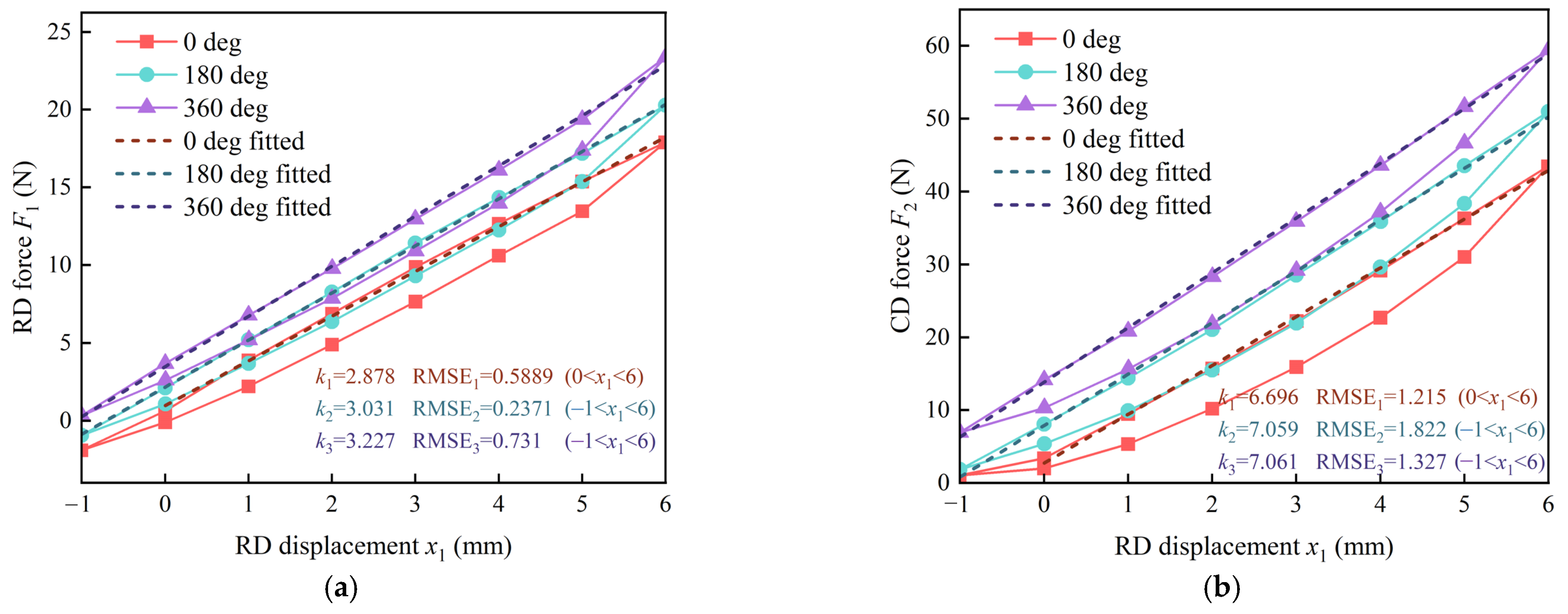
• The experiments with different diaphragm displacements show that the forces of the diaphragms increase with the increase in the RD displacement and decrease with the increase in the CD displacement. There is hysteresis in the axial reciprocating motion of the diaphragm, and the hysteresis decreases with the increase in the CD displacement.
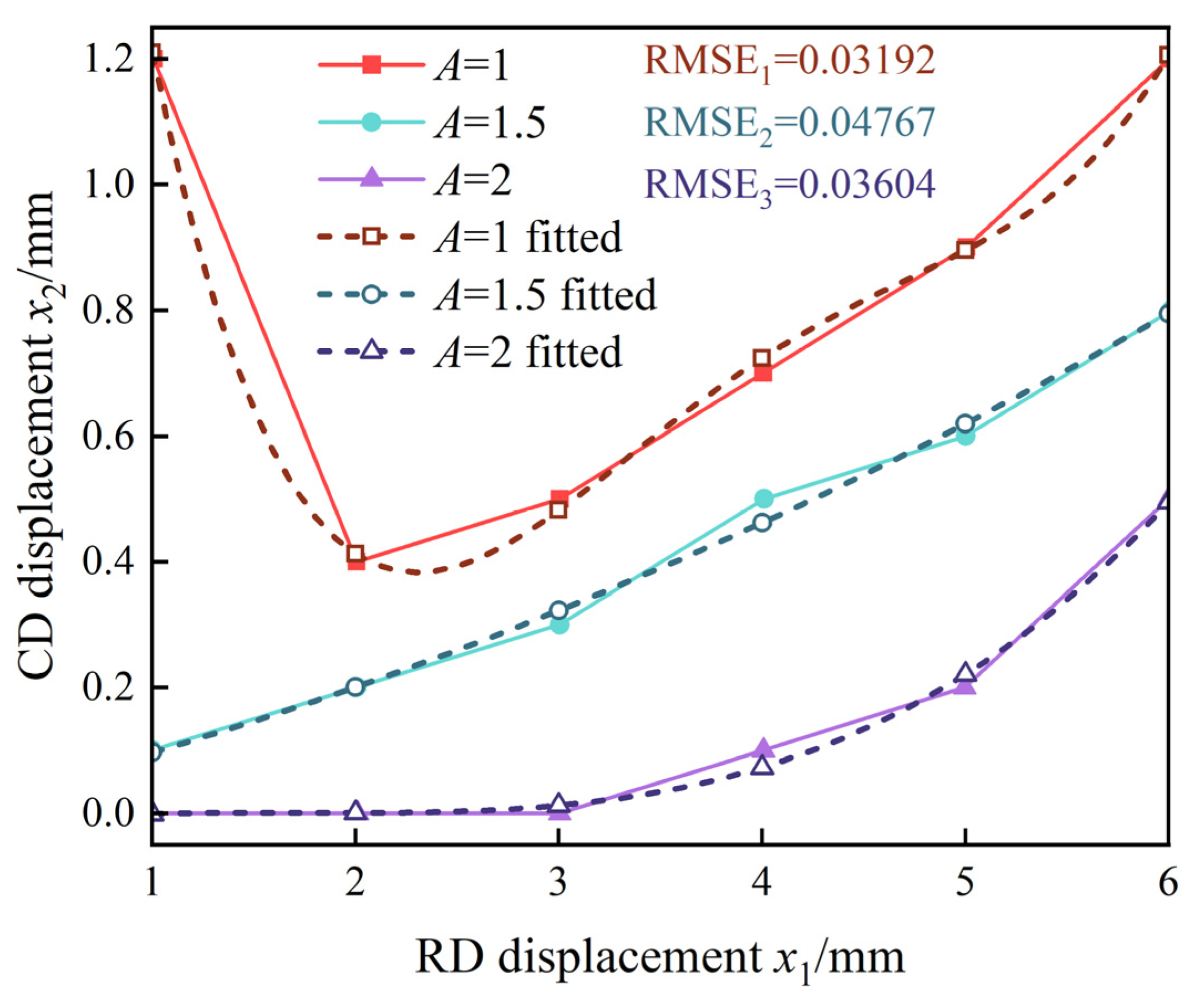
• The trend of the FARs with displacement shows that when the displacements of the RD exceed 2 mm, the FARs increase with the increase in the RD displacement but decrease with the increase in the CD displacement. The maximum FAR of the HFAM in the research is 2.5. Based on the FARs of 1, 1.5, and 2, the fitting expressions of the critical curves were obtained, and the displacement ranges of the RD and CD under different FAR ranges were determined.
• The experiments with different initial volumes show that when the displacements of the RD and the CD remain unchanged, the forces of the diaphragms increase with the increase in the initial volume. Furthermore, changing the initial volume does not affect the hysteresis of the diaphragms.
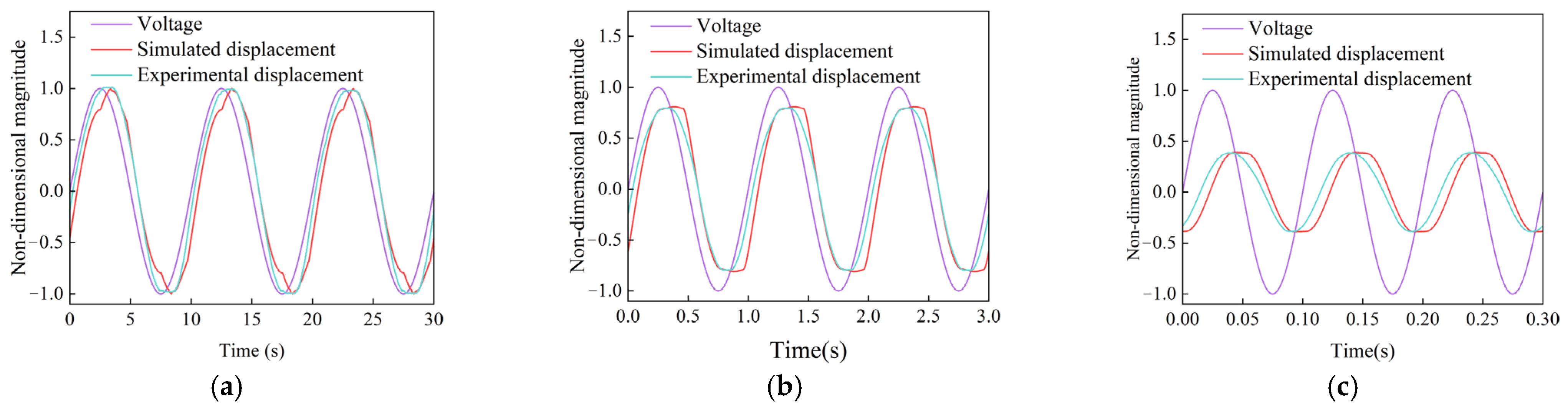
• Dynamic experiments show that when the frequency is less than 1 Hz, the maximum magnitude deviation between the simulation and the experiment is 0.35 dB, and the maximum phase deviation is 3.04 degrees. When the frequency is greater than 1 Hz, the maximum magnitude deviation between the simulation and the experiment is 1.14 dB, and the maximum phase deviation is 21.96 degrees. The accuracy of the established dynamic model was verified, and the model is helpful to the practical application of the HFAM.
• In subsequent research, factors such as temperature and pressure could be added to the model to further improve the accuracy of the model to adapt to different working conditions. And the influence of the diaphragm size parameters on the working effect of the HFAMs could be further studied. Based on the study results, the working effect of the HFAMs can be optimized by adjusting the diaphragms’ sizes when facing different working conditions and requirements.

References

1. Xu, B.; Shen, J.; Liu, S.; Su, Q.; Zhang, J. Research and development of electro-hydraulic control valves oriented to industry 4.0: A review. Chin. J. Mech. Eng. 2020, 33, 29. [Google Scholar] [CrossRef]
2. Zhang, Y.; Yan, P.; Zhang, Z. High precision tracking control of a servo gantry with dynamic friction compensation. ISA Trans. 2016, 62, 349–356. [Google Scholar] [CrossRef]
3. Xie, F.; Zhou, R.; Wang, D.; Ke, J.; Guo, X.; Nguyen, V.X. Simulation study on static and dynamic characteristics of electromagnet for electro-hydraulic proportional valve used in shock absorber. IEEE Access 2020, 8, 41870–41881. [Google Scholar] [CrossRef]
4. Kim, H.J.; Yang, W.S. Effect of asymmetric piezoelectric multimorph ceramic on frequency response characteristics of piezoelectric acoustic actuator. In Proceedings of the 2013 Joint IEEE International Symposium on Applications of Ferroelectric and Workshop on Piezoresponse Force Microscopy (ISAF/PFM), Prague, Czech Republic, 21–25 July 2013; IEEE: Piscataway Township, NJ, USA, 2013; pp. 332–335. [Google Scholar]
5. Gou, J.; Ma, T.; Liu, X.; Zhang, C.; Sun, L.; Sun, G.; Xia, W.; Ren, X. Large and sensitive magnetostriction in ferromagnetic composites with nanodispersive precipitates. NPG Asia Mater. 2021, 13, 6. [Google Scholar] [CrossRef]
6. Mohith, S.; Rao, M.; Karanth, N.; Kulkarni, S.M.; Upadhya, A.R. Development and assessment of large stroke piezo-hydraulic actuator for micro positioning applications. Precis. Eng. 2021, 67, 324–338. [Google Scholar]
7. Wang, B.; Xu, N.; Wu, P.; Yang, R. Simulation on an electro-hydrostatic actuator controlled by a high-pressure piezoelectric pump with a displacement amplifier. Assem. Autom. 2021, 41, 413–418. [Google Scholar] [CrossRef]
8. Xiao, R.; Shao, S.; Xu, M.; Jing, Z. Design and analysis of a novel piezo-actuated XYθz micropositioning mechanism with large travel and kinematic decoupling. Adv. Mater. Sci. Eng. 2019, 2019, 5461725. [Google Scholar] [CrossRef]
9. Song, E.Z.; Zhao, G.F.; Yao, C.; Ma, Z.K.; Ding, S.L.; Ma, X.Z. Study of nonlinear characteristics and model based control for proportional electromagnet. Math. Probl. Eng. 2018, 2018, 2549456. [Google Scholar] [CrossRef]
10. Kim, J.Y.; Ahn, D. Analysis of high force voice coil motors for magnetic levitation. Actuators 2020, 9, 133. [Google Scholar] [CrossRef]
11. Schmitt, P.; Hoffmann, M. Engineering a compliant mechanical amplifier for MEMS sensor applications. J. Microelectromech. Syst. 2020, 29, 214–227. [Google Scholar] [CrossRef]
12. Pan, B.; Zhao, H.; Zhao, C.; Zhang, P.; Hu, H. Nonlinear characteristics of compliant bridge-type displacement amplification mechanisms. Precis. Eng. 2019, 60, 246–256. [Google Scholar] [CrossRef]
13. Zhu, J.; Hao, G. Design and test of a compact compliant gripper using the Scott–Russell mechanism. Arch. Civ. Mech. Eng. 2020, 20, 81. [Google Scholar] [CrossRef]
14. Zhang, Y.; Li, D.; Chen, Y.; Zhang, B. Design of micro-displacement amplifier for the micro-channel cooling system in the micro-pump. Forsch. Im Ingenieurwesen Eng. Res. 2020, 84, 161–168. [Google Scholar] [CrossRef]
15. Ling, M.; Wang, J.; Wu, M.; Cao, L.; Fu, B. Design and modeling of an improved bridge-type compliant mechanism with its application for hydraulic piezo-valves. Sens. Actuators A Phys. 2021, 324, 112687. [Google Scholar] [CrossRef]
16. Tang, H.; Li, Y.; Xiao, X. Development and assessment of a novel hydraulic displacement amplifier for piezo-actuated large stroke precision positioning. In Proceedings of the 2013 IEEE International Conference on Robotics and Automation, Karlsruhe, Germany, 6–10 May 2013; IEEE: Piscataway Township, NJ, USA, 2013; pp. 1409–1414. [Google Scholar]
17. Muralidhara; Rao, R. Displacement characteristics of a piezoactuator-based prototype microactuator with a hydraulic displacement amplification system. J. Mech. Sci. Technol. 2015, 29, 4817–4822. [Google Scholar] [CrossRef]
18. Tian, X.C.; Wang, H.G.; Wang, H.; Wang, Z.C.; Sun, Y.Z.; Zhu, J.Z.; Zhao, J.; Zhang, S.; Yang, Z. Design and test of a piezoelectric micropump based on hydraulic amplification. AIP Adv. 2021, 11, 065230. [Google Scholar] [CrossRef]
19. Yang, Z.; He, Z.; Li, D.; Cui, X.; Xue, G.; Zhao, Z. Dynamic analysis and application of a novel hydraulic displacement amplifier based on flexible pistons for micro stage actuator. Sens. Actuators A Phys. 2015, 236, 228–246. [Google Scholar] [CrossRef]
20. Whitney, J.P.; Glisson, M.F.; Brockmeyer, E.L.; Hodgins, J.K. A low-friction passive fluid transmission and fluid-tendon soft actuator. In Proceedings of the 2014 IEEE/RSJ International Conference on Intelligent Robots and Systems, Chicago, IL, USA, 14–18 September 2014; IEEE: Piscataway Township, NJ, USA, 2014; pp. 2801–2808. [Google Scholar]
21. Liu, B.; Zheng, G.; Wang, A.; Gui, C.; Yu, H.; Shan, M.; Zhong, Z. Optical fiber Fabry–Perot acoustic sensors based on corrugated silver diaphragms. IEEE Trans. Instrum. Meas. 2019, 69, 3874–3881. [Google Scholar] [CrossRef]
22. Peng, X.; Han, L.; Li, L. A consistently compressible Mooney-Rivlin model for the vulcanized rubber based on the Penn’s experimental data. Polym. Eng. Sci. 2021, 61, 2287–2294. [Google Scholar] [CrossRef]
23. Meththananda, I.M.; Parker, S.; Patel, M.P.; Braden, M. The relationship between Shore hardness of elastomeric dental materials and Young’s modulus. Dent. Mater. 2009, 25, 956–959. [Google Scholar] [CrossRef]
24. Zhang, H.; Dong, J.; Cui, C.; Liu, S. Stress and strain analysis of spherical sealing cups of fluid-driven pipeline robot in dented oil and gas pipeline. Eng. Fail. Anal. 2020, 108, 104294. [Google Scholar] [CrossRef]
Figure 1. Flexible layout diagram of the HFAM: (a) the non-parallel force amplification transmission between the actuator and the load and (b) the orthogonal force amplification transmission between the actuator and the load.
Applsci 15 02754 g001
Figure 2. Structural diagram of the piezoelectric micropump [18].
Applsci 15 02754 g002
Figure 3. Structural diagram of the piezo hydraulic amplification mechanism [6].
Applsci 15 02754 g003
Figure 4. Structural diagram of the flexible piston hydraulic amplification mechanism.
Applsci 15 02754 g004
Figure 5. Working principle of the HFAM.
Applsci 15 02754 g005
Figure 6. Force state diagram of HFAM.
Applsci 15 02754 g006
Figure 7. Dynamic model of HFAM in Simulink.
Applsci 15 02754 g007
Figure 8. Solid model and grid model of finite element simulations: (a) solid model of RD; (b) solid model of CD; (c) grid model of RD; and (d) grid model of CD.
Applsci 15 02754 g008
Figure 9. Simulation results of the RD part model using the free triangle grid: (a) the displacement cloud diagram. (b) The stress cloud diagram.
Applsci 15 02754 g009
Figure 10. Quadrilateral grid of the RD part.
Applsci 15 02754 g010
Figure 11. Simulation results of the RD part model with the quadrilateral grid: (a) The displacement cloud diagram. (b) The stress cloud diagram.
Applsci 15 02754 g011
Figure 12. Displacement and stress cloud diagrams. (a) Displacement cloud diagram of the RD; (b) stress cloud diagram of the RD; (c) displacement cloud diagram of the CD; and (d) stress cloud diagram of the CD.
Applsci 15 02754 g012
Figure 13. Relationships between the displacement, volume, and force of the diaphragm. (a) The relationships between the displacement, volume, and force of the RD. (b) The relationships between the displacement, volume, and force of the CD.
Applsci 15 02754 g013
Figure 14. Experimental system diagram of HFAM.
Applsci 15 02754 g014
Figure 15. Experimental system physical diagram. (a) Static characteristics experimental system; (b) friction force measurement experimental system; and (c) dynamic characteristics experimental system.
Applsci 15 02754 g015aApplsci 15 02754 g015b
Figure 16. Experiments of different RD displacements. (a) RD mechanical characteristics of area 1; (b) CD mechanical characteristics of area 1; (c) RD mechanical characteristics of area 2; (d) CD mechanical characteristics of area 2; (e) RD mechanical characteristics of area 3; (f) CD mechanical characteristics of area 3; (g) RD mechanical characteristics of area 4; and (h) CD mechanical characteristics of area 4.
Applsci 15 02754 g016
Figure 17. Experiments of different CD displacements. (a) RD mechanical characteristics. (b) CD mechanical characteristics.
Applsci 15 02754 g017
Figure 18. FAR diagram of HFAM. (a) Three-dimensional diagram of FARs. (b) Two-dimensional diagram of FARs.
Applsci 15 02754 g018aApplsci 15 02754 g018b
Figure 19. Displacement ranges of diaphragms with different FARs.
Applsci 15 02754 g019
Figure 20. Different initial volume experiments. (a) RD mechanical characteristics. (b) CD mechanical characteristics.
Applsci 15 02754 g020
Figure 21. Dimensionless dynamic characteristics curves. (a) Dimensionless curves at 0.1 Hz; (b) dimensionless curves at 1 Hz; and (c) dimensionless curves at 10 Hz.
Applsci 15 02754 g021
Figure 22. HFAM system Bode diagram.
Applsci 15 02754 g022