Abstract
In this experimental work, sloshing tests were performed with containers filled with water at 50% of their volume capacity. Two boundary conditions were considered: uncoated containers and containers with hydrophobic coated walls. In addition, several aspect ratios (container width over length) were tested. We characterized two regimes, the first when the container is periodically forced at a frequency lower than its resonant frequency and the second after the forcing is suddenly stopped. In each case, the amplitude of the waves was measured. Several surprising results were found. First, in the forced regime, the sloshing amplitude was lower in the hydrophobic containers than in the containers with the non-hydrophobic walls, despite the free-slip condition in the former case. Second, the damping after sudden stoppage was much higher in the containers with hydrophobic walls than in the uncoated containers. This behavior is explained by the collision of waves with oil-coated walls, which generates a lower load pressure. Finally, we found that the damping depends on the dimension of the container through , and is greater when . These experimental findings open the way for further innovative research.
1. Introduction
The sloshing phenomenon generally occurs in partially filled tanks with accelerated movement, e.g., liquid cargo ships in non-fully loaded navigation, moving oil tank transporters, elevated water towers perturbed by ground motion, and road vehicle tanks [1,2]. Special applications include aerospace fuel tanks, the stability of which is very sensitive to uncontrolled oscillations [3]. This nonlinear phenomenon can lead to spillage of the transported liquid, or in the worst case damage to the container [4]. If the forcing lasts long enough, the sloshing intensity can cause significant compressive forces on the container walls and may be a source of destabilization or failure, especially if the forcing frequency is equal to the system’s natural frequency. Therefore, rapid stabilization or wave damping is crucial to avoiding disasters.
Several techniques have been developed to control sloshing and reduce the stresses on container walls. For example, through a series of controlled and detailed experiments, the work of [5] demonstrated the effectiveness of four different vertical baffle configurations to dampen the effects of sloshing and suppress the pressure on walls due to breaking waves. With the same purpose, Ref. [6] studied the effect of damping on the sloshing pressure under resonance conditions through numerical analysis by placing two baffles in a partially filled rectangular tank. Different heights and/or distances between the baffles were tested and provided good results. Following the same objective, Ref. [7] proposed a new configuration that consisted of placing a horizontal perforated plate inside a container, which significantly reduces the wave amplitude and controls the sloshing. In [8], the authors further improved this method by placing horizontal baffles of different length, porosity, and depth. They found that sloshing tended to decrease when porosity was increased, and that the energy loss was mainly due to eddies generated when the fluid passed through the pores.
Therefore, the effectiveness of energy dissipation by baffles in containers is clear. Moreover, it has been shown that the oscillation amplitude of the free surface depends on the viscosity. In [2], the authors found through experiments conducted in a 70% filled tank that higher liquid viscosity results in a greater reduction in sloshing pressure and splashing. They showed that for highly viscous fluids, friction with the container walls dissipates most of the energy. In addition, Ref. [9] used numerical and experimental modeling to demonstrate that for highly viscous liquids the energy is mainly dissipated by the wall boundary layers. Therefore, sloshing is significantly lower with glycerin than with water. Viscosity can also be used to dampen sloshing when used as a thin layer on the free surface of water. In this way, Ref. [10] performed experiments with two non-miscible liquid layers, that is, a layer of water in a partially filled reservoir covered by an upper layer of oil with a higher viscosity. When the depth of the water was 10 cm and the thickness of the oil layer was equal to 5 cm, the free surface was more stable than with a single layer of water, while when the upper layer was 2.5 cm deep it was more stable.
The ‘anti-sloshing’ technique proposed the use of floating liquid foams for the same purpose. A number of studies [11,12] have experimentally addressed the influence on sloshing of a liquid foam layer. Results have shown that a sufficiently thick foam layer (five layers of bubbles) increases the damping coefficient and reduces the amplitude of free-surface oscillations. Using an analytical model, the authors demonstrated that the dissipation of sloshing energy is mainly due to the bubbles closest to the walls. Based on the work of [12], the authors of [4] proposed placing solid spherical foams of uniform diameter on top of the fluid surface to minimize sloshing. Through a series of experiments, they demonstrated that the effect of one to four layers of solid foam proportionally reduced the amplitude of the natural frequency at the free surface of a rectangular tank. They concluded that the resulting energy dissipation of sloshing is due to friction between neighboring spheres.
The works mentioned above are only a small part of the vast literature available on techniques to minimize sloshing-induced loads; however, most existing research involves specialized engineering work that can be very costly, especially for large containers. Recently, Ref. [13] reported experiments performed in two identical containers under different conditions; in the first configuration the container was coated with a hydrophobic solution, while in the other it was left uncoated. They performed measurements using different modes of excitation related to the natural frequency of the tank and three different water levels (low, medium, and high). Their analysis was conducted for long excitation times. In the case of the intermediate level, the wall sloshing pressure load was reduced by up to , while no significant reduction was observed for the low and high levels. They concluded that hydrophobic surfaces lead to a reduction in load sloshing on the container walls along with reduced wave breaking.
Based on the results of [13], we present here an experimental study of sloshing in two configurations: with uncoated containers and with containers in which the walls are coated with hydrophobic oil. As described in Section 2, all containers were filled with water to the level, and eight different values for the aspect ratio of the containers were considered. We describe how video processing allows extraction of the water-free surface as a function of time. Moreover, the containers were subject to different two regimes: a periodically forced regime, leading to results reported in Section 3, and a damping regime after external forcing was suddenly stopped, leading to the results reported in Section 4. The main objective of the study was to compare the sloshing damping time of water in containers with hydrophobic and non-hydrophobic walls. Our results were compared with those from the work of [13]. Our conclusions and a corresponding discussion are provided in Section 6.
2. Experimental Procedure
2.1. Experimental Setup
The experiments were performed at the Geophysical Fluid Dynamics Laboratory of the University of Guadalajara, Mexico. Figure 1a shows a scheme of our experimental setup, which is similar to that used by [12]. It consists of two transparent acrylic containers with the same dimensions. The wall roughness is negligible, and of the lateral walls are perpendicular to the free surface of the water. The experimenter controlled their horizontal periodic motion through a DC motor. Both containers were on a moving stage on rails, and oscillated with a given amplitude and determined frequency f. Thus, their harmonic lateral movement is described by .
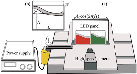
Figure 1.
(a) Schematic of the complete experimental setup, which is similar to that used by [12]. The platform slides on the rails with a minimum of friction; the rails are shown by the horizontal gray lines. Two containers with the same dimensions oscillate on the platform; the water in the uncoated container is dyed red, while the water in the container with hydrophobic walls is dyed green. The motor on the left allows the oscillation frequency to be fixed through the power supply. (b) Detailed view of the two containers along with their main parameters: water level H, container length L, container width W, and oscillation amplitude .
An LED panel was placed on the mobile platform behind the two containers to enhance visualization of the containers. In front of the containers, a high-speed camera fixed on the moving stage recorded the water’s superficial waves at 240 fps. Each container was partially filled with colored water. A green vegetable-based dye was used for the water in the hydrophobic-walled container and a red dye for the water in the non-hydrophobic container. All the walls of the first container, including its bottom, were coated with a thin layer of commercial Vaseline.
In order to illustrate the different hydrophobic/hydrophilic conditions of the containers, Figure 1a shows a drop of red-dyed water that was left on a flat dry acrylic surface, while Figure 1b shows an identical green-colored drop on the same acrylic surface previously coated with Vaseline. The contact angles [14] are pointed out in each of the photographs. The photographs clearly show that the apparent contact angle of the drop on the uncoated surface is greater than the angle of the drop on the Vaseline-coated surface, confirming the hydrophobicity of the green container.
The panel in Figure 2b points out the different parameters of our experiment: W is the width of the container, L is its length, H is the depth of water before forcing, and is the maximum/minimum level of the free surface concerning its equilibrium.

Figure 2.
Contact angles and of static drops of water placed on hydrophilic and hydrophobic surfaces. In (a), the drop is placed on a dry, solid, and flat surface without Vaseline, with . In (b), an identical drop is placed on a Vaseline-coated acrylic surface, with . The spatial scale is represented by the horizontal solid black line, which refers to the drop’s extension on the hydrophobic surface.
The free surface period and decaying time are controlled by the depth of the liquid H and the dimension of the container [15]. Measurements were made for eight different dimensions, each characterized by an aspect ratio . Table 1 shows the values for , W, L, and H used in our experiments. Moreover, the natural frequencies of the superficial were calculated using the following equation [16]:
where g is the acceleration of gravity. We confirmed the surface tension had no significant impact (lower than ) on the values.

Table 1.
Parameters of the eight configurations; is the containers’ aspect ratio, W and L are the width and length values, H is the liquid depth, and is the natural frequency determined by Equation (1).
The methodology was as follows. The oscillation amplitude of the container was maintained at a constant level equal to cm in all experiments. First, the DC motor was activated at a given low frequency. Videos were recorded during several oscillation periods, then the frequency was increased and the recording started again. The amplitude measurements are reported in Section 3.
After the forcing frequency of Hz was reached, the motor was suddenly stopped and the damping regime was recorded using the same video camera. The results of this process are shown in Section 4.
The present study was conducted using fresh water as the liquid. The viscosity, density, and surface tension of the water were considered to be constant, as our experiments were performed in the same laboratory which is maintained at a constant temperature of °C. Moreover, the containers were closed in the upper part using a cover.
2.2. Video Processing: Wave Height Estimation Based on RGB Images and Data Extraction
The water height at a given point was extracted from the videos using the following procedure. The frames were recorded in RGB format with a time step of 0.0042 s and spatial resolution of pixels. The physical dimensions of each pixel were estimated based on the distance between the free surface in equilibrium and the top of the same container, with a pixel corresponding to m. After each frame was extracted from the video, it was binarized with optimal noise filtering parameters. To eliminate spurious values obtained from the free surface video data, we used Matlab’s (R2023b) csaps function, which employs a cubic smoothing spline. Then, the time history of one column of the binarized matrix was plotted in a diagram, with the abscissa as the time and the y-axis as the space.
Figure 3 shows a frame in RGB format and the corresponding binarized version for the container with . The column of pixels that was extracted to characterize the free-surface history is indicated by the vertical red lines on the right.
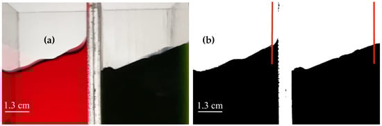
Figure 3.
(a) A particular frame of both containers in RGB bands for the container with and (b) the image binarization of the same frame. The column from which the data were extracted is indicated by the vertical red lines. Note the opacity of the container with hydrophobic walls (green color in (a)).
3. Forcing
As previously described, the excitation frequency was gradually increased over six values between 0 and Hz. Figure 4 shows the time history of the six signals for . The horizontal position of the container is indicated by the black line, where the maxima correspond to the position of the container on the right and are divided by for a better visualization. In the same graphics, the green and red curves show the water surface history for the containers with hydrophobic coating and no coating, respectively.
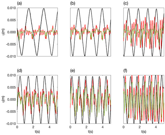
Figure 4.
Time history for the cells with . The external forcing is represented by the black line divided by , while the green and red lines indicate the water surface for the containers with hydrophobic coating on the walls and no coating, respectively. () Hz; () Hz; () Hz; () Hz; () Hz; () Hz.
These graphics point out that the water level oscillates with the same frequency as the forcing one but with several harmonics. As the system is excited with a frequency different from the natural one, this is to be expected. Moreover, as the forcing frequency f is higher, the oscillation amplitude of the water level is greater; this behavior is predictable since the system approaches its resonance. It is also important to note that for all the tested forcing frequencies, the oscillation amplitude is higher for the uncoated containers (red lines in Figure 4) than for the hydrophobic containers.
To quantify this difference, the left-hand vertical axis of Figure 5 shows the evolution of the amplitude as a function of the forcing frequency. The green bars are always lower than the red ones, as mentioned before. Now, the right-hand axis represents the difference in amplitude in % between the waves in the coated and uncoated containers. The solid blue line shows that the reduction in amplitude varies from for higher frequency values to for low frequency values, with an average value of approximately .
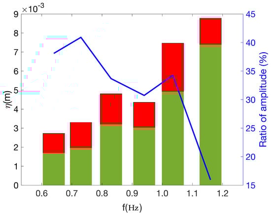
Figure 5.
Oscillation amplitude of the water level for as a function of the forcing frequency f (left-hand axis). Green bars: hydrophobic container walls; red bars: uncoated container walls. The blue solid line represents the ratio between both amplitudes in %, with an average of approximately .
It is interesting to note that our observations are different from the results reported by [13], who found an increment of the elevation of the free surface with hydrophobic walls. The resulting free-slip condition in the latter case should indeed promote faster motions of the water at the walls with higher waves. However, this was not the case in our experiments. This may be due to the development of a boundary layer despite the hydrophobic coating, as explained by [17]. Moreover, recent experiments have shown that greater friction coefficients can be generated by hydrophobic coated walls in comparison with hydrophilic coated walls [18].
4. Free Surface Damping
4.1. Damping Time
As mentioned above, the main objective of this work is to determine the influence of hydrophobic walls on the damping of the superficial waves after the container’s oscillation is suddenly stopped. Figure 6 shows the oscillations of the water level for both the uncoated container (red line) and the hydrophobic container (green line). It can be observed that the superficial waves in the container with hydrophobic walls are damped faster than the waves in the uncoated container. To quantify the damping time after the forcing was suddenly stopped, we used the following equation to fit the experimental points:
where corresponds to the initial amplitude and is the natural frequency of the superficial waves. To experimentally estimate the natural frequency of the superficial waves, the Fourier transform of the signal shown in Figure 6 was calculated. The spectrum for is shown in Figure 7.
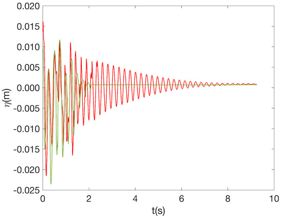
Figure 6.
Time history of the water level after periodic forcing was suddenly stopped for . The green line represents the container with hydrophobic coating and the red line represents the uncoated container.
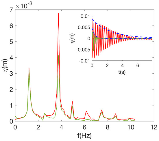
The first peak represents the external forcing frequency ( Hz) just before the excitation was stopped. The second peak corresponds to the natural frequency of the system ( Hz), which is consistent with Equation (1) and Table 1. The amplitude of the free surface waves in the uncoated container is observed to be greater than in the hydrophobic coated container by approximately .
The inset of Figure 7 shows an example of the evolution of the free surface elevation as a function of time for both containers after forcing was turned off. The dashed blue line is the external envelope of the damping process, i.e., , where and are two fitting parameters. The best fitted values were 2.50 Hz for the container with hydrophobic coating and 0.53 Hz for the container with uncoated walls. The higher value of for the hydrophobic container indicates greater damping. In this case with , the hydrophobic coating on the walls leads to about five times better dissipation of the superficial waves than in the uncoated container.
Applying the same process to all available containers (see Table 1), it is possible to estimate for the coated and uncoated configurations. Our results are reported in Figure 8 in the form of nondimensional parameters; the x-axis is , while the y-axis corresponds to . The latter quantity corresponds to the number of periods necessary for the system to be damped. The red curve is always above the green curve, which means that the uncoated containers require more time than the hydrophobic containers to attenuate the superficial waves.

Figure 8.
Damping values deduced from the best fits for each value presented in Table 1. Data points in green represent the hydrophobic containers, while those in red represent the uncoated ones.
It should be mentioned that an additional test was carried out on a pair of containers with larger dimensions of cm and cm, corresponding to an aspect ratio . It is interesting to note that the damping ratio was almost equal ( greater) compared to that reported for in Table 2. This result leads us to believe that is indeed the correct nondimensional parameter to consider.
Table 2.
Damping time for different values of . The relative difference is provided in %.
It is important to note that the less-damped uncoated container corresponds to , as more than eight periods are necessary to attenuate the waves. However, the effect of the hydrophobic walls is more efficient for the same container, as Table 2 shows that the highest damping effectiveness is reached for and . These results are discussed further in Section 5 below.
4.2. Waves Visualization
In this section, we describe a series of video snapshots of the tested hydrophobic and hydrophilic containers in order to compare them and discuss the influence of applying an oil-based coating to the walls.
Figure 9 shows six snapshots extracted from the video for 1 s after the forcing was suddenly stopped (see the inset of Figure 7). A time interval equal to 0.166 s separates each pair of images. Following the same methodology, the red color indicates hydrophilic walls and the green color hydrophobic ones. In panel (a), it can be observed that the red wave is slightly larger in amplitude and steeper than the green wave. However, the horizontal width is greater at the top of the green wave’s crest. This can be explained by greater adhesion of the fluid to the walls of the container under the hydrophilic condition. Note that both waves are in phase at this instant. In panel (b), the crests of the two waves again reach roughly the same amplitude on the opposite wall. The two waves also have roughly the same shape, although the green wave is again wider than the red one. The waves are still in phase. In panel (c), the waves are completely phase-shifted, and a shape similar to a breaking wave can be detected in the green container. Because of the hydrophobic wall in this container, the fluid cannot adhere to the wall; as a result, its shape is curved, which is contrary to the behavior of the fluid in the hydrophilic container. In panel (d), the waves are again phase-shifted, and an even greater difference in amplitude and shape is observed. In the red hydrophilic container, the waveform is now quite different from panel (a), with most of the liquid stuck to the wall. However, in the green hydrophopic container the wave is significantly attenuated. In panel (e), the wave in the hydrophilic container oscillates with the same amplitude as in panel (a), but now on the opposite wall, whereas the amplitude of the wave in the hydrophobic container continues to decrease. This suggests that the effect of the impact load on the walls is significantly reduced by the hydrophobic coating. Finally, the behavior of the two waves in panel (f) is similar to that in panel (e), except with a shifted phase.
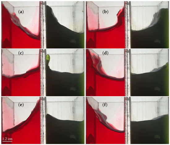
Figure 9.
Snapshots taken after forcing was suddenly stopped for . The fluid in the container with hydrophilic walls is dyed red, while the fluid in the container with hydrophobic coating is dyed green. There is a time difference of 0.166 s between each pair of images.
This behavior was found to be similar in all of our experiments, with the fluid adhering more readily to the uncoated walls of the hydrophilic container than to the walls with hydrophobic coating. The shape of the free surface in the latter container also remained smoother. These features show the importance of the boundary layer and hydrophobic effects, which appear as a source of energy dissipation.
4.3. Pressure Load
Although the fluid viscosity did not change in our experiments, the pressure loading on the walls of the containers did [13]. Because we could not directly measure the pressure on the vertical walls of the container, we estimated the pressure through the scaled absolute hydrostatic pressure of the wave [16]. This quantity was deduced from the wave elevation through the following expression:
Figure 10 shows three cycles of the pressure history for a portion of Figure 4b. In these graphics, the peaks correspond to the wave impact resulting from the external forcing on either lateral wall. For the first two peaks, the contact time is the same in the case of hydrophobic containers as in the hydrophilic ones. For the third peak, it is similar in amplitude but not time. The shape shows that it corresponds to a longer contact time for the green wave, resulting in greater energy loss despite similar pressure amplitude.

Figure 10.
Pressure–time history for two cycles with a given external forcing. The contact time with the wall for the green wave is pulse-like for the first two peaks, but not for the third peak.
5. Discussion
The higher damping in the case of hydrophobic walls is not intuitive, as the consequent nonslip condition should lead to lower dissipation in the boundary limit near the wall container. However, this result is in agreement with the results of [13], who measured the pressure load on the lateral walls for both uncoated containers and containers with a hydrophobic coating. They found that hydrophobicity caused a reduction in impact pressure, and consequently a decrease in sloshing effects. We found the same phenomenon here. In our work, quantitative measurements of the damping coefficient allow us to specify the reduction in sloshing due to the hydrophobic walls. Thus, our study complements the results of [13].
An important characteristic is that even though the waves are bidimensional, the damping coefficient depends on the width W through the aspect ratio , i.e., no dependence on the width direction was observed, as detailed in Section 4.2. However, it is well known that may depend on the width of the container W, as explained by [12,19], which is the case when a boundary layer develops on the lateral wall and causes dissipation due to the viscosity of the fluid. In the present case, the pressure load is exerted on the whole lateral wall.
Finally, although coating the walls of a container with Vaseline is not a convenient technique for reducing sloshing in real containers, as the Vaseline could mix with the transported liquid, use of hydrophobic adhesives [20,21] as a solution for sloshing reduction could be explored further. Moreover, our results on the influence of the aspect ratio could be studied more deeply through experiments performed with containers of the same length but with different widths, as in [22].
6. Conclusions
In this work, we have experimentally studied how applying a hydrophobic coating to the walls of a container can drastically dampen sloshing waves compared to an identical uncoated container. Previous work on sloshing damping has been performed both numerically [6,8,9,15] and experimentally [5,7,8,10,13]. Usually, sloshing damping is obtained through the installation of baffles inside the moving container; alternatively, different types of foam can be placed on the fluid surface for the same purpose [4,11,12]. In the present study, following the results of [13], we coated the walls of a container with a hydrophobic substance (Vaseline). We observed that when periodic external forcing was applied, the amplitude of the free surface in the container without the hydrophobic coating is always up to higher. In addition, we characterized the regime after forcing was suddenly stopped. In this case, we used an exponential function to fit the oscillation amplitude decrement through the damping time . This quantity was always lower for the container with the hydrophobic coating than for the uncoated container. This behavior is consistent with the observations of [13], who measured lower pressure loads when using a hydrophobic oil coating on the walls. We think that this result leads to interesting options for sloshing reduction through the application of hydrophobic adhesives to the internal walls of containers. Moreover, we found the value of to be strongly influenced by the container’s aspect ratio . For values of , the damping coefficient was reduced up to compared to the corresponding value for the uncoated container. Therefore, the energy loss due to interaction of the fluid with the hydrophobic walls together with the influence of the aspect ratio can provide a guideline for experiments performed through both numerical models and laboratory studies. Convenient container dimensions and hydrophobic wall coatings could also be combined with other techniques to reduce damping, such as baffles or foams.
Author Contributions
Conceptualization, R.C.C.-G. and A.C.; methodology, L.E.C.-P.; software, R.C.C.-G. and L.E.C.-P.; validation, C.O.M., R.C.C.-G. and A.C.; formal analysis, C.O.M.; investigation, R.C.C.-G.; resources, L.E.C.-P.; data curation, R.C.C.-G.; writing—original draft preparation, R.C.C.-G.; writing—review and editing, A.C and C.O.M.; visualization, R.C.C.-G.; supervision, C.O.M. All authors have read and agreed to the published version of the manuscript.
Funding
This research received no external funding.
Data Availability Statement
The raw data supporting the conclusions of this article will be made available by the authors on request.
Acknowledgments
The first author is grateful to the Geophysical Fluid Dynamics Laboratory and to the Fluid Mechanics Laboratory of CUCEI, Guadalajara University, for allowing us to perform the experiments. The authors gratefully acknowledge the comments of three anonymous reviewers for their careful reading and for providing very constructive comments that improved the paper.
Conflicts of Interest
The authors declare no conflicts of interest.
References
- Ibrahim, R.A. Liquid Sloshing Dynamics: Theory and Applications; Cambridge University Press: Cambridge, UK, 2005. [Google Scholar]
- Zou, C.F.; Wang, D.Y.; Cai, Z.H.; Li, Z. The effect of liquid viscosity on sloshing characteristics. Int. J. Nav. Archit. Ocean Eng. 2015, 7, 670–690. [Google Scholar] [CrossRef]
- Maleki, A.; Ziyaeifar, M. Sloshing damping in cylindrical liquid storage tanks with baffles. J. Sound Vib. 2007, 311, 372–385. [Google Scholar] [CrossRef]
- Zhang, C.; Su, P.; Ning, D. Hydrodynamic study of an anti-sloshing technique using floating foams. Ocean Eng. 2019, 175, 62–70. [Google Scholar] [CrossRef]
- Xue, M.A.; Zheng, J.; Lin, P.; Yuan, X. Experimental study on vertical baffles of different configurations in suppressing sloshing pressure. Ocean Eng. 2017, 136, 178–189. [Google Scholar] [CrossRef]
- Ma, C.; Xiong, C.; Ma, G. Numerical study on suppressing violent transient sloshing with single and double vertical baffles. Ocean Eng. 2021, 223, 108557. [Google Scholar] [CrossRef]
- Jin, H.; Liu, Y.; Li, H.J. Experimental study on sloshing in a tank with an inner horizontal perforated plate. Ocean Eng. 2014, 82, 75–84. [Google Scholar] [CrossRef]
- George, A.; Cho, I.H. Anti-slosh effect of a horizontal porous baffle in a swaying/rolling rectangular tank: Analytical and experimental approaches. Int. J. Nav. Archit. Ocean Eng. 2021, 13, 833–847. [Google Scholar] [CrossRef]
- Jin, X.; Lin, P. Viscous effects on liquid sloshing under external excitations. Ocean Eng. 2018, 171, 695–707. [Google Scholar] [CrossRef]
- Korkmaz, F.C. Damping of sloshing impact on bottom-layer fluid by adding a viscous top-layer fluid. Ocean Eng. 2022, 254, 111357. [Google Scholar] [CrossRef]
- Cappello, J.; Sauret, A.; Boulogne, F.; Dressaire, E.; Stone, H.A. Damping of liquid sloshing by foams: From everyday observations to liquid transport. J. Vis. 2015, 18, 269–271. [Google Scholar] [CrossRef][Green Version]
- Sauret, A.; Boulogne, F.; Cappello, J.; Dressaire, E.; Stone, H.A. Damping of liquid sloshing by foams. Phys. Fluids 2015, 27, 022103. [Google Scholar] [CrossRef]
- Korkmaz, F.C.; Güzel, B. Insights from sloshing experiments in a rectangular hydrophobic tank. Exp. Therm. Fluid Sci. 2023, 146, 110920. [Google Scholar] [CrossRef]
- Wang, Z.; Elimelech, M.; Lin, S. Environmental Applications of Interfacial Materials with Special Wettability. Environ. Sci. Technol. 2016, 50, 2132–2150. [Google Scholar] [CrossRef] [PubMed]
- Battaglia, L.; Cruchaga, M.; Storti, M.; D’Elía, J.; Núñez-Aedo, J.; Reinoso, R. Numerical modelling of 3D sloshing experiments in rectangular tanks. Appl. Math. Model. 2018, 59, 357–378. [Google Scholar] [CrossRef]
- Zou, C.F.; Wang, D.Y.; Cai, Z.H. Effects of boundary layer and liquid viscosity and compressible air on sloshing characteristics. Int. J. Nav. Archit. Ocean Eng. 2015, 7, 670–690. [Google Scholar] [CrossRef]
- Tretheway, D.C.; Meinhart, C.D. Apparent fluid slip at hydrophobic microchannel walls. Phys. Fluids 2002, 3, L9–L12. [Google Scholar] [CrossRef]
- Hansson, P.M.; Claesson, P.M.; Swerin, A.; Briscoe, W.H.; Schoelkopf, J.; Gane, P.A.; Thormann, E. Frictional forces between hydrophilic and hydrophobic particle coated nanostructured surfaces. Phys. Chem. Chem. Phys. 2013, 15, 17893–17902. [Google Scholar] [CrossRef]
- Bronfort, A.; Caps, H. Faraday instability at foam-water interface. Phys. Rev. E 2012, 86, 066313. [Google Scholar] [CrossRef]
- Wang, J.; He, L.; Pan, A.; Zhao, Y. Hydrophobic and durable adhesive coatings fabricated from fluorinated glycidyl copolymers grafted on SiO2 nanoparticles. ACS Appl. Nano Mater. 2018, 2, 617–626. [Google Scholar] [CrossRef]
- Tan, D.; Meng, F.; Ni, Y.; Sun, W.; Liu, Q.; Wang, X.; Shi, Z.; Zhao, Q.; Lei, Y.; Luan, S.; et al. Robust and smart underwater adhesion of hydrophobic hydrogel by phase change. Chem. Eng. J. 2023, 471, 144625. [Google Scholar] [CrossRef]
- Souto-Iglesias, A.; Bulian, G.; Botia-Vera, E. A set of canonical problems in sloshing. Part 2: Influence of tank width on impact pressure statistics in regular forced angular motion. Ocean Eng. 2015, 105, 136–159. [Google Scholar] [CrossRef]


Disclaimer/Publisher’s Note: The statements, opinions and data contained in all publications are solely those of the individual author(s) and contributor(s) and not of MDPI and/or the editor(s). MDPI and/or the editor(s) disclaim responsibility for any injury to people or property resulting from any ideas, methods, instructions or products referred to in the content. |
© 2025 by the authors. Licensee MDPI, Basel, Switzerland. This article is an open access article distributed under the terms and conditions of the Creative Commons Attribution (CC BY) license (https://creativecommons.org/licenses/by/4.0/).