Abstract
Traditional station passenger flow prediction can no longer meet the application needs of urban rail transit vehicle scheduling. Station passenger flow can only predict station distribution, and the passenger flow distribution in general sections is unknown. Accurate short-term travel origin and destination (OD) passenger flow prediction is the main basis for formulating urban rail transit operation organization plans. To simultaneously consider the spatiotemporal characteristics of passenger flow distribution and achieve high precision estimation of origin and destination (OD) passenger flow quickly, a predictive model based on a temporal convolutional network and a long short-term memory network (TCN–LSTM) combined with an attention mechanism was established to process passenger flow data in urban rail transit. Firstly, according to the passenger flow data of the urban rail transit section, the existing data characteristics were summarized, and the impact of external factors on section passenger flow was studied. Then, a temporal convolutional network and long short-term memory (TCN–LSTM) deep learning model based on an attention mechanism was constructed to predict interval passenger flow. The model combines some external factors such as time, date attributes, weather conditions, and air quality that affect passenger flow in the interval to improve the shortcomings of the original model in predicting origin and destination (OD) passenger flow. Taking Chongqing Rail Transit as an example, the model was validated, and the results showed that the deep learning model had significantly better prediction results than other baseline models. The applicability analysis in scenarios such as high/medium/low passenger flow could achieve stable prediction results.
1. Introduction
In today’s increasingly refined urban management, the timely and accurate prediction of rail transit passenger flow is a key component of urban rail transit construction plans. Urban rail transit operators can better understand the characteristics of and changes in urban rail transit passenger flow by processing the AFC (Auto Fare Collection) data of passengers. From the perspective of the development trend of passenger flow prediction in rail transit, traditional station entry and exit passenger flow prediction can no longer meet practical application needs. Because traditional station passenger flow prediction often focuses on predicting the total amount of passenger flow entering and leaving a certain station, it is difficult to distinguish the origin and destination (OD) of different passengers, and its guiding significance for urban rail transit transportation planning is limited [1]. Therefore, accurate prediction of origin and destination (OD) passenger flow is becoming a hot research topic for relevant scholars.
The main methods used by researchers to predict urban rail OD passenger flow can be divided into traditional methods, shallow machine learning methods, and deep learning methods. The more commonly used statistical origin–destination (OD) prediction methods in the early period are maximum entropy [2,3,4], maximum likelihood [5], least squares [6], and Bayesian inference [7]. Notably, the Kalman filter method stood out. Bhattacharjee et al. [8] first applied the Kalman filter method to the dynamic OD passenger flow prediction. Subsequently, time series models were also applied in OD prediction. Silva et al. [9] used an autoregressive model to process smart transport card data in London. For the predictive machine learning of OD passenger flow in London’s transit system, using a probability tree model, Leng et al. [10] learned from the historical OD information and obtained the probability of occurrence of each OD pair to predict destinations based on real-time starting point data and predict passenger flow in the metro network by accumulating all contributions. With the introduction of deep learning models into passenger flow prediction tasks, their neural network structure can better capture the spatiotemporal characteristics and variation patterns of data, thus achieving significant advantages in OD passenger flow prediction tasks [11]. In terms of a single model, Fu et al. [12] first used the GRU model to predict OD passenger flow in UTR passenger flow prediction. The results show that the GRU model is better than autoregressive synthetic moving average models. Ma et al. [13] reviewed the research status and application effects of a long short-term memory network (LSTM) on traffic flow prediction and summarized the optimization methods of the model in OD flow prediction. Zhang et al. [14] proposed a deep learning-based Generative Adversarial Network (GAN) for a more accurate prediction of short-term passenger flow in rail transit with higher efficiency and lower memory usage. Ye et al. [15] proposed an adaptive heterogeneous spatiotemporal graph convolution predictor to predict the amount of passenger data for short-term inter-station travel and dynamically adapt the spatiotemporal characteristics of OD traffic through a graph convolution neural network.
For the combination of multiple models, Wu et al. [16] modeled the spatial dependency of multiple stations in pairs and combined the Hypergraph Attention Recurrent Network (HGARN) and the Hawkes attention mechanism to simulate the impact of events and capture the key moments that affect passenger flow. Miao et al. [17] proposed an AEST model to improve OD prediction by solving the data coefficient problem of population flow in different areas of the city. Combining CNN/GCN and LSTM to effectively capture spatiotemporal correlations. Zou et al. [18] built a graph depth learning model (ST–GDL) for long-term OD prediction in view of the complex and dynamic spatiotemporal correlations of traffic information and also combined the extracted spatiotemporal features with meteorological information features to obtain more accurate prediction results. Wang et al. [19] combined a convolutional neural network (CNN) and a convolutional long short-term memory network (Conv–LSTM) to build an asymmetric spatiotemporal network (NTSN), which can predict bus OD by extracting spatiotemporal features, thus improving the generalization ability of NSTN.
In addition to the integration of models, the integration with attention mechanism is also a scheme to predict OD passenger flow. Lv et al. [20] proposed the PSAM-CNN model for the oversaturation of passengers in OD passenger flow prediction. The traditional CNN model combined with the attention mechanism of PSAM can accurately predict OD passenger flow when the urban subway is oversaturated. Zhang et al. [21] designed an adaptive graph convolution model based on self-attention to predict the future traffic demand between each pair of OD regions, taking the Encoder–Decoder structure as the historical input encoding as the hidden state and decoding it as the future prediction. At the same time, the combination with the self-attention mechanism can also capture the time dependence and improve the accuracy of the prediction. Liu et al. [22] designed an ST-MEN framework for dynamic spatial feature extraction to effectively capture the spatial dependency between OD passenger flow nodes, and they incorporated an external attention mechanism to effectively process external factors into the prediction process, thus achieving excellent prediction accuracy. Zeng et al. [23] constructed OD passenger flow stations as a matrix metro extension map and developed an SARGCN model integrating GCN, LSTM, and attention mechanisms to explore the spatiotemporal correlation between passenger inflow and outflow, and the model has excellent performance. Table 1 summarizes different passenger flow forecasting methods and the models used.

Table 1.
Summary of OD passenger flow related work.
In summary, current research on OD (origin–destination) passenger flow prediction is limited to data flow between stations, with a lack of focus on interval OD passenger flow prediction. Additionally, single models struggle to comprehensively capture the spatiotemporal features of interval OD passenger flows, while model integration requires considering the compatibility between models. To address these issues, our specific contributions are as follows:
- (1)
- A prediction model for interval OD passenger flow is proposed based on a core combination of TCN and LSTM, incorporating an attention mechanism to adaptively handle the data. The core components of this model can capture both the spatiotemporal features and long-term dependencies of the OD passenger flow data. The attention mechanism assigns weights to different time steps, helping the model focus on critical information, thus enabling the capture of more data features and improving the short-term prediction accuracy of urban-rail-transit interval OD passenger flows.
- (2)
- External factors related to interval OD passenger flow, such as date, time attributes, weather conditions, and air quality, are analyzed. The factors most strongly correlated with passenger flow are identified and incorporated into the model’s predictions, enhancing the model’s adaptability and generalization ability.
- (3)
- Using the urban rail transit system in the densely populated city of Chongqing as a case study, we validate the proposed model by conducting experiments on the city’s interval OD passenger flow. The model’s performance is tested under high-, medium-, and low-passenger-flow scenarios. The results demonstrate that the proposed model fits the actual variation trends of passenger flow more effectively, with the smallest prediction error under high-passenger-flow conditions. The findings are of significant relevance for future urban rail transit construction and daily operations.
2. Characteristics and Influencing Factors of Urban Rail Transit Passenger Flow
2.1. Dataset Source
The passenger flow data come from the Chongqing Rail Transit Group and are based on the card swiping data of passenger flow between Sigongli and Longtousi of Chongqing Rail Transit Line 3. The rail transit lines in the study area are shown in Figure 1, covering the entire city center area. The passenger flow data of Chongqing Rail Transit include the operation period of 6:00–24:00, and the passenger flow is divided into one-hour time granularity. The weather data corresponding to the actual travel time of passenger flow data can be queried through the national meteorological science data platform, including weather conditions, minimum temperature, maximum temperature, relative humidity, air quality, and other basic weather indicators. The weather properties are coded with Code 1 for sunny, Code 2 for cloudy, Code 3 for overcast, and Code 4 for rainy. Then, the time data are converted into floating-point data, and the two types of data are processed. The weather data are matched with the passenger flow data, and the passenger flow data are fused with the weather data to form a dataset.
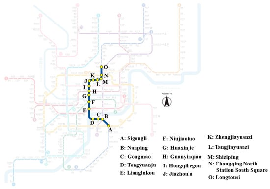
Figure 1.
Chongqing Rail Transit route map in China (research route highlighted).
2.2. OD Passenger Flow Characteristics
When passengers choose to travel by urban rail transit, the number of travel stations is mostly concentrated within a certain range. Based on the OD passenger flow distribution of Chongqing Metro Line 3, the 15 stations with the most concentrated passenger flow are selected and analyzed from Sigongli to Longtousi as representatives. Table 2 shows the interval passenger flow statistics of these 15 stations as of 1 May 2023. The letters A–O, respectively, represent 15 stations, including Sigongli, Nanping, Gongmao, Tongyuanju, Lianglukou, Niujiaotuo, Huaxinjie, Guanyinqiao, Hongqihegou, Jiazhoulu, Zhengjiayuanzi, Tangjiayuanzi, Shiziping, Chongqing North Station South Square, and Longtousi.
Table 2.
OD matrix of passenger flow.
Using the K-Means clustering method [24] to classify all OD passenger flow intervals, the clustering analysis is carried out to determine the classification standards for passenger flow at different stations, providing guidance for subsequent passenger flow prediction. The clustering results of the K-Means algorithm on the interval passenger flow data are shown in Figure 2. The asterisk is the cluster center, with the horizontal axis indicating the frequency of data points between stations and the vertical axis representing the corresponding passenger flow. The effective division of data is achieved by determining the central position of each category. From the figure, it can be observed that the 210 OD passenger flow intervals are divided into three categories, defined as high, medium, and low OD passenger flow intervals. The corresponding division results are shown in Table 3.
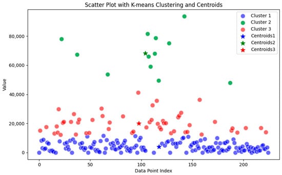
Figure 2.
Cluster results after execution of K-Means algorithm.
Table 3.
High, medium, and low OD passenger flow.
2.3. Analysis of Factors Affecting Passenger Flows
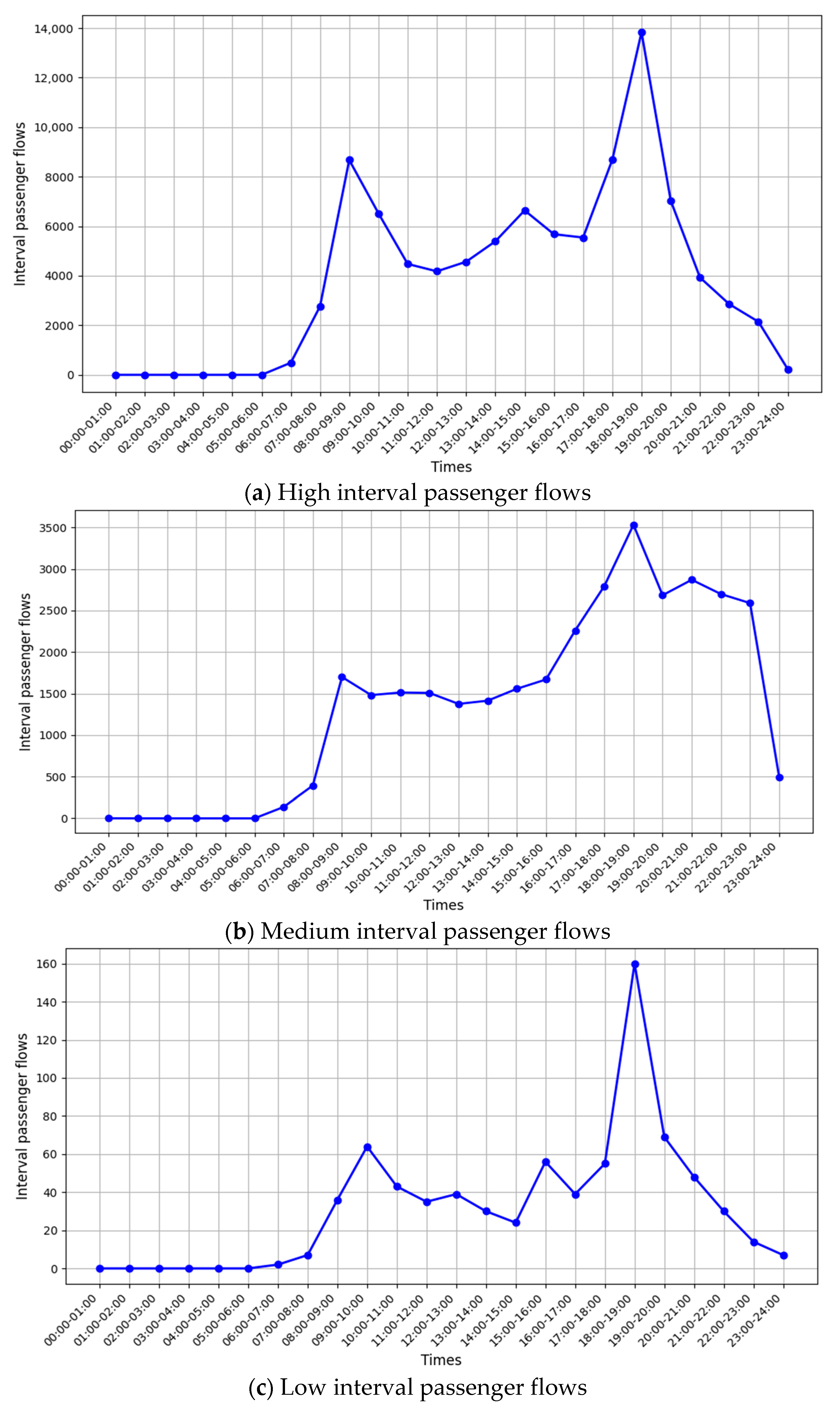
The change in interval passenger flow in urban rail transit has a certain time law. From the time attribute of the interval passenger flow data, it can be found that the passenger flow is constantly changing during the operation time of the rail transit in a day. In order to analyze the changing patterns of passenger flow over time during a certain period of time, three typical OD passenger flow sections were selected for analysis, from Jiazhoulu to Guanyinqiao (high interval passenger flows), Guanyinqiao to Huaxinjie (medium interval passenger flows), and Chongqing North Station South Square to Tongyuanju (low interval passenger flows). The passenger flow characteristics of the section on May 1st are shown in Figure 3.
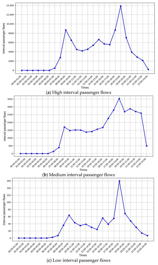
Figure 3.
Typical OD passenger flow statistics at different times.
For these three typical intervals, it can be seen that the peak passenger flow is mostly concentrated between 8:00–9:00 am and 18:00–19:00 pm during the 18 time intervals of Line 3 in a day. The distribution types of interval passenger flow in a day can be divided into five types: single peak, double peak, full peak, convex peak, and no peak [25]. The double peak refers to urban rail transit that forms an early peak due to commuting from 7:00 to 9:00 am and an evening peak due to work from 15:00 to 19:00 pm. The passenger flow data at other times do not change much and belong to the flat peak of passenger flow. According to the results, it can be found that the peak passenger flow in these three typical intervals belongs to double-peak passenger flow. When the other intervals are verified, it is found that basically all the peaks of the day are double peaks, with approximate times around 8:00–9:00 am and 18:00–19:00 pm.
In addition to time factors, weather may also have an impact on the OD passenger flow. Weather factors can affect passengers’ choice of other modes of transportation, leading to an increase or decrease in passenger flow. To achieve an accurate prediction of short-term OD passenger flow of urban rail transit, it is necessary to extract accurate feature factors. This study considers adding external weather factors to the model input. To verify whether there is a regular trend of weather-related interval passenger flow, the correlation of Pearson coefficient and Spearman coefficient in three typical intervals is analyzed: Jiazhoulu to Guanyinqiao (high interval passenger flows), Guanyinqiao to Huaxinjie (medium interval passenger flows), and Chongqing North Station South Square to Tongyuanju (low interval passenger flows). The characteristics of date attributes and time attributes are also analyzed for correlation, and finally, their significance is tested. The Pearson coefficient determines whether there is a linear correlation between the two variables [26], and the Spearman coefficient is used to measure whether there is a monotonic correlation between the two variables [27].
The larger the absolute value of the calculated Pearson correlation coefficient, the stronger the correlation. The Pearson correlation coefficient calculated for different influencing factors is shown in Table 4.
Table 4.
Pearson correlation coefficient affecting passenger flow.
The Spearman coefficient also has a value between −1 and 1, indicating that one of the two variables changes with the other over time. The Spearman coefficient calculated for different influencing factors is shown in Table 5.
Table 5.
Spearman correlation coefficient affecting passenger flow.
The p-value represents the probability of observing the current Pearson correlation coefficient and Spearman correlation coefficient under the premise that there is no linear correlation between the passenger flow in the interval and the relevant influencing factors. The value is calculated using a t distribution on the basis of the obtained correlation coefficients [28].
From the calculation results, for the Pearson coefficient, the minimum temperature, maximum temperature, weather conditions, and relative humidity are weakly correlated with the OD passenger flow, while the date attribute, time granularity, and air quality have a good linear correlation with the OD passenger flow. For the Spearman coefficient, only the date attribute is strongly correlated, while other influencing factors are weakly correlated. After comprehensively considering the correlation obtained from the two calculation methods, the date attribute, time granularity, air quality, and hourly passenger flow are used as parameter indicators for short-term OD passenger flow analysis and prediction, as shown in Table 6.
Table 6.
Influential parameters of passenger flow analysis prediction.
3. Construction of OD Passenger Flow Prediction Deep Learning Model
3.1. Temporal Convolutional Network Model
A temporal convolutional network (TCN) utilizes convolutional operations to capture local dependencies in a sequence and construct a deep network structure by stacking multiple convolutional layers, which provides a new method of hierarchical capture of space and time. The time convolutional network model has three main characteristics:
- (1)
- TCN uses causal convolution. Since each prediction can only rely on previous data predictions, there will be no data leakage. The principle of causal convolution is shown in Figure 4. The value of the previous layer at time t only depends on the value before the next layer at time t; thus, causal convolution cannot predict future values. Causal convolution has a unidirectional structure and strict constraints on timing, and too many convolutional layers will lead to gradient disappearance and a poor fitting effect.
- (2)
- TCN combines deep neural networks with dilated convolutions to form a model that can save long-term valid historical data. It can effectively improve the performance of the model and solve the problems of causal convolution. Expanding convolution mainly allows the filter to be applied to filer regions exceeding its own length range by ignoring some inputs, which is equivalent to adding zero to obtain a larger filter from the initial filter. The principle of the expanding structure is shown in Figure 5.
- (3)
- The TCN model introduces a residual network to build long-term dependencies, thereby effectively improving the model’s performance. The structure principle of the residual network is shown in Figure 6. To some extent, the residual connection overcomes the problems caused by the disappearance of local gradients and edge gradient explosions in convolutional neural networks to achieve cross-layer information input.
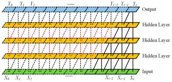
Figure 4.
Causal convolutional structure.
Figure 4.
Causal convolutional structure.
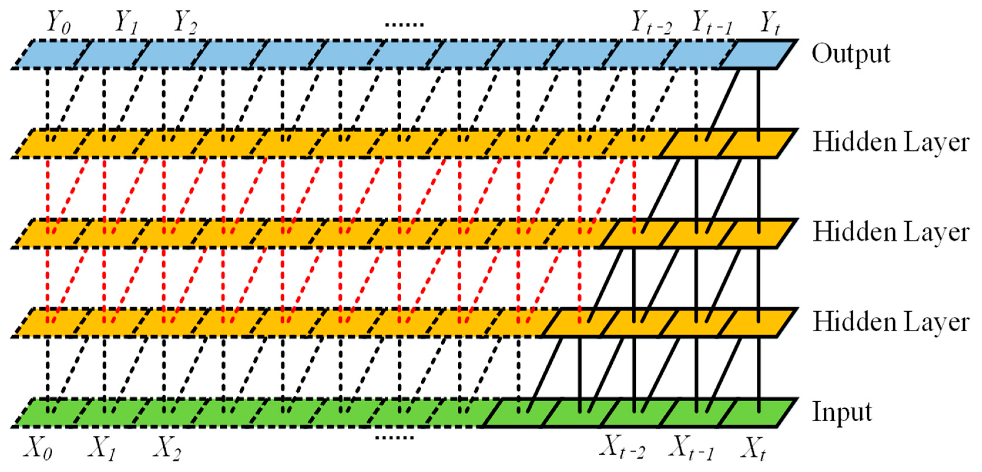
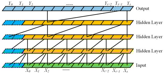
Figure 5.
Dilated convolutions.
Figure 5.
Dilated convolutions.
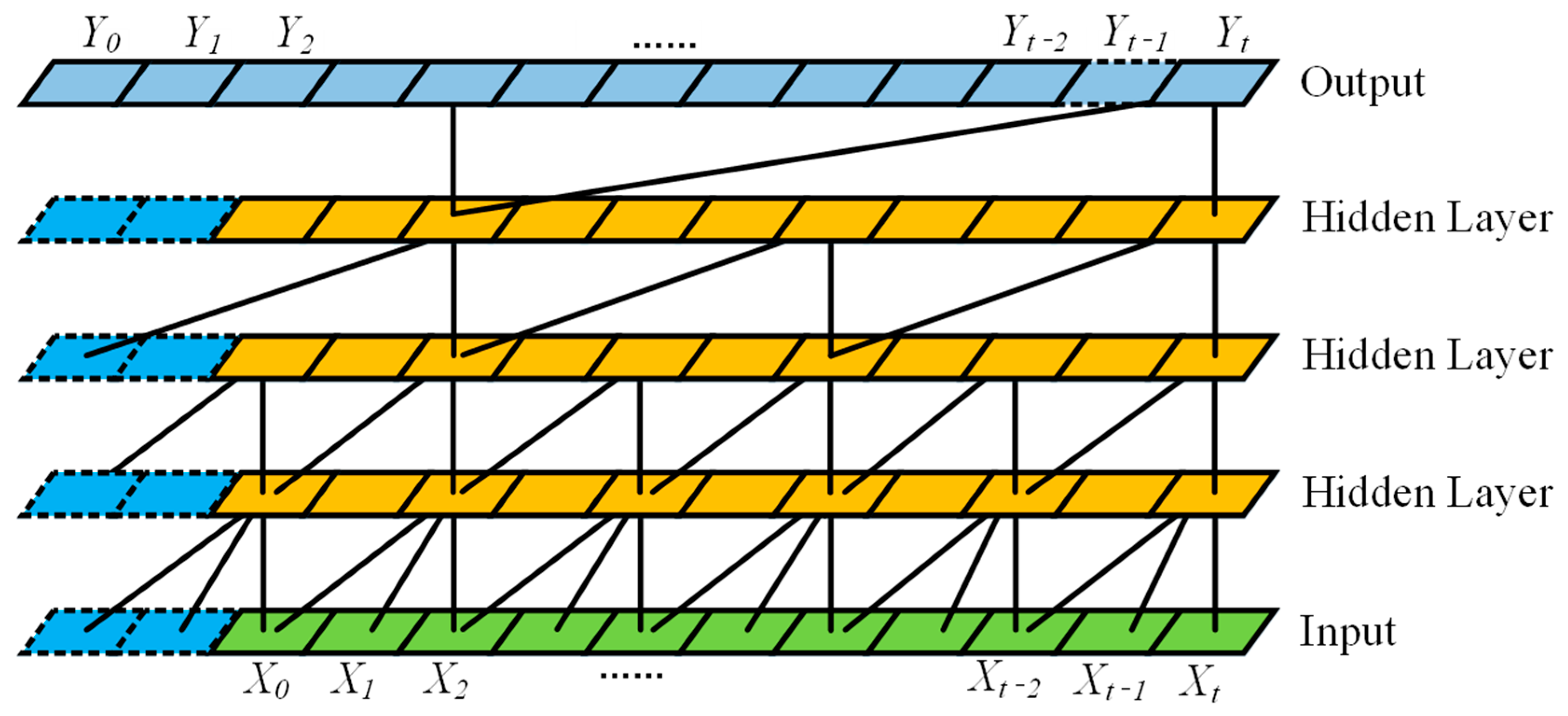
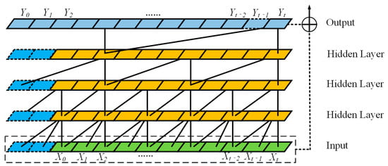
Figure 6.
Dilated convolutions with residual connection.
Figure 6.
Dilated convolutions with residual connection.
3.2. Long Short-Term Memory Network Model
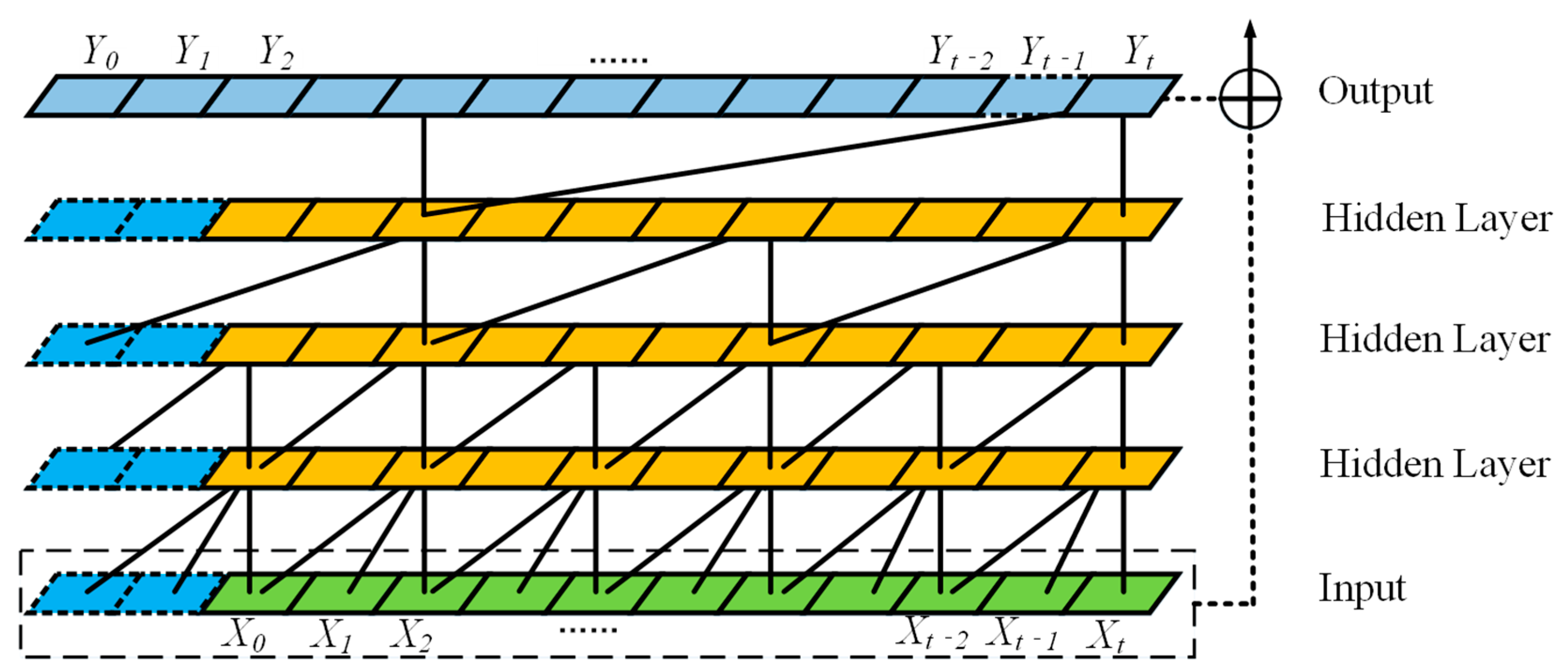
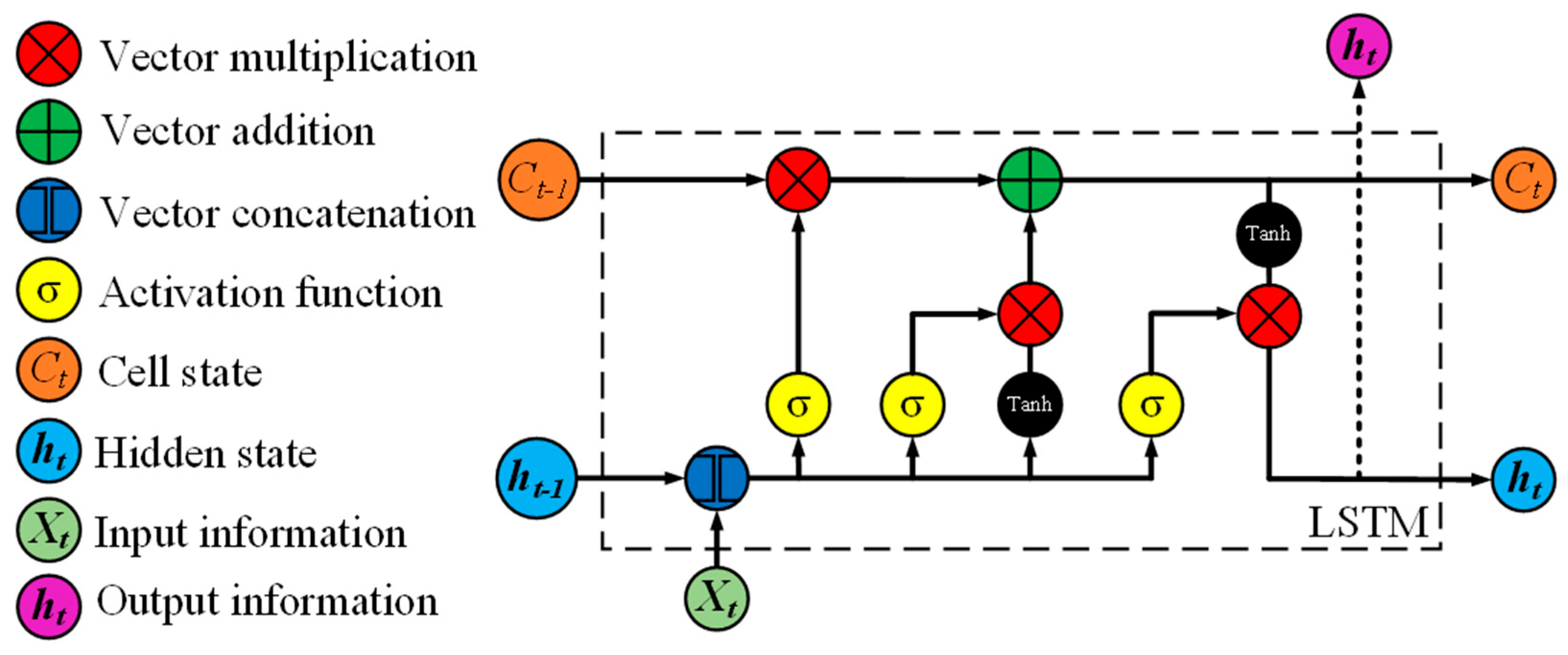
Long short-term memory (LSTM) is a variant of the Recurrent Neural Network (RNN). Compared with the RNN, the gradient disappearance can only be short-term memory through the gating mechanism; that is, LSTM introduces three gate structures: forget gate, input gate, and output gate in the RNN. An LSTM network combines short-term memory and long-term memory to learn long-term dependence in input data, and its structure is shown in Figure 7.
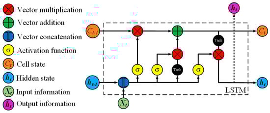
Figure 7.
LSTM model structure.
In the LSTM network, the activation function of the forget gate, input gate, and output gate is the Sigmoid function, and the activation function of the model output is the Tanh function. The expressions of these two functions and the corresponding derivative are calculated as follows:
The training process of the LSTM model can be roughly divided into the following four steps:
Step 1: After the input data at time t are input into the LSTM model, the forget gate begins to decide whether to discard the old data from the unit state at the previous moment. This step is calculated as follows:
where is the weight matrix of the forget gate, which combines with vectors and to obtain a new vector group , and the bias term of the forgetting gate is denoted by .
Step 2: The input gate determines how much data can be saved in the unit state Ct at time . During this process, it is possible to prepare and retain the necessary data, removing irrelevant data. This step is calculated as follows:
where is the weight matrix of the input gate, and is the corresponding bias term.
Step 3: Then, the tanh function is used to generate the candidate value of the unit state Ct corresponding to t at Ct. This step is calculated as follows:
In this process, and in the above equation are used to calculate the corresponding candidate states. Combining Step 1 and Step 2, the unit state of the previous moment is updated, the Sigmoid function is used to select the content that needs to be updated, and the tanh function is used to update the candidate states. The symbol ° indicates multiplication by the corresponding element. Step 3 is calculated as follows:
Step 4: The output gate determines the output value at the current time. This relationship is expressed as follows:
and are the weight matrix and bias term of the output gate, respectively, and the hidden layer state at time t is related to the cell state. This process is calculated as follows:
3.3. Attention Mechanism
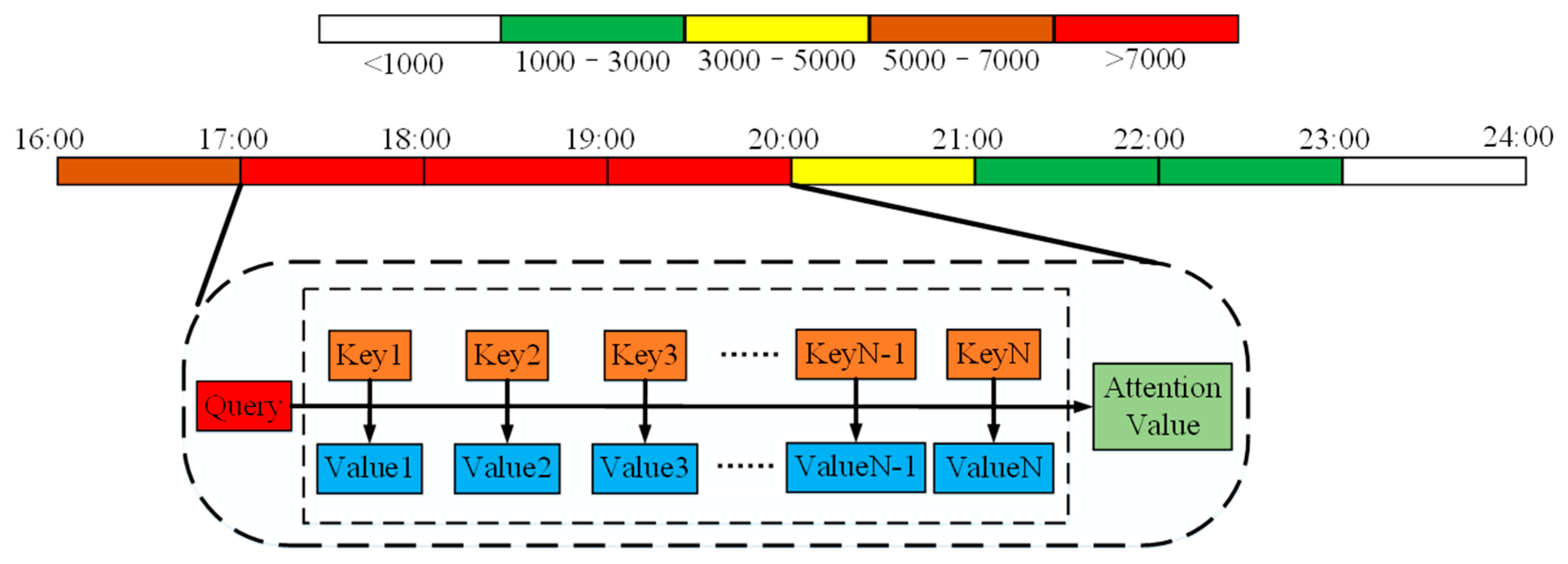
This study draws on the principle of attention mechanisms in the existing literature, and through the innovative adjustment of the overall architecture, the mechanism can be specialized for OD (starting and ending points) passenger flow prediction tasks. By assigning different weights to each influencing factor, we effectively improved the accuracy of the interval flow prediction, thus enhancing the accuracy and robustness of the prediction model. The specific form is shown in Figure 8. Assuming that the constituent elements in a data source (source) is composed of a series of <key, value> data pairs, given the query of a certain element in the target, the similarity or correlation between the query and each key is calculated to obtain the weight coefficient of the value corresponding to each key. Then, the value is weighted and summed to obtain the final attention value. Essentially, the attention mechanism is to weighted sum the values of elements in the data source (source), and query and key are used to calculate the weight coefficients of the corresponding values. By utilizing attention mechanisms, the model can better focus on the information of customer traffic and assign sufficient weight to key information. The passenger flow during peak hours is processed through the attention mechanism, and the processing process is as follows:
where Lx is the length of the data series.
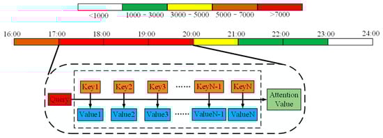
Figure 8.
The essence of the attention mechanism.
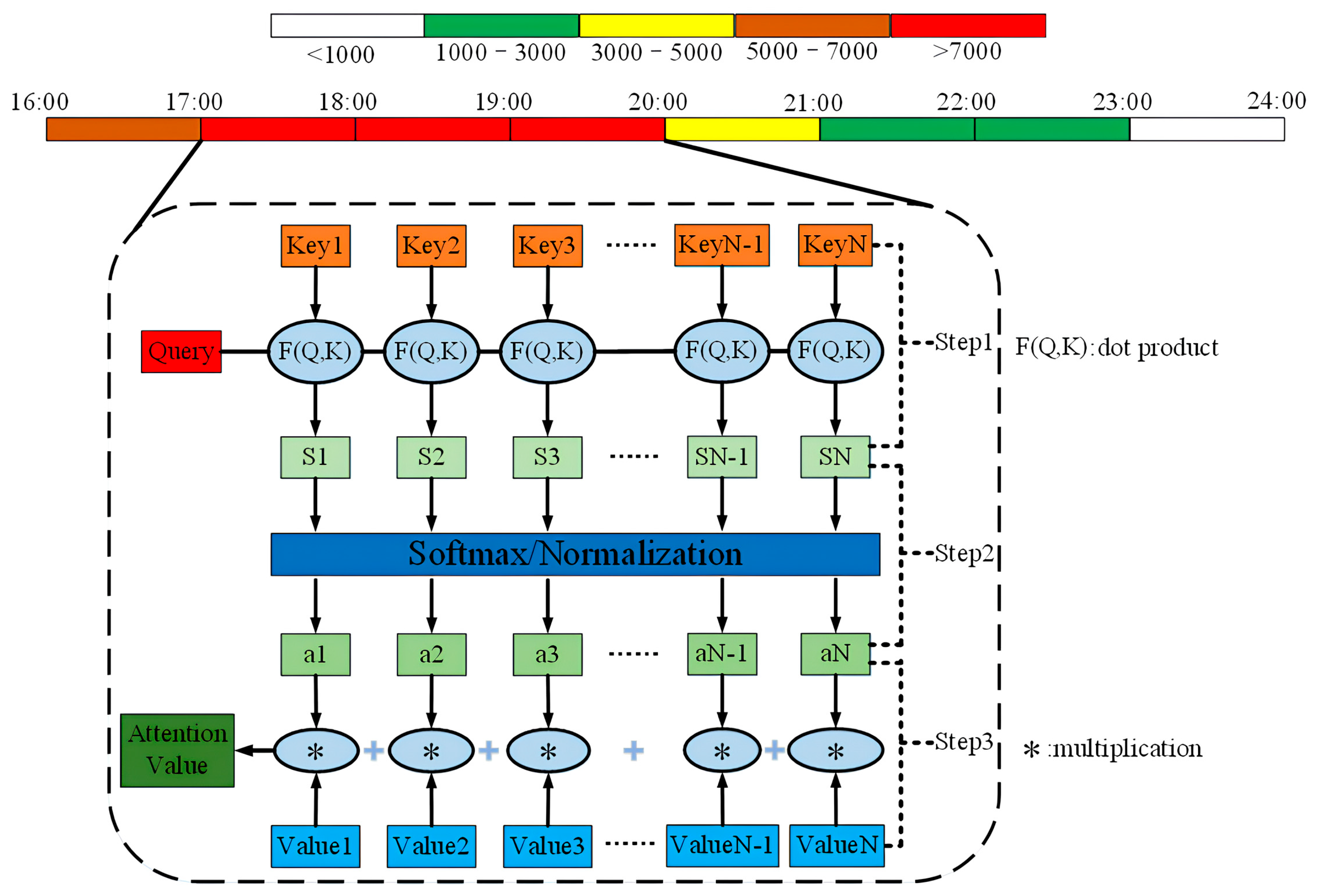
The calculation process of the attention mechanism can be roughly divided into three stages, as shown in Figure 9.
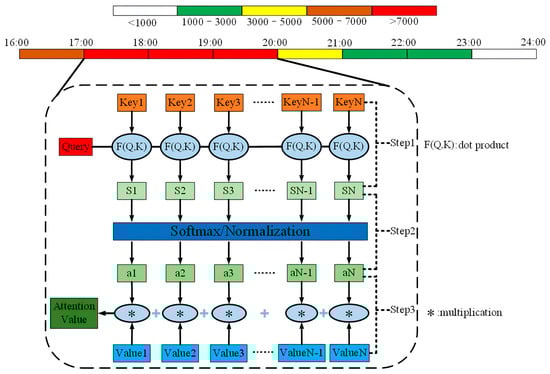
Figure 9.
Attention calculation process.
Step 1: According to the similarity or correlation between query and key calculations, the method used is a vector dot product calculation:
Step 2: The original score of the first stage is normalized. The original calculation branch is sorted into a probability distribution with the sum of all element weights of 1, and the weight of important elements is highlighted more through the internal mechanism of Softmax. It is calculated as follows:
Step 3: The weighted sum of the value term with the absolute weight coefficient is calculated as follows:
3.4. TCN–Attention–LSTM Model
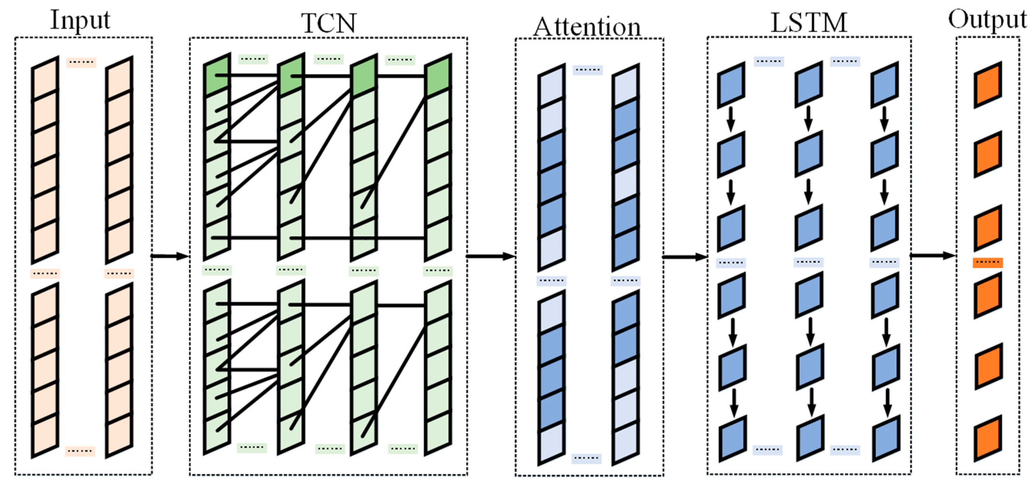
The OD passenger flow of urban rail transit gathers at various stations, which has a strong correlation with the spatial dimension of the stations, leading to mutual influence of OD passenger flow within a certain spatial range. At the same time, OD passenger flow exhibits certain periodic changes in the time dimension, such as the tidal pattern of morning and evening peak OD passenger flow analyzed earlier, which also includes a short-term autocorrelation of OD passenger flow, such as the short-term OD passenger flow changes caused by sudden changes in preceding passenger flow. Therefore, it is necessary to capture all features of OD passenger flow data through a combination model, considering the short-term autocorrelation and long-term periodicity of passenger flow demand. A temporal convolutional network (TCN) model and long short-term memory (LSTM) were used as the core, and an attention mechanism was introduced to construct a TCN–Attention–LSTM model for predicting the OD passenger flow of urban rail transit.
The model structure is shown in Figure 10. The processed OD passenger flow dataset is selected for data extraction, which is first normalized, and then the TCN is used to extract the features of the OD passenger flow data and time data. After that, the output data are sent to the attention layer. When the attention mechanism layer further extracts the features, the output of the attention mechanism layer is used as the input vector of the LSTM for training. In this way, the change law of the OD passenger flow is captured, and the prediction results are obtained.
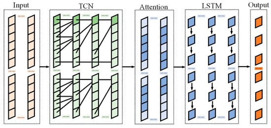
Figure 10.
Structure diagram of TCN-LSTM model.
4. Passenger Flow Prediction Results and Discussion
4.1. Experimental Design
In the TCN-LSTM model with an attention mechanism developed in this study, the TCN module has three residual blocks. The first residual block has 32 filters, a convolution kernel size of 3, and an expansion coefficient of 1. The second residual block has 32 filters, 3 convolution kernels, and 4 expansion coefficients. There are three layers in the LSTM module, and each layer sets the parameters of the hidden layer to 128. The number of neurons in the Dense layer is set to 1, and the output is one-dimensional data. The model training number is set to 300 times to follow the new weight; the time step is set to 32, and other parameters remain unchanged.
Based on the data proposed by the Chongqing Rail Transit Group, the first 80% of the data were used as the training set for model training, and the remaining 20% of the data were used as the testing set to verify the accuracy and effectiveness of the model prediction. The platform for the experimental model is Python 3.10, and third-party libraries such as Scikit learn, Keras, and TensorFlow were built in this environment to construct a short-term passenger flow prediction model.
4.2. Prediction Results and Analysis of OD Passenger Flow
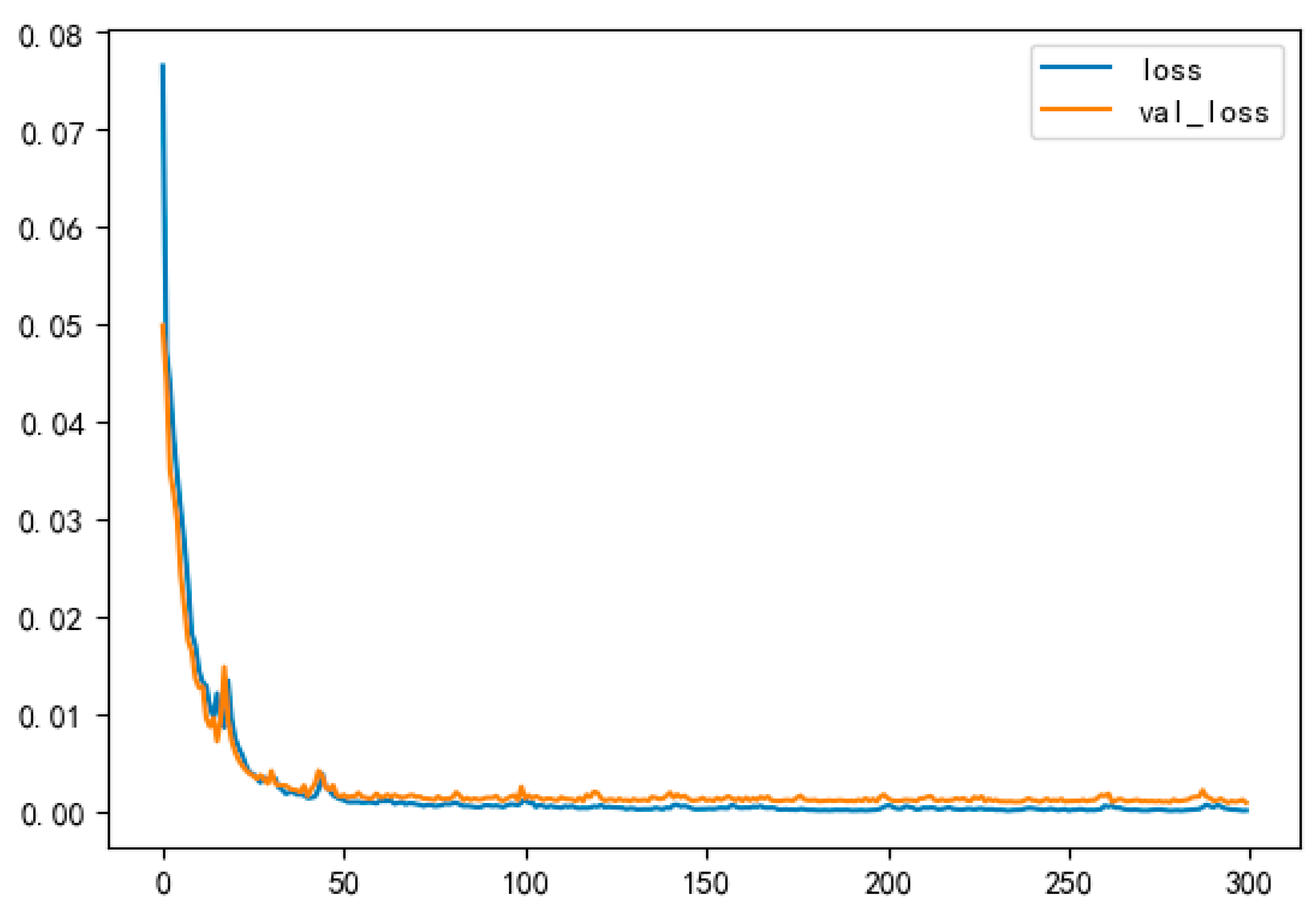
We conducted experiments using the OD passenger flow dataset of Chongqing Rail Transit. Firstly, the attention mechanism adaptively assigns different weights to different parts of the input data sequence. Then, the TCN–Attention–LSTM model is used to train and predict passenger flow data and generate prediction results. The goodness of fit and residual analysis of the model were evaluated through simulation experiments on three typical passenger flow intervals. Figure 11 shows the simulated loss value curve; the horizontal axis represents the number of training iterations, and the vertical axis is the training loss value. It can be seen that the two curves gradually become stable with the training of the model, which indicates that the training network runs normally.
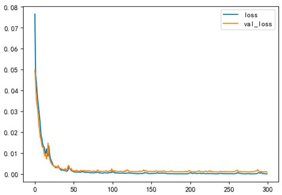
Figure 11.
Schematic diagram of combined model loss values.
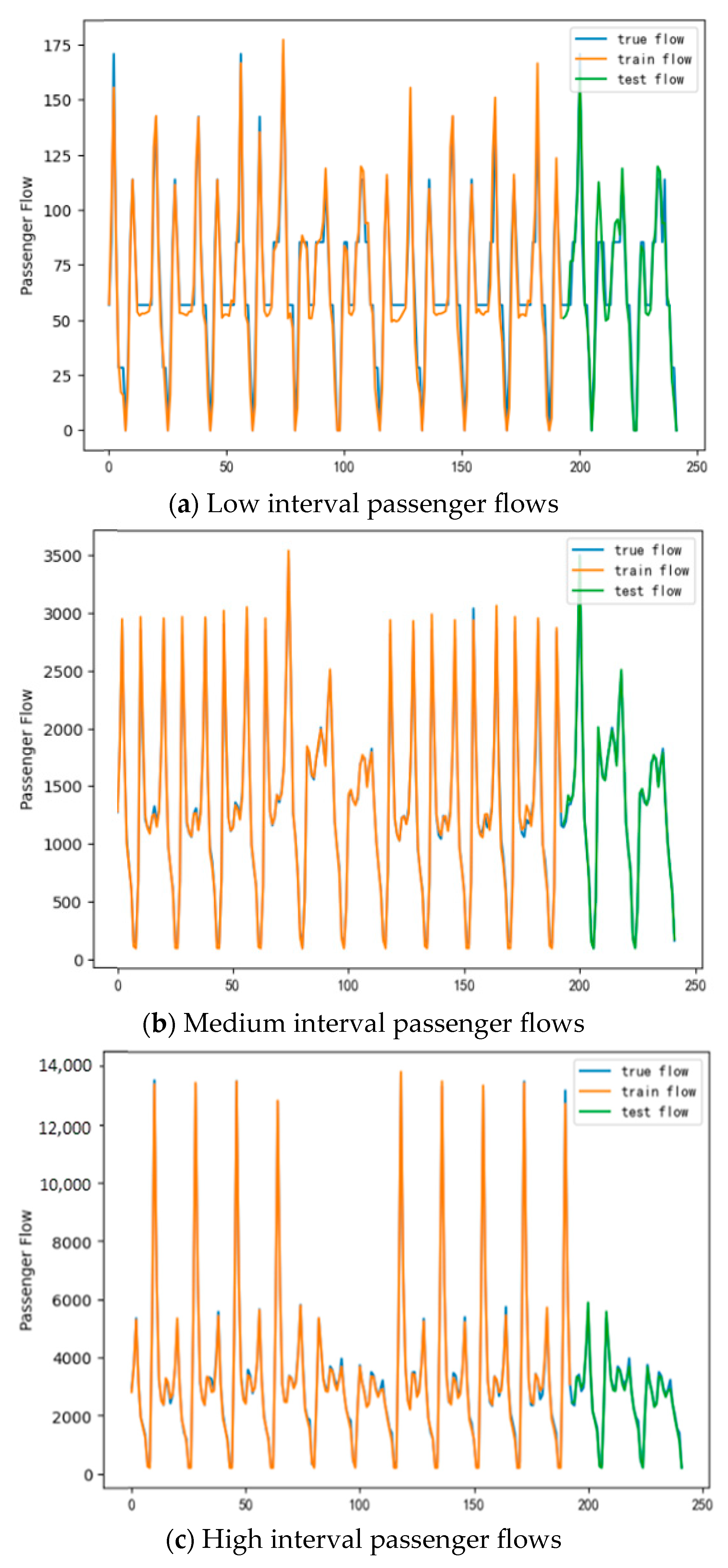
Figure 12 shows the predicted results of three typical passenger flow intervals. The horizontal coordinate is the time series index, indicating the sample number of OD passenger flow in a single day, and the ordinate is the OD passenger flow. It can be seen that the test values fit well with the true values, indicating that the deep learning model designed in this study can to some extent capture the changing characteristics of OD passenger flow and reflect the changing patterns of OD passenger flow.
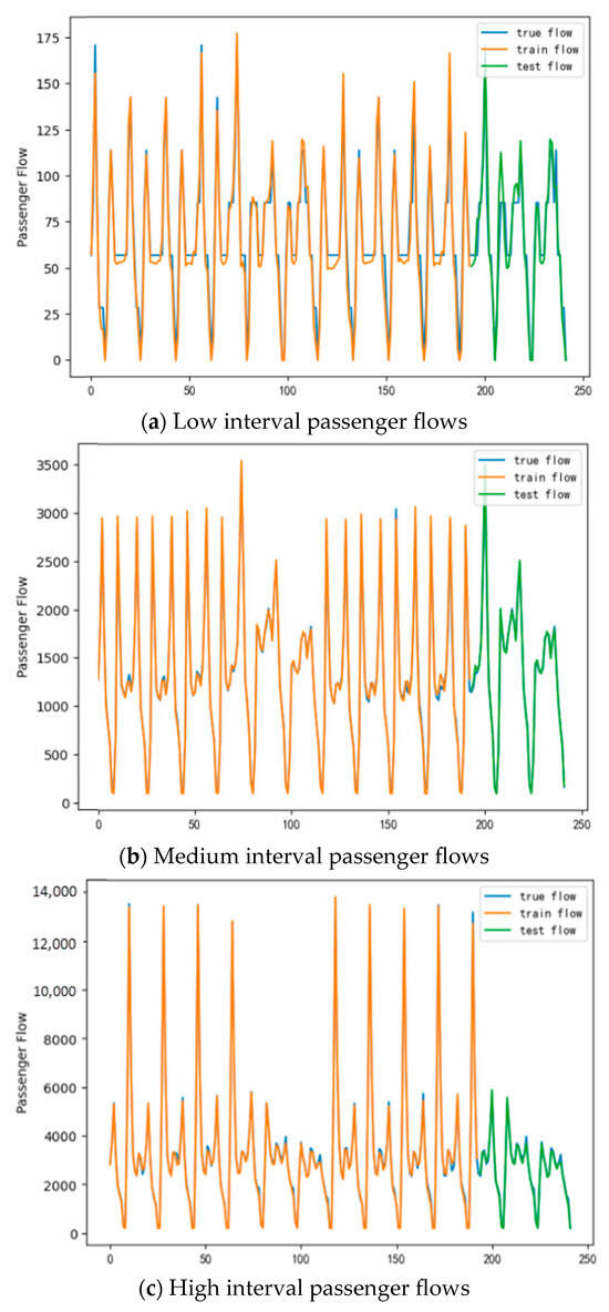
Figure 12.
Short-term OD passenger flow prediction results.
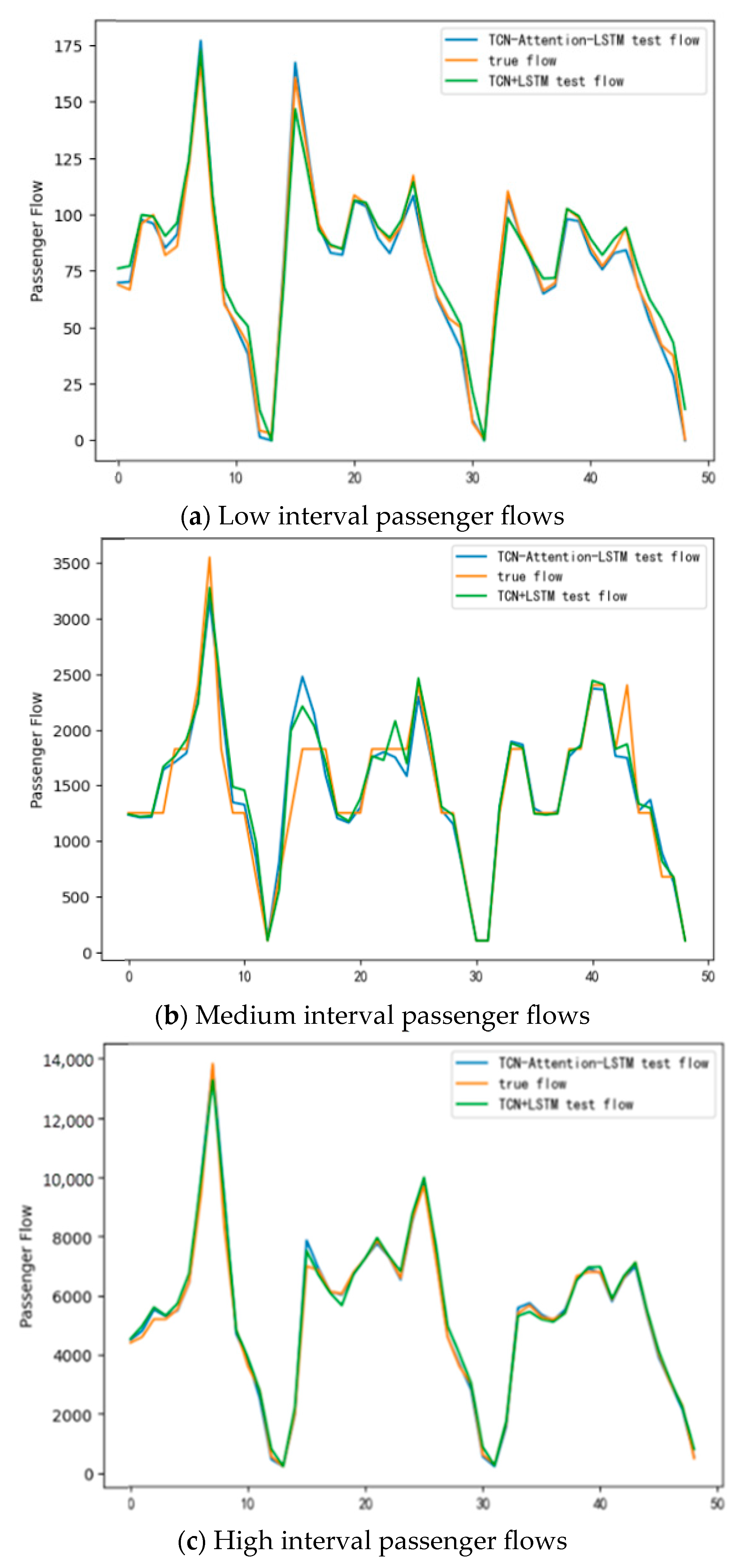
Further analysis was conducted on the prediction accuracy of the TCN–Attention–LSTM model under different levels of OD passenger flow, and the TCN-LSTM baseline model was also used to predict OD passenger flow. The introduction of the TCN-LSTM combination model can be found in our previous paper, which has been successfully applied to station passenger flow prediction [29]. Afterwards, the predicted value of the TCN-LSTM model based on the passenger flow output of the interval and the output predicted value of the TCN–Attention–LSTM model are compared with the corresponding real value in the three typical sections selected. The results are shown in Figure 13. From the prediction results in the figure, it can be seen that the data curve of the TCN–Attention–LSTM model for passenger flow prediction can fit the data curve of real passenger flow well and better predict the peak OD passenger flow in different periods. However, the TCN-LSTM model lacks an attention mechanism to extract key information, resulting in a large prediction error for the peak OD passenger flow.
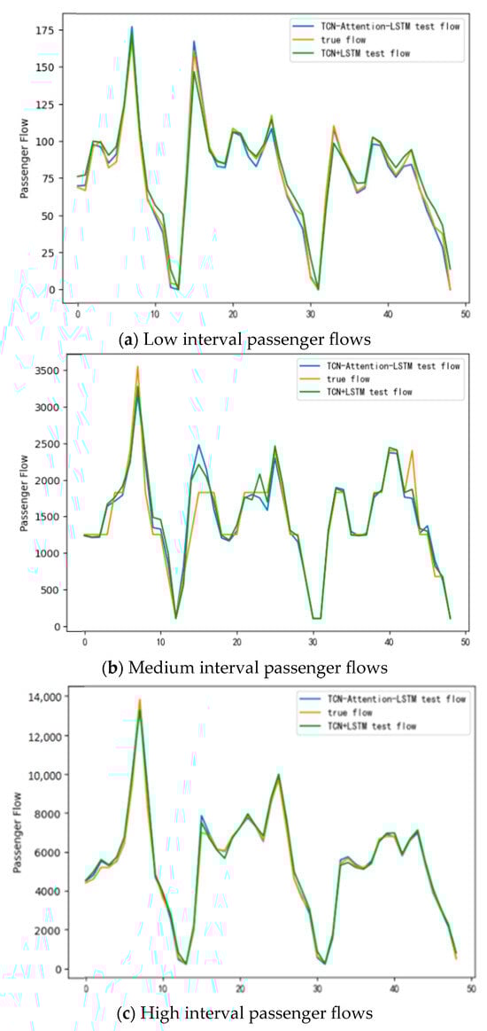
Figure 13.
Comparison results of OD passenger flow prediction.
The comparison of the prediction results of the two models shows that the TCN–Attention–LSTM model has excellent performance in predicting short-term OD passenger flow and captures the corresponding temporal and spatial characteristics. By introducing an attention mechanism, the LSTM model can adaptively adjust the attention to different time steps in the input sequence, better capture important information in the sequence, and reduce attention to irrelevant information. This can enhance the modeling ability of the model for time series and improve predictive performance.
4.3. Model Comparison and Evaluation
In order to better compare the predictive performance of the TCN–Attention–LSTM model constructed in this study, according to different intervals, the models are quantified by two common evaluation indicators, root mean square error (RMSE) and mean absolute error (MAE). The calculation formula is as follows:
where N is the total sample of the OD passenger flow prediction, xi is the actual OD passenger flow, and pi is the predicted OD passenger flow.
The mean square error is used to explain the statistical dispersion of the prediction results of passenger flow. The mean absolute error can better reflect the actual situation of the error of the prediction results of interval passenger flow.
For a comparison of the accuracy of the TCN–Attention–LSTM model with the TCN-LSTM model and a comparison of the RMSE of the prediction results of interval passenger flow of the TCN–Attention–LSTM model with the MSE and MAE of the OD passenger flow prediction results of the TCN-LSTM model, the results are shown in Table 7.
Table 7.
RMSE and MAE of TCN–Attention–LSTM model and TCN-LSTM model.
From the prediction results of the above example, compared with the TCN-LSTM model, the prediction accuracy of the TCN–Attention–LSTM model is greatly improved. From Table 6, it can be seen that compared with the TCN-LSTM model, the RMSE index of the prediction results of TCN–Attention–LSTM model decreases by 45.0%, 29.1%, and 8.7% in the high (from Jiazhoulu to Guanyinqiao), middle (Guanyinqiao to Huaxinjie), and low (Sigongli to Nanping) OD passenger flows, respectively. The MAE index decreases by 55.2%, 31.4%, and 7.0%, respectively, in the high (from Jiazhoulu to Guanyinqiao), middle (Guanyinqiao to Huaxinjie), and low (Sigongli to Nanping) OD passenger flows. The prediction results indicate that the TCN–Attention–LSTM deep learning model proposed in this study has high prediction accuracy. Even in the case of low OD passenger flow, the results are still at a high level and better than the baseline model, confirming that the OD passenger flow prediction method considering the external environmental impact of urban rail transit in this paper has high adaptability.
To further validate the efficacy of our model, we conducted a comparative analysis against the integrated models presented in references [30,31,32], which served as our baseline. While these methodologies demonstrate commendable performance in forecasting passenger flow at individual stops using singular models, combined models, and attention mechanisms, their effectiveness diminishes when applied to the prediction of short-term regional origin–destination (OD) passenger flows. Specifically, their predictive accuracy falls short of expectations, with notably higher errors compared to our proposed model. This discrepancy underscores the necessity for a more nuanced approach to OD flow prediction, as highlighted by our analysis and comparison with existing works.
By combining different OD passenger flow prediction curves, it can be found that the TCN–Attention–LSTM model has high coupling in predicting the overall trend of OD passenger flow. At the same time, the overall prediction accuracy is higher in the medium-to-high OD passenger flow range, while the prediction trend fluctuates greatly in the low-passenger-flow range, and the accuracy is unstable. The reason for this is that as the passenger flow decreases, the sample size of training data decreases, and it is less affected by external factors, resulting in an increase in the difficulty of prediction. The constructed TCN–Attention–LSTM prediction model can not only couple external weather and date factors but also better capture OD peak passenger flow than the baseline model. This leads to a significant difference in predictive performance between the two in the medium-to-high traffic range, while the OD peak in the low-passenger-flow range is lower, resulting in a smaller difference in prediction.
In addition, the results of OD passenger flow prediction also indicate that the baseline model TCN-LSTM can carry out prediction work, but further optimization is still needed. This also indicates that as the complexity of the actual situation increases, the prediction models supported by the TCN-LSTM model have a hard time meeting practical needs.
5. Conclusions
In order to achieve an accurate prediction of OD passenger flow in urban rail transit and improve the operational efficiency and service quality of urban rail transit, this study constructed a TCN–Attention–LSTM OD passenger flow prediction model. Firstly, the characteristics of OD passenger flow in urban rail transit were analyzed. Then, a deep learning model was used for passenger flow prediction, and external weather and date factors were coupled for prediction analysis. The results indicate the following:
- (1)
- A spatiotemporal distribution analysis was conducted on the OD passenger flow of Chongqing Rail Transit Line 3, and it was found that there was a bimodal pattern of morning and evening OD flow, with the passenger flow on weekdays being greater than that on rest days. The analysis of factors affecting OD passenger flow shows that date attributes, time attributes, and air quality have a significant impact on OD passenger flow data. This can provide a good dataset for accurately predicting OD passenger flow in urban rail transit in the future.
- (2)
- The TCN-LSTM model, which combines the attention mechanism, has better prediction accuracy than the original TCN-LSTM model, and the prediction results are more in line with the actual changes in OD passenger flow.
- (3)
- The attention mechanism can compensate for the shortcomings of the TCN-LSTM model in actual OD passenger flow prediction. The RMSE and MAE values of its prediction results are significantly reduced. The TCN-LSTM model mixed with the attention mechanism performs better than the TCN-LSTM model in predicting OD passenger flow and can more accurately predict OD passenger flow in rail transit.
- (4)
- The OD passenger flow prediction work of urban rail transit carried out in this study can provide some technical support for rail transit line planning and vehicle scheduling in large cities. At the same time, the proposed prediction method is not only applicable to new line expansion scenarios based on existing infrastructure, but also applicable to the future development of intelligent rail transit systems, such as urban rail transit systems based on virtual coupling technology.
Author Contributions
Conceptualization, Z.H.; data curation, J.H.; methodology, Z.H.; software, Z.H.; validation, G.Y.; visualization, J.H.; writing—original draft, Z.H.; writing—review and editing, G.Y. All authors have read and agreed to the published version of the manuscript.
Funding
This work was supported by the National Natural Science Foundation of China (Grant No. 52072054); the Science and Technology Research Program of Chongqing Municipal Education Commission (Grant No. KJQN202100729); and the Natural Science Foundation of Chongqing, China, (Grant No. cstc2021jcyjmsxmX0534). The authors are deeply grateful for this support.
Institutional Review Board Statement
Not applicable.
Informed Consent Statement
Not applicable.
Data Availability Statement
The datasets utilized and analyzed in the present study can be obtained from the corresponding author upon reasonable request. The data are not publicly available due to privacy and ethical considerations, as they contain sensitive information that could compromise the confidentiality of the participants. Access to the data will be granted in compliance with institutional and legal requirements to ensure the protection of participant identities.
Acknowledgments
The comments of the anonymous reviewers have improved the quality of this paper and are also gratefully acknowledged.
Conflicts of Interest
The authors declare no conflicts of interest.
References
- Yi, P.Y.; Huang, F.H.; Wang, J.C.; Peng, J. Topology augmented dynamic spatial-temporal network for passenger flow forecasting in urban rail transit. Appl. Intell. 2023, 53, 24655–24670. [Google Scholar] [CrossRef]
- Willumsen, L.G. Estimating Time-Dependent Trip Matrices from Traffic Counts. In Proceedings of the Ninth International Symposium on Transportation and Traffic Theory, Utrecht, The Netherlands, 11–13 July 1984; VNU Science Press: Utrecht, The Netherlands, 1984; pp. 397–411. [Google Scholar]
- Lam, W.H.K.; Lo, H.P. Estimation of Origin-Destination Matrix from Traffic Counts: A Comparison of Entropy Maximizing and Information Minimizing Models. Transp. Plan. Technol. 1991, 16, 85–104. [Google Scholar] [CrossRef]
- Wu, J. A Real-Time Origin-Destination Matrix Updating Algorithm for On-Line Applications. Transp. Res. Part B Methodol. 1997, 31, 381–396. [Google Scholar] [CrossRef]
- Cascetta, E.; Nguyen, S. A Unified Framework for Estimating or Updating Origin/Destination Matrices from Traffic Counts. Transp. Res. Part B Methodol. 1988, 22, 437–455. [Google Scholar] [CrossRef]
- Cascetta, E. Estimation of Trip Matrices from Traffic Counts and Survey Data: A Generalized Least Squares Estimator. Transp. Res. Part B Methodol. 1984, 18, 289–299. [Google Scholar] [CrossRef]
- Tebaldi, C.; West, M. Bayesian Inference on Network Traffic Using Link Count Data. J. Am. Stat. Assoc. 1998, 93, 557–573. [Google Scholar] [CrossRef]
- Bhattacharjee, D.; Sinha, K.C.; Krogmeier, J.V. Modeling the Effects of Traveler Information on Freeway Origin Destination Demand Prediction. Transp. Res. Part C Emerg. Technol. 2001, 9, 381–398. [Google Scholar] [CrossRef]
- Silva, R.; Kang, S.M.; Airoldi, E.M. Predicting Traffic Volumes and Estimating the Effects of Shocks in Massive Transportation Systems. Proc. Natl. Acad. Sci. USA 2015, 112, 5643–5648. [Google Scholar] [CrossRef]
- Leng, B.; Zeng, J.; Xiong, Z. Probability Tree Based Passenger Flow Prediction and Its Application to the Beijing Subway System. Front. Comput. Sci. China 2013, 7, 195–203. [Google Scholar] [CrossRef]
- Zou, L.M.; Wang, Z.J.; Guo, R. Real-time prediction of transit origin–destination flows during underground incidents. Transp. Res. Part C Emerg. Technol. 2024, 163, 104622. [Google Scholar] [CrossRef]
- Fu, R.; Zhang, Z.; Li, L. Using LSTM and GRU Neural Network Methods for Traffic Flow Prediction. In Proceedings of the Youth Academic Conference of Chinese Association of Automation, Wuhan, China, 11–13 November 2016; pp. 324–328. [Google Scholar]
- Ma, C.X.; Liu, T. Survey of short-term traffic flow prediction based on LSTM. Int. J. Mod. Phys. C 2025, 36, 2450177. [Google Scholar] [CrossRef]
- Zhang, J.; Li, H.; Zhang, S.; Yang, L.; Jin, G.; Qi, J. A spatiotemporal graph generative adversarial networks for short-term passenger flow prediction in urban rail transit systems. Int. J. Gen. Syst. 2023, 52, 694–721. [Google Scholar] [CrossRef]
- Ye, J.X.; Zhao, J.J.; Zheng, F.R.; Xu, C.Z. A Heterogeneous Graph Convolution Based Method for Short-Term OD Flow Completion and Prediction in a Metro System. IEEE Trans. Intell. Transp. Syst. 2024, 25, 15614–15627. [Google Scholar] [CrossRef]
- Wu, J.; He, D.; Jin, Z.; Li, X.; Li, Q.; Xiang, W. Learning spatial–temporal pairwise and high-order relationships for short-term passenger flow prediction in urban rail transit. Expert Syst. Appl. 2024, 245, 123091. [Google Scholar] [CrossRef]
- Miao, H.; Fei, Y.; Wang, S.; Wang, F.; Wen, D. Deep learning based origin-destination prediction via contextual information fusion. Multimed. Tools Appl. 2022, 81, 12029–12045. [Google Scholar] [CrossRef]
- Zou, X.; Zhang, S.; Zhang, C.; James, J.Q.; Chung, E. Long-Term Origin-Destination Demand Prediction with Graph Deep Learning. IEEE Trans. Big Data 2022, 8, 1481–1495. [Google Scholar] [CrossRef]
- Wang, L.G.; Dong, Y.F.; Wang, Y.Z.; Wang, P. Non-Symmetric Spatial-Temporal Network for Bus Origin-Destination Demand Prediction. Transp. Res. Rec. 2022, 2676, 279–289. [Google Scholar] [CrossRef]
- Lv, S.R.; Wang, K.P.; Yang, H.; Wang, P. An origin–destination passenger flow prediction system based on convolutional neural network and passenger source-based attention mechanism. Expert Syst. Appl. 2024, 238, 121989. [Google Scholar] [CrossRef]
- Zhang, W.; Wang, G.; Liu, X.; Zhu, T. AttnOD: An Attention-Based OD Prediction Model with Adaptive Graph Convolution. In International Conference on Neural Information Processing; Springer: Singapore, 2023. [Google Scholar]
- Liu, J.W.; Pan, L.; Ren, Q.Q. Spatial-temporal memory enhanced multi-level attention network for origin-destination demand prediction. Complex Intell. Syst. 2024, 10, 6435–6448. [Google Scholar] [CrossRef]
- Zeng, J.; Tang, J. Combining knowledge graph into metro passenger flow prediction: A split-attention relational graph convolutional network. Expert Syst. Appl. 2023, 213, 118790. [Google Scholar] [CrossRef]
- Kanungo, T.; Mount, D.M.; Netanyahu, N.S.; Piatko, C.D.; Silverman, R.; Wu, A.Y. An Efficient k-means Clustering Algorithm: Analysis and Implementation. IEEE Trans. Pattern Anal. Mach. Intell. 2002, 24, 881–892. [Google Scholar] [CrossRef]
- Guo, Y.; Zhu, Z.; Jiang, X.; Chen, T.; Li, Q. Analyzing the Impacts of Land Use and Network Features on Passenger Flow Distribution at Urban Rail Stations from a Classification Perspective. Sustainability 2024, 16, 3568. [Google Scholar] [CrossRef]
- Liu, P.F.; Wang, S.C.; Zhao, P. Robust estimation and test for Pearson’s correlation coefficient. Random Matrices Theory Appl. 2024, 13, 2450023. [Google Scholar] [CrossRef]
- Ejegwa, P.A.; Wanzenke, T.D.; Ogwuche, I.O.; Anum, M.T.; Isife, K.I. A robust correlation coefficient for fermatean fuzzy sets based on spearman’s correlation measure with application to clustering and selection process. J. Appl. Math. Comput. 2024, 70, 1747–1770. [Google Scholar] [CrossRef]
- Rossello, X. The P-value spectrum: From ‘absence of evidence’ to ‘evidence of difference’. Eur. Heart J. Acute Cardiovasc. Care 2024, 13, 181–182. [Google Scholar] [CrossRef] [PubMed]
- Hou, Z.; Du, Z.; Yang, G.; Yang, Z. Short-term passenger flow prediction of urban rail transit based on a combined deep learning model. Appl. Sci. 2022, 12, 7597. [Google Scholar] [CrossRef]
- Wei, L.; Guo, D.; Chen, Z.; Yang, J.; Feng, T. Forecasting Short-Term Passenger Flow of Subway Stations Based on the Temporal Pattern Attention Mechanism and the Long Short-Term Memory Network. ISPRS Int. J. Geo-Inf. 2023, 12, 25. [Google Scholar] [CrossRef]
- Zhao, Q.L.; Feng, X.B.; Zhang, L.W.; Wang, Y.D. Research on Short-Term Passenger Flow Prediction of LSTM Rail Transit Based on Wavelet Denoising. Mathematics 2023, 11, 4204. [Google Scholar] [CrossRef]
- Ma, C.X.; Zhang, B.W.; Li, S.K.; Lu, Y.P. Urban rail transit passenger flow prediction with ResCNN-GRU based on self-attention mechanism. Phys. A Stat. Mech. Its Appl. 2024, 638, 129619. [Google Scholar] [CrossRef]


Disclaimer/Publisher’s Note: The statements, opinions and data contained in all publications are solely those of the individual author(s) and contributor(s) and not of MDPI and/or the editor(s). MDPI and/or the editor(s) disclaim responsibility for any injury to people or property resulting from any ideas, methods, instructions or products referred to in the content. |
© 2025 by the authors. Licensee MDPI, Basel, Switzerland. This article is an open access article distributed under the terms and conditions of the Creative Commons Attribution (CC BY) license (https://creativecommons.org/licenses/by/4.0/).