
Design, Modeling, and Optimization of a Nearly Constant Displacement Reducer with Completely Distributed Compliance


Abstract
:1. Introduction
- An over-constrained distributed compliant reducer is proposed, which provides a nearly constant reduction ratio across a wide range of input displacement. Simultaneously, this mechanism significantly reduces the moving lumped mass;
- The mathematical model of the displacement reducer is established based on the compliance matrix method, to predict the input–output relationship and to perform a detailed analysis of the structural sensitivity;
- A general optimization method for distributed compliance mechanisms based on the PSO algorithm is proposed. This optimization approach is applicable to the sizing optimization of most distributed compliant mechanisms. The optimization objectives under three different scenarios were considered separately.
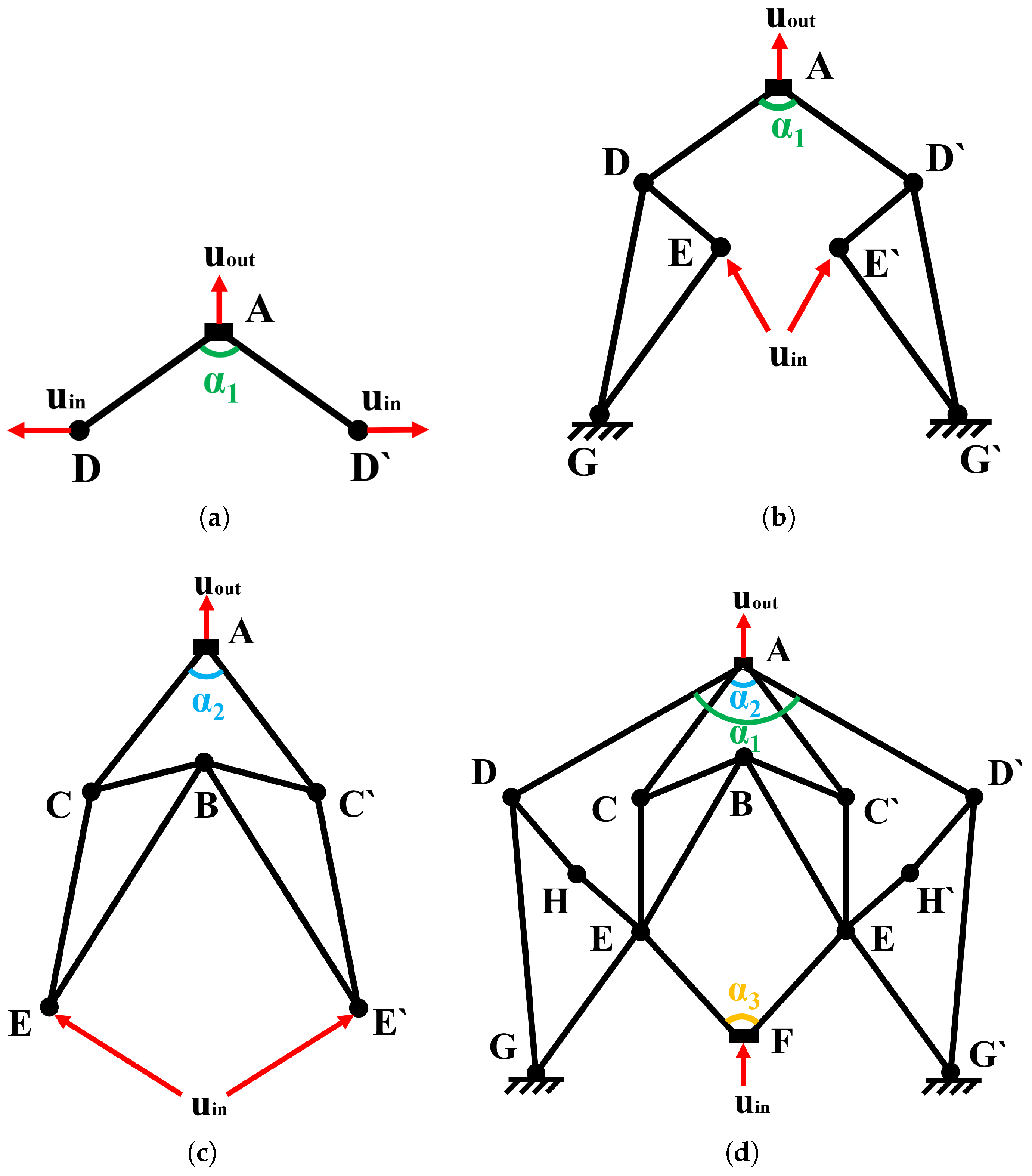
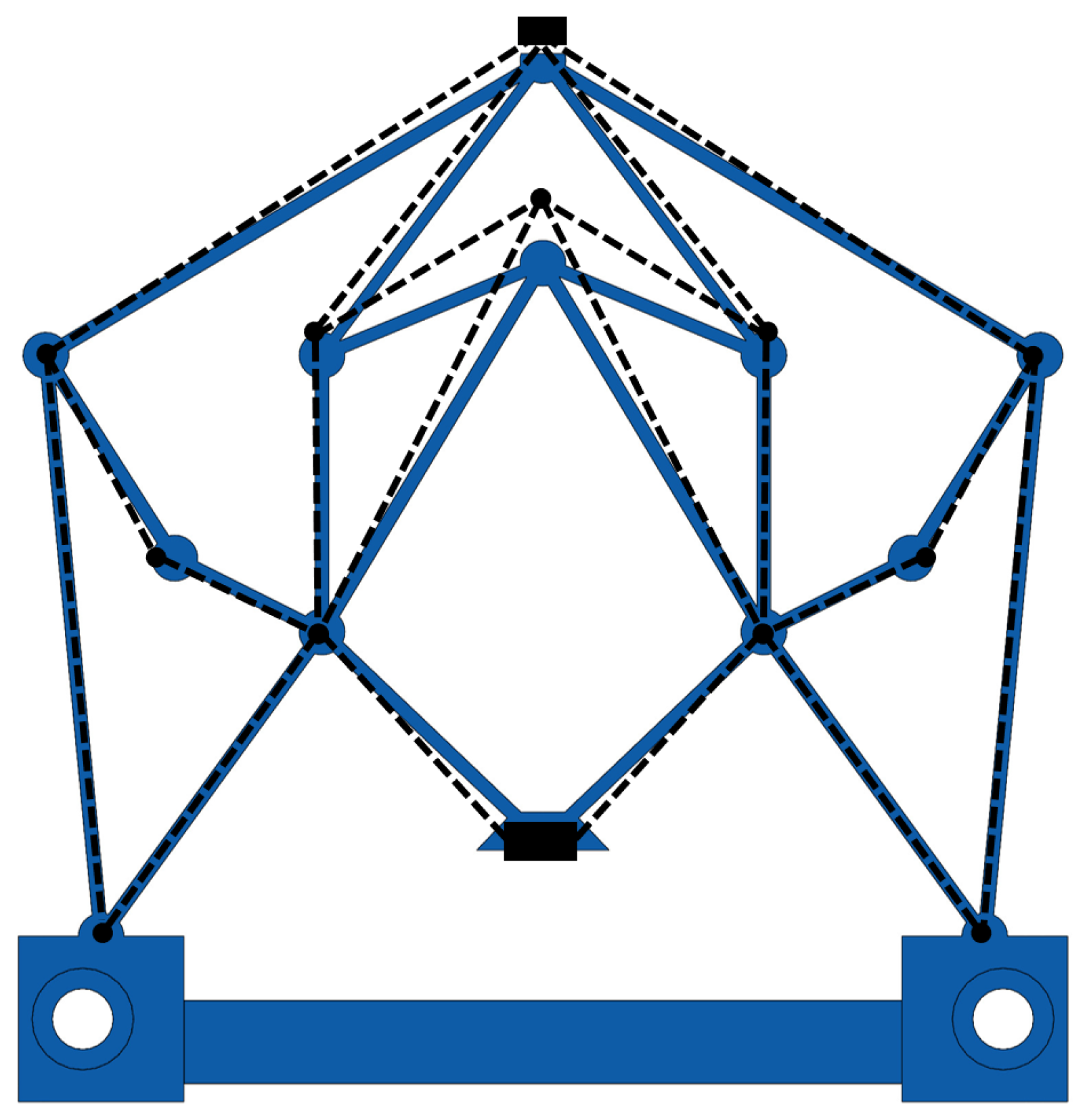
2. Mechanism Design
3. Kinetostatic Modeling and FEA
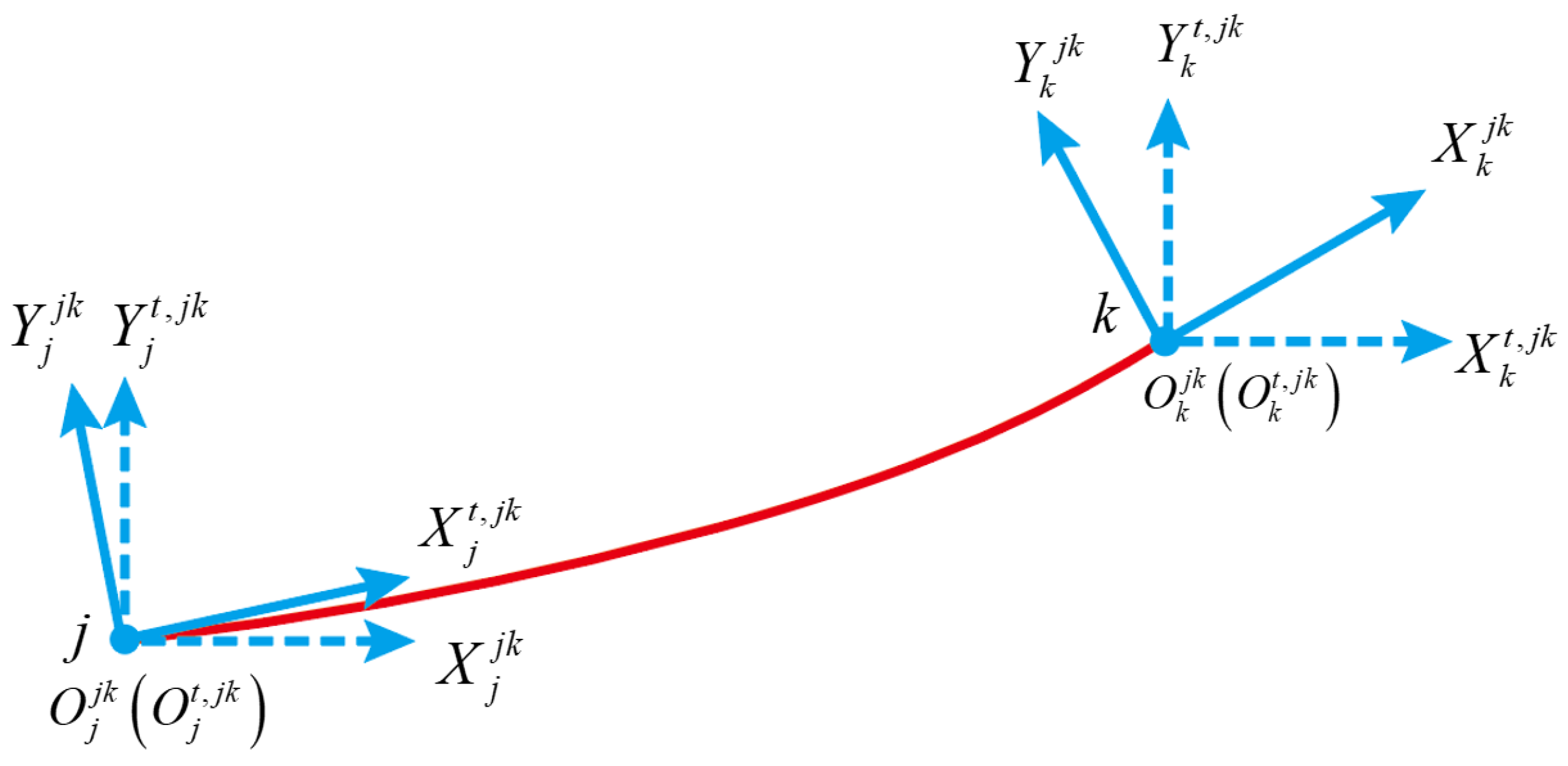
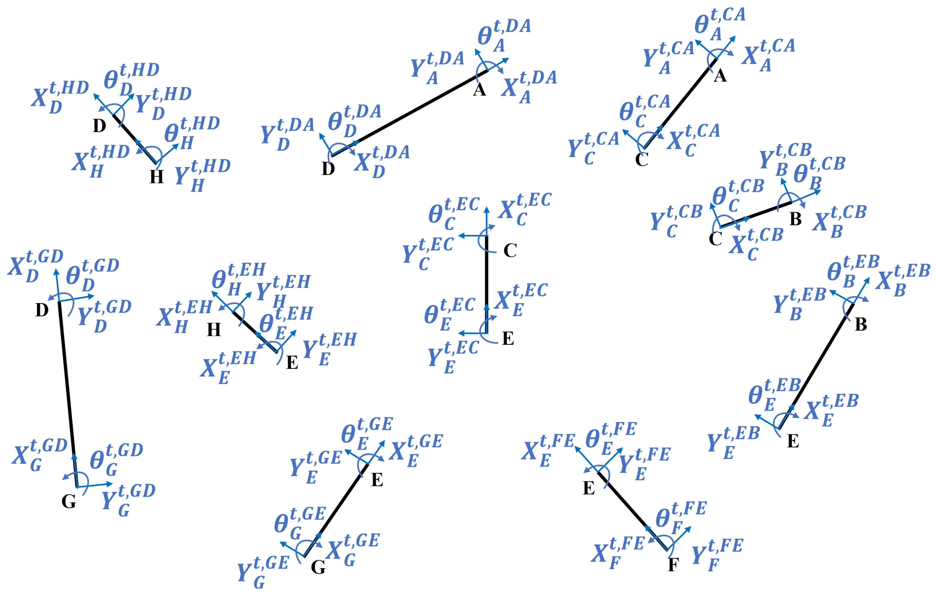
3.1. Model of Distributed Compliant Beams
3.2. Modeling of the Compliant Reducer
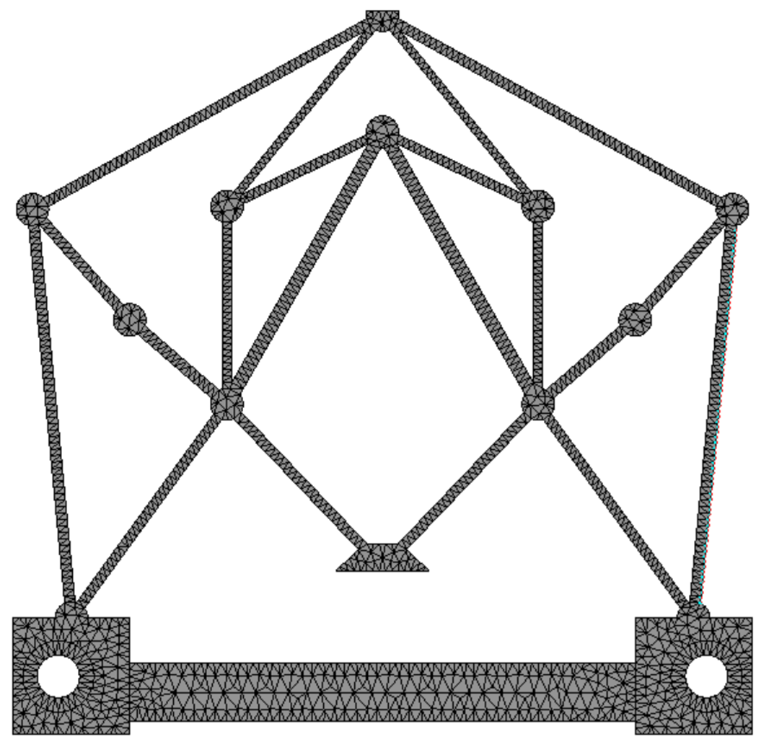
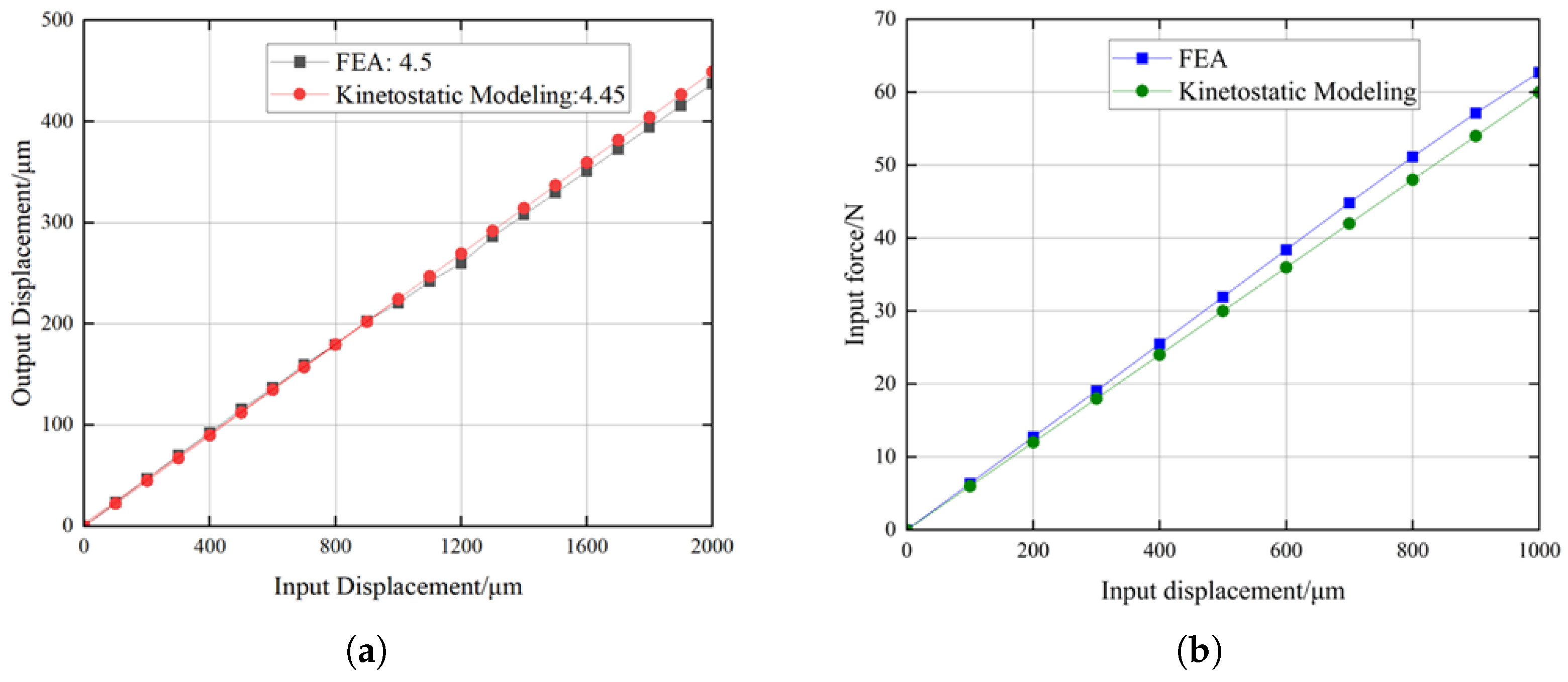
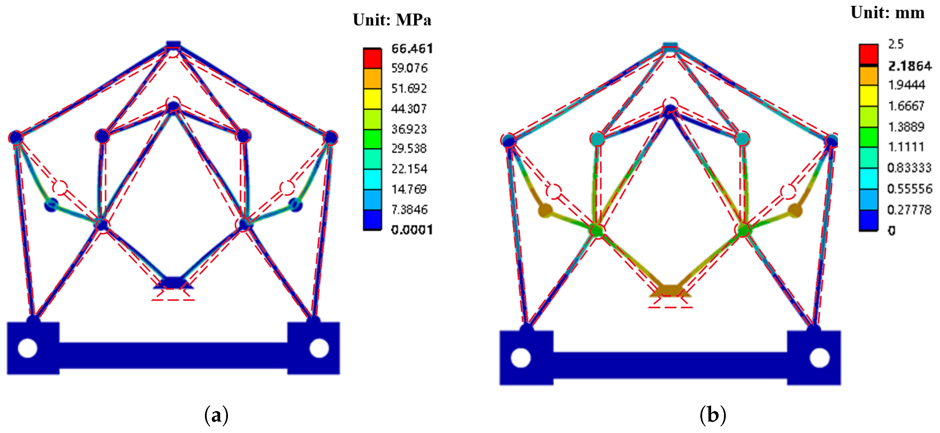
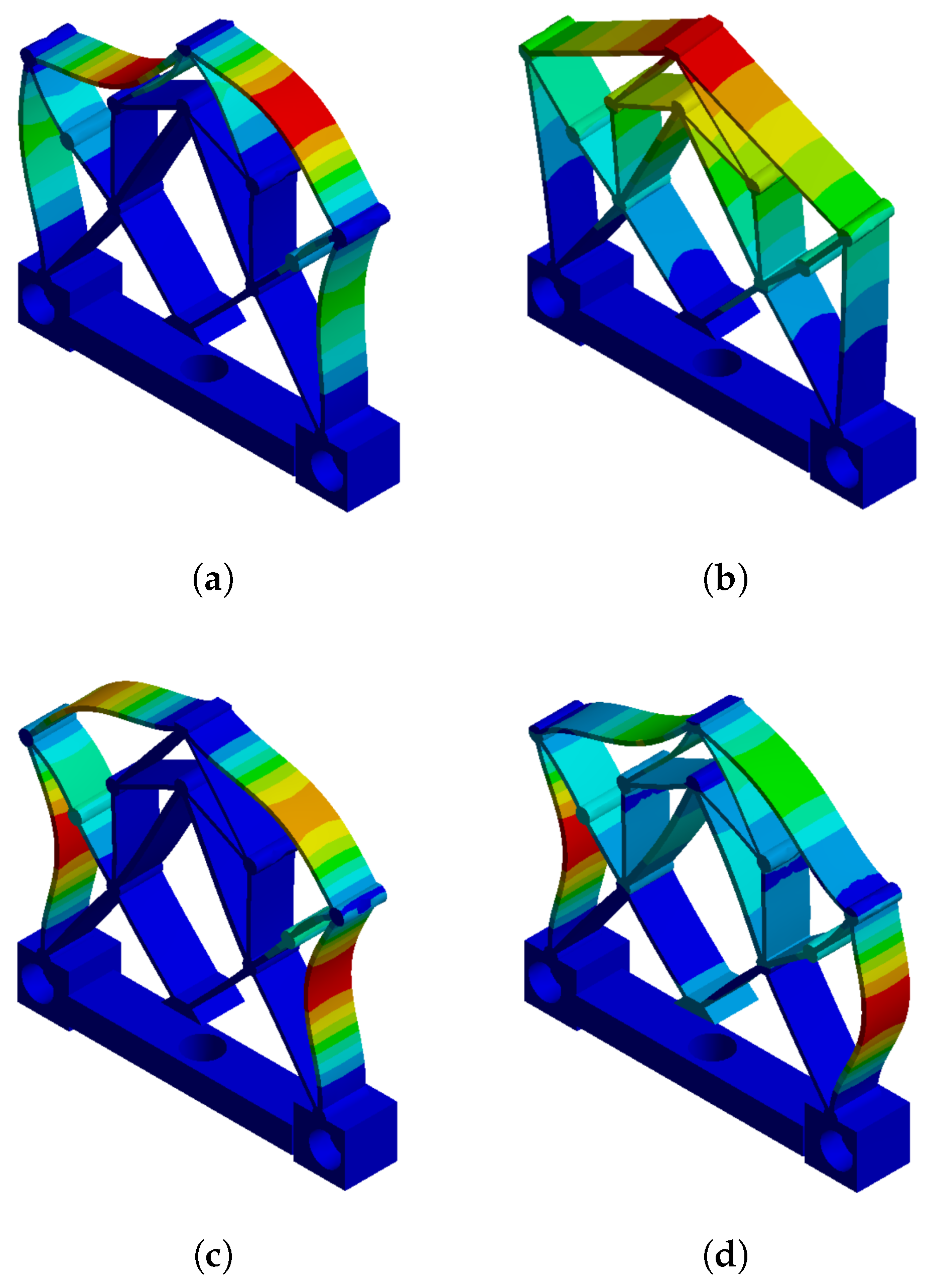
3.3. FEA Verification
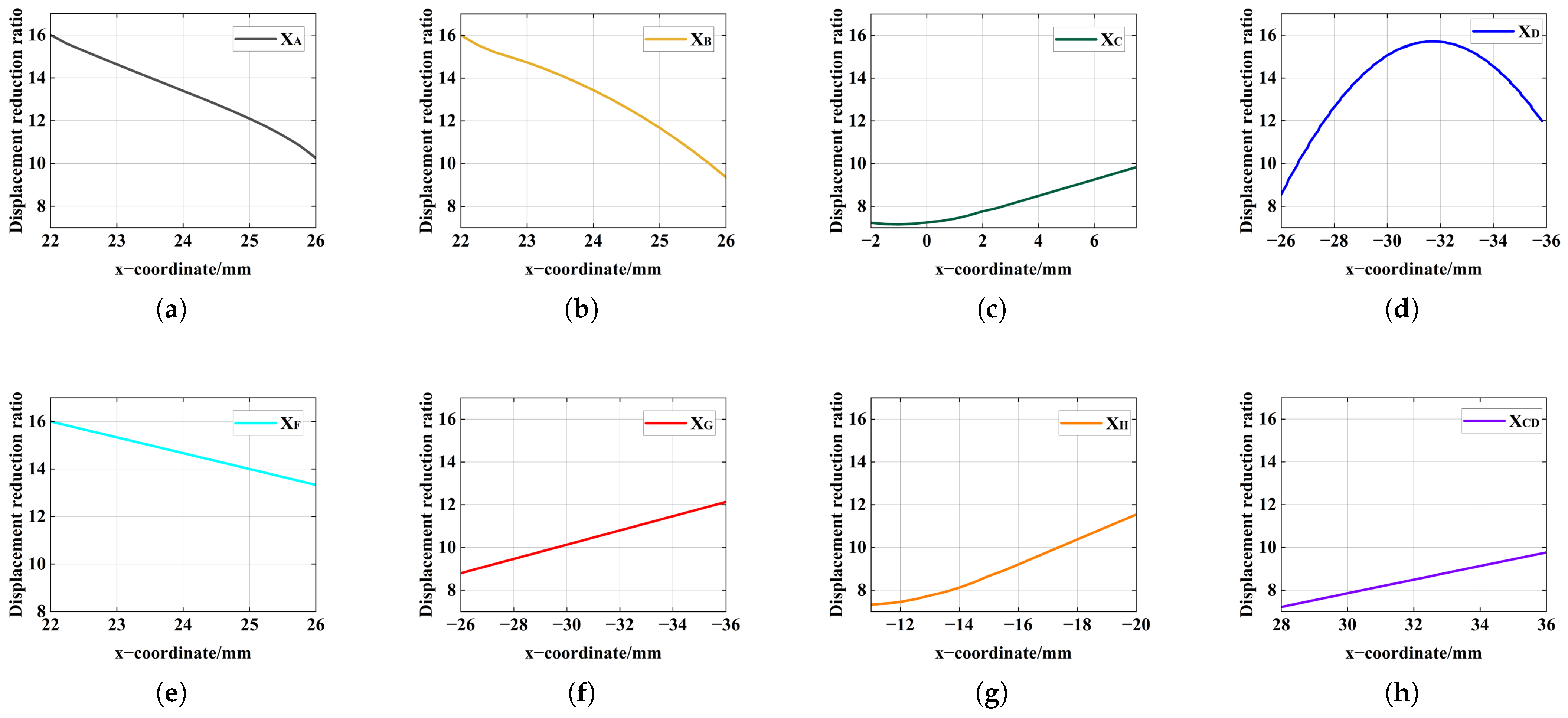
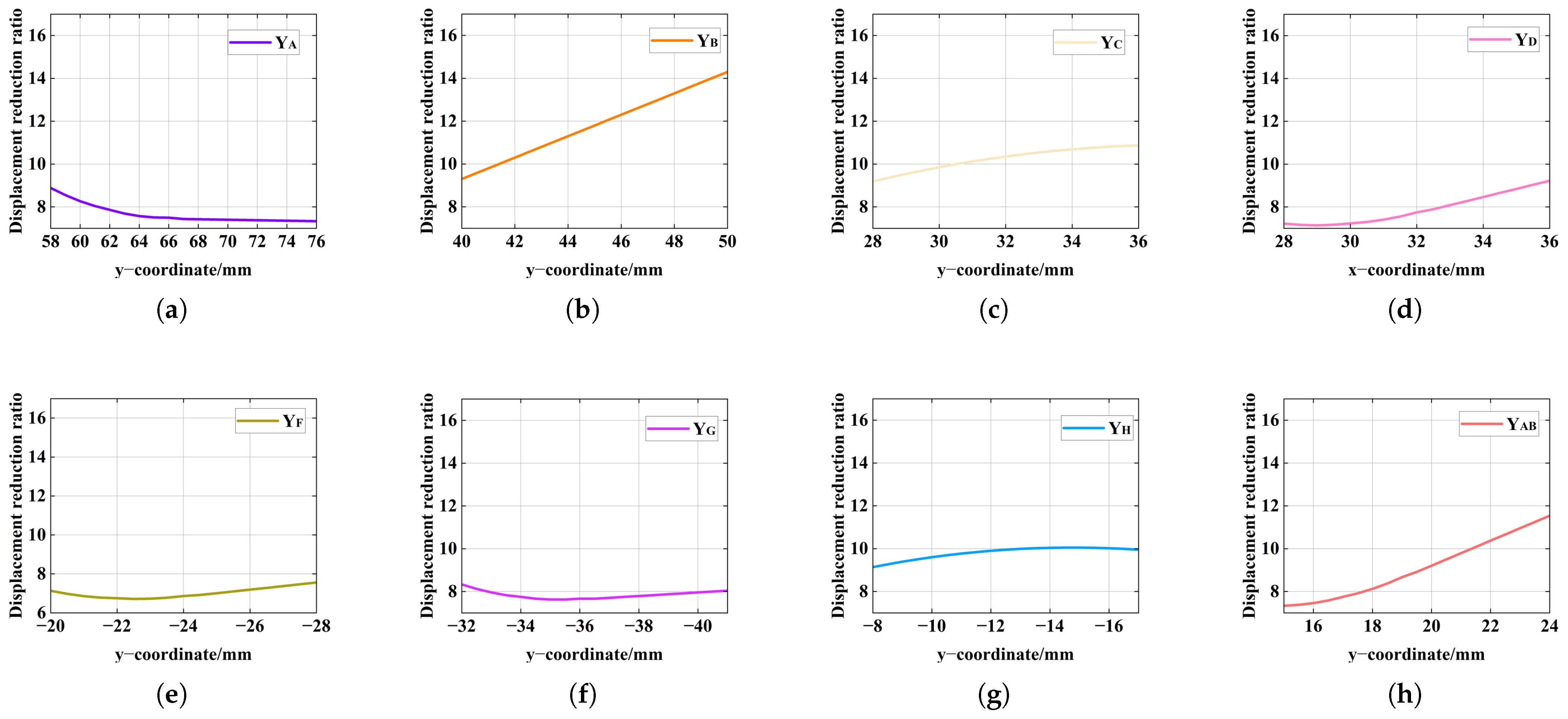
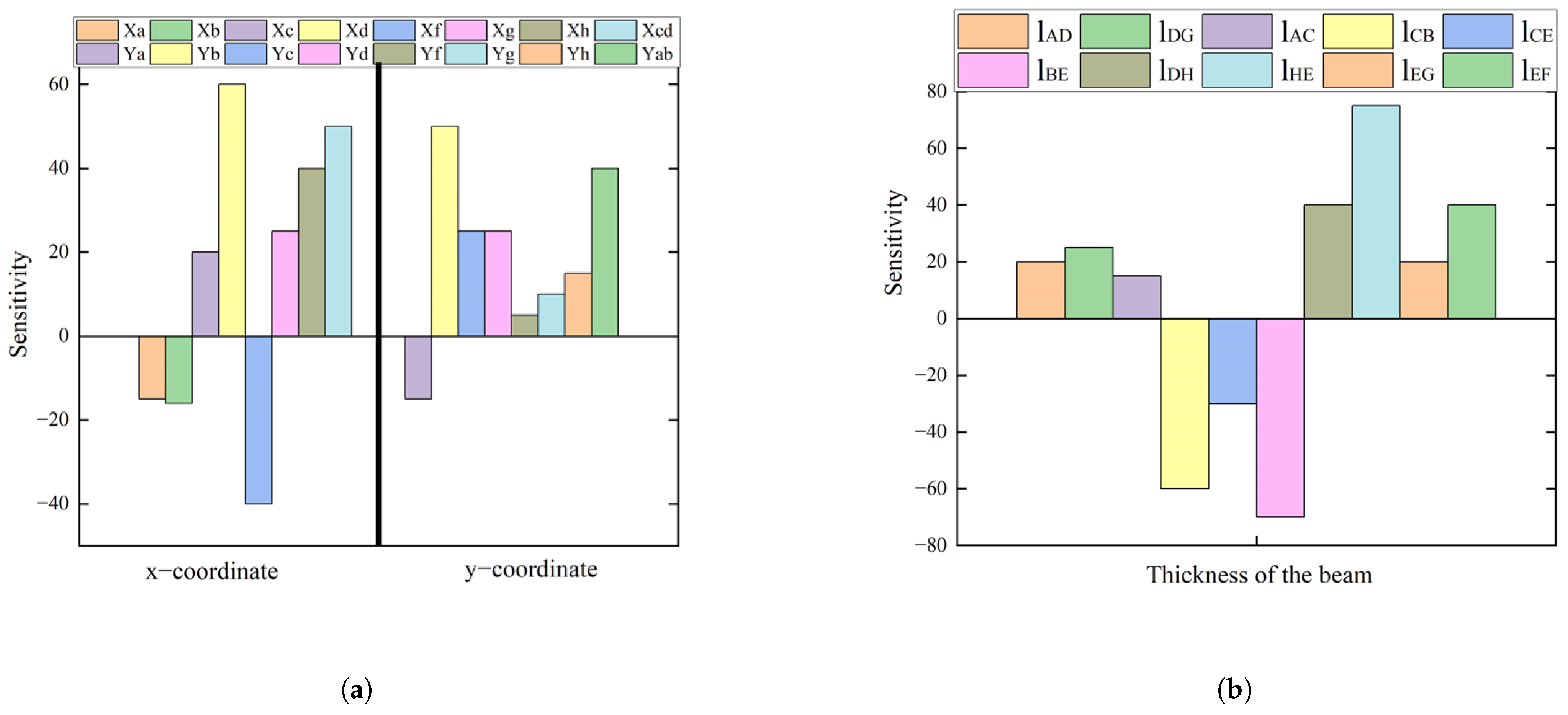
3.4. Sensitivity Analysis: Geometric Positions and Beam Width
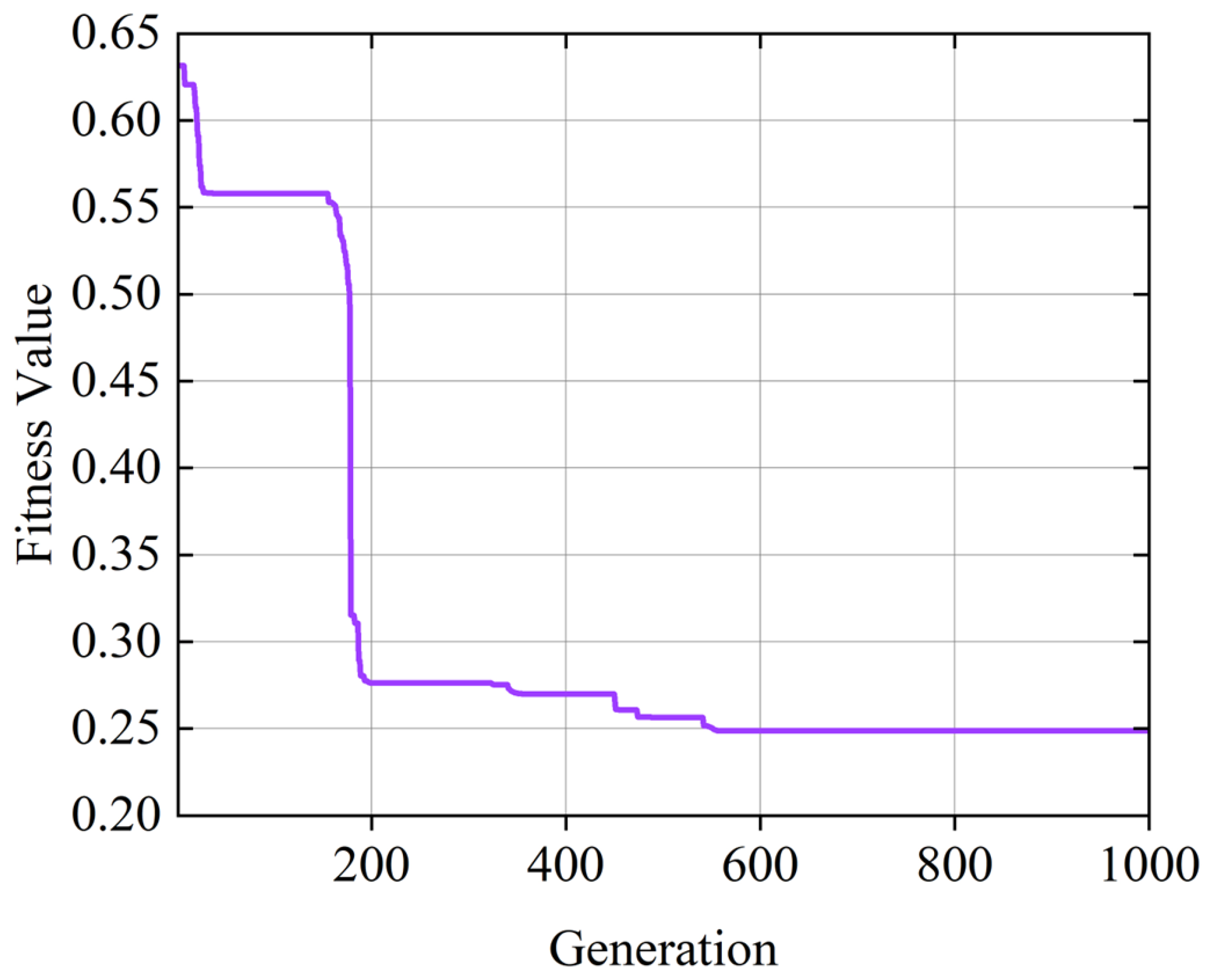
4. Structural Optimization
- Position vector : Represents the current position of the particle in the solution space, i.e., the current candidate solution;
- Velocity vector : Represents the search direction and step size of the particle in the solution space that determine the direction and speed of the particle’s next move.
- Individual best solution : The best solution found by each particle during the search process, denoted as ;
- Global best solution : The best solution found by the entire particle swarm during the search process, denoted as ;
- Inertia weight w: Used to balance global exploration and local exploitation. A larger inertia weight favors global exploration, while a smaller inertia weight helps local exploitation.
- Determine the structural parameter requirements and functional parameter indicators of the distributed compliant mechanism based on functional requirements;
- Choose an appropriate modeling method based on the functional parameter indicators and geometric parameter requirements for modeling;
- Perform a comparative optimization of structures under different optimization objectives;
- Based on the optimization results from step 3, perform weighting or constraint processing to ensure that other optimization objectives remain within a reasonable range and determine the optimal objective function.
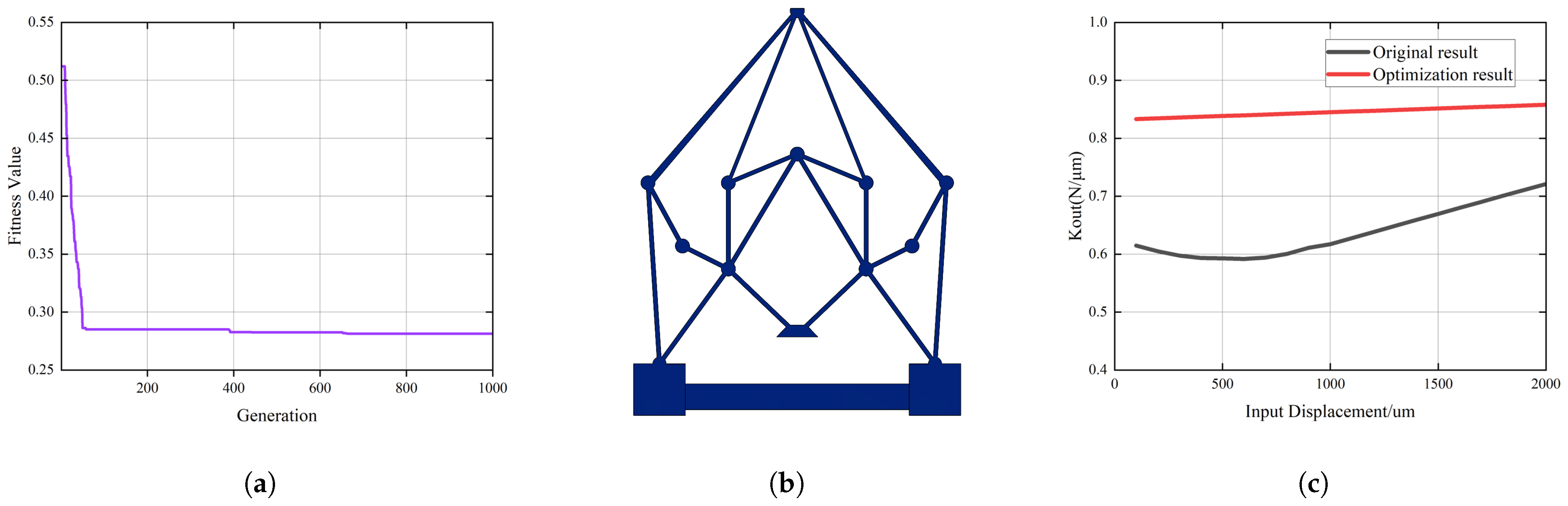
4.1. Optimization of Constant Output Stiffness
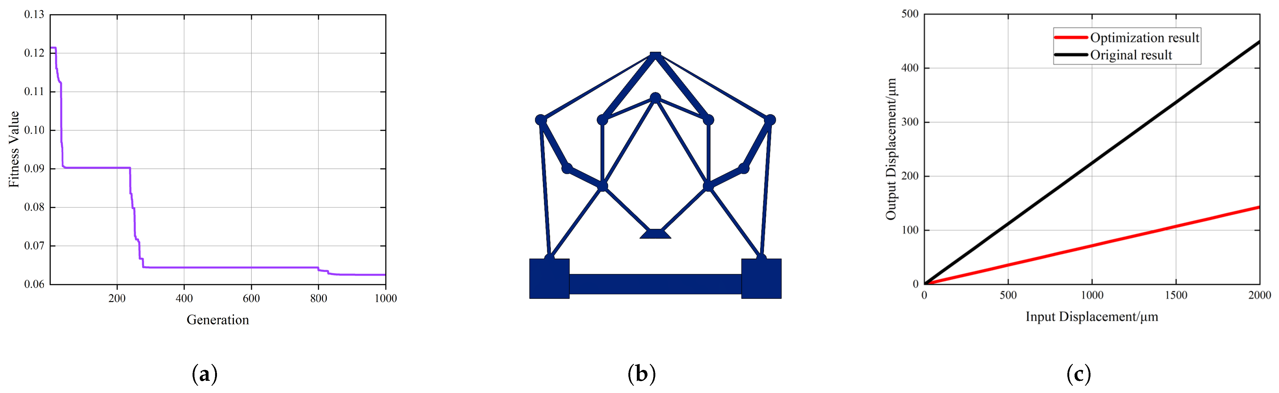
4.2. Optimization of Reduction Ratio
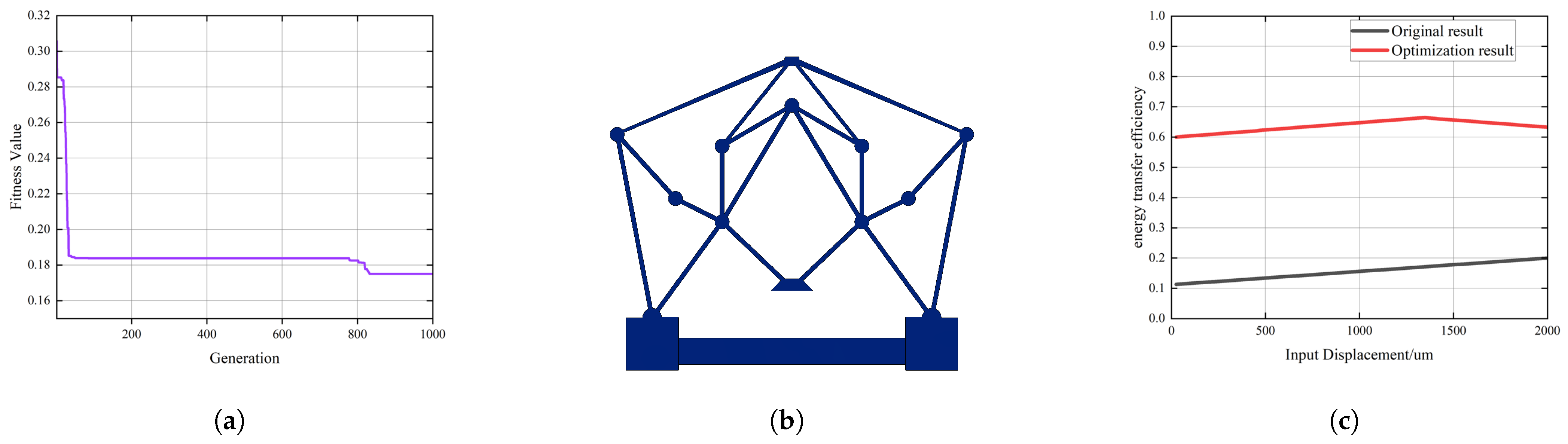
4.3. Optimization of Energy Transfer Efficiency
4.4. Comprehensive Discussion of Optimization Model
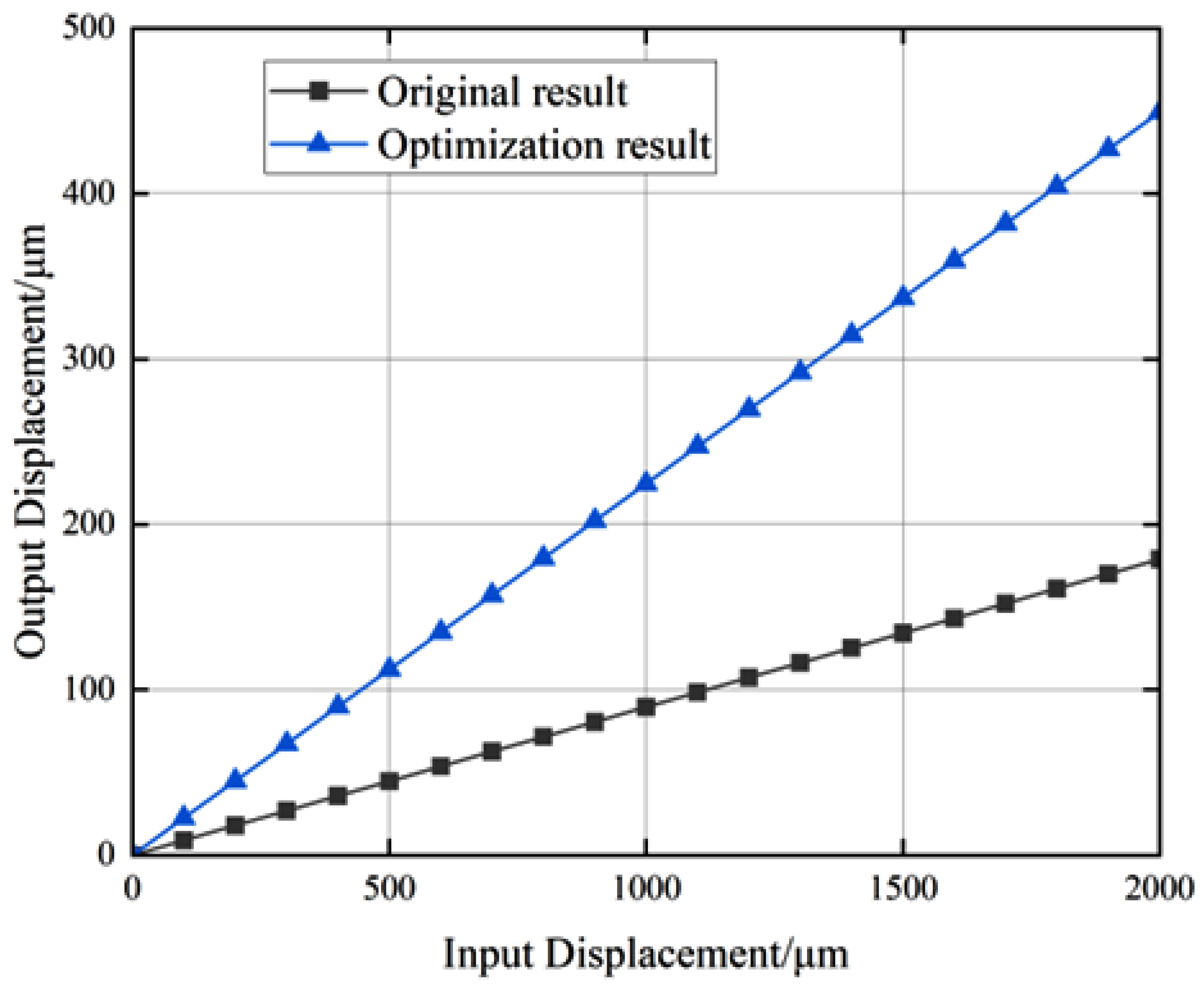
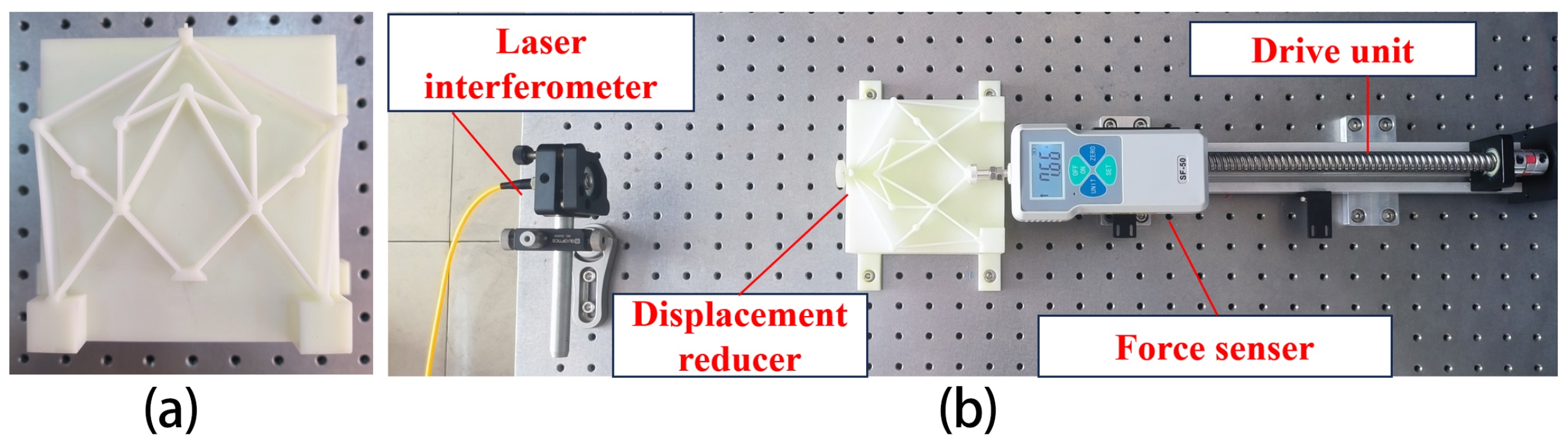
5. Experimentation
6. Conclusions
- Grounded in the principles of over-constrained design, it presents a distributed compliant reducer capable of maintaining a nearly constant reduction ratio over a wide range of input displacements, simultaneously minimizing the moving lumped mass;
- The analytical model of the mechanism is developed using the compliance matrix method, which is employed to conduct a detailed structural sensitivity analysis;
- An integrated optimization approach combining the PSO algorithm with the analytical model is applied to achieve a comprehensive optimization of the structure. This methodology is applicable for the structure optimization of most distributed compliant mechanisms;
- In the field of precision operations, such as micro-grippers, biological manipulation, and micro-alignment mechanisms, closed-loop systems with stringent environmental requirements and complex structures are commonly used to achieve high-precision positioning and operation. In contrast, the mechanism proposed in this study features a simple structure and easy fabrication, capable of achieving stable, high-precision output displacements under complex operating conditions, thus providing a more straightforward and reliable solution for precision operations.
Author Contributions
Funding
Institutional Review Board Statement
Informed Consent Statement
Data Availability Statement
Conflicts of Interest
References
- Yang, S.; Chen, W.H. A decoupled flexure-based alignment mechanism for micromanipulation. In Proceedings of the 2016 IEEE 11th Conference on Industrial Electronics and Applications (ICIEA), Hefei, China, 5–7 June 2016; pp. 1676–1681. [Google Scholar]
- Zhang, L.; Liu, P.; Yan, P. A novel compact tilt stage with additive manufacturable spatial flexure mechanism driven by asymmetric stiffness. Mech. Mach. Theory 2021, 166, 104443. [Google Scholar] [CrossRef]
- Zhao, Y.; Hao, G.; Chai, L.; Tian, Y.; Xi, F. A compliant-mechanism-based lockable prismatic joint for high-load morphing structures. Mech. Mach. Theory 2022, 178, 105083. [Google Scholar] [CrossRef]
- McGowan, P.; Hao, G. Design of a Morphing Compliant Mechanism With Separate Gripping and Retraction Modes Using a Single Actuation. J. Mech. Robot. 2023, 15, 4054551. [Google Scholar] [CrossRef]
- Liu, P.; Qian, J.; Yan, P.; Liu, Y. Design, analysis and evaluation of a self-lockable constant-force compliant gripper. Sens. Actuators Phys. 2022, 335, 113354. [Google Scholar] [CrossRef]
- Lv, B.; Lin, B.; Cao, Z.; Li, B.; Wang, G. A parallel 3-DOF micro-nano motion stage for vibration-assisted milling. Mech. Mach. Theory 2022, 173, 104854. [Google Scholar] [CrossRef]
- Toone, N.C.; Fazio, W.C. Investigation of unique carbon nanotube cell restraint compliant mechanisms. Mech. Based Des. Struct. Mach. 2014, 42, 343–354. [Google Scholar] [CrossRef]
- Van der Lee, N.; Kappelhof, P. Flexure-based alignment mechanisms: Design, development and application. In Optomechanics; SPIE: Bellingham, WA, USA, 2003; pp. 266–275. [Google Scholar]
- Lyu, Z.; Xu, Q. Design and testing of a large-workspace XY compliant manipulator based on triple-stage parallelogram flexure. Mech. Mach. Theory 2023, 184, 105287. [Google Scholar] [CrossRef]
- Abedi, K.; Shakhesi, E.; Seraj, H.; Mahnama, M.; Shirazi, F.A. Design and analysis of a 2-DOF compliant serial micropositioner based on “S-shaped” flexure hinge. Precis. Eng. 2023, 83, 228–236. [Google Scholar] [CrossRef]
- Sharafkhani, N.; Long, J.M.; Adams, S.D.; Kouzani, A.Z. A binary stiffness compliant neural microprobe. Sens. Actuators Phys. 2023, 363, 228–236. [Google Scholar] [CrossRef]
- Lyu, Z.; Xu, Q. Novel design of a piezoelectrically actuated compliant microgripper with high area-usage efficiency. Precis. Eng. 2022, 76, 1–11. [Google Scholar] [CrossRef]
- Wei, Y.; Xu, Q. Design of a new passive end-effector based on constant-force mechanism for robotic polishing. Robot. Comput.-Integr. Manuf. 2022, 74, 102278. [Google Scholar] [CrossRef]
- Guo, F.; Sun, Z.; Zhang, S.; Cao, R.; Li, H. Dynamic Characteristics and Frequency Reliability Analysis of an Optimized Compliant Stroke Amplification Mechanism. J. Mech. Robot. 2023, 15, 061007. [Google Scholar] [CrossRef]
- Iqbal, S.; Malik, A. A review on MEMS based micro displacement amplification mechanisms. Sens. Actuators Phys. 2019, 300, 111666. [Google Scholar] [CrossRef]
- Lian, J.; An, D.; Chen, M.; Huang, W.; Liang, Z. Design and feedforward control of a two-degree-of-freedom positioning stage with bidirectional piezoelectric drive. Precis. Eng. 2023, 81, 158–166. [Google Scholar] [CrossRef]
- Li, G.; Yu, J.; Pan, J.; Pei, X. Design of a Novel Flexible Spherical Hinge and Its Application in Continuum Robot. J. Mech. Robot. 2024, 16, 061012. [Google Scholar] [CrossRef]
- Chen, Y.; Lai, L. Design, Modeling, Testing, and Control of a Novel Fully Flexure-Based Displacement Reduction Mechanism Driven by Voice Coil Motor. Actuators 2022, 11, 228. [Google Scholar] [CrossRef]
- Wu, H.; Chen, G. A flexure-based displacement reducer capable of achieving very large reduction ratio. Mech. Mach. Theory 2022, 170, 104658. [Google Scholar] [CrossRef]
- Yang, M.; Sun, M.; Wu, Z.; Li, J.; Long, Y. Design of a redundant actuated 4-PPR planar 3-DOF compliant nanopositioning stage. Precis. Eng. 2023, 82, 68–79. [Google Scholar] [CrossRef]
- Jin, M.; Ynchausti, C.; Howell, L.L. Zero-curvature deformation properties and 3R pseudo-rigid-body model of large-deflection Euler spiral beams. Mech. Mach. Theory 2023, 183, 105261. [Google Scholar] [CrossRef]
- Phan, T.-V.; Truong, V.M.; Pham, H.-T.; Nguyen, V.-K. Design of a Novel Large-Stroke Compliant Constant-Torque Mechanism Based on Chained Beam-Constraint Model. J. Mech. Robot. 2024, 16, 081006. [Google Scholar] [CrossRef]
- Chen, X.; Li, Y.; Xie, Y.; Wang, R. Design and analysis of new ultra compact decoupled XYZθ stage to achieve large-scale high precision motion. Mech. Mach. Theory 2022, 167, 104527. [Google Scholar] [CrossRef]
- Xu, H.; Zhang, X.; Wang, R.; Zhang, H.; Liang, J. Design of an SMA-driven compliant constant-force gripper based on a modified chained pseudo-rigid-body model. Mech. Mach. Theory 2023, 187, 105371. [Google Scholar] [CrossRef]
- Chen, G.; Ma, Y.; Li, J. A tensural displacement amplifier employing elliptic-arc flexure hinges. Sens. Actuators Phys. 2016, 247, 307–315. [Google Scholar] [CrossRef]
- Sakuma, S.; Arai, F. Cellular force measurement using a nanometric-probe-integrated microfluidic chip with a displacement reduction mechanism. Robot. Mechatron. 2013, 25, 277–284. [Google Scholar] [CrossRef]
- Ling, M. A general two-port dynamic stiffness model and static/dynamic comparison for three bridge-type flexure displacement amplifiers. Mech. Syst. Signal Process. 2019, 119, 486–500. [Google Scholar] [CrossRef]
- Li, H.; Guo, F.; Wang, Y.; Wang, Z.; Li, C.; Ling, M.; Hao, G. Design and modeling of a compact compliant stroke amplification mechanism with completely distributed compliance for ground-mounted actuators. Mech. Mach. Theory 2022, 167, 104566. [Google Scholar] [CrossRef]
- Jiaxiang, Z.; Hao, G. Design of an over-constraint based nearly-constant amplification ratio compliant mechanism. Mech. Mach. Theory 2023, 186, 105347. [Google Scholar]
- Chen, G.; Zhang, H.; Bai, R.; Li, B. Exact constraint design of bridge-type displacement flexure amplifier. Mech. Mach. Theory 2024, 203, 105799. [Google Scholar] [CrossRef]
- Ling, M.; Zhang, X.; Cao, J. Extended Dynamic Stiffness Model for Analyzing Flexure-Hinge Mechanisms with Lumped Compliance. J. Mech. Des. 2022, 144, 4051891. [Google Scholar] [CrossRef]
- Dong, W.; Chen, F.X. Development of a highly efficient bridge-type mechanism based on negative stiffness. Smart Mater. Struct. 2017, 26, 095053. [Google Scholar] [CrossRef]


| Beam | Length | Orientation Angle | Cross-Sectional Area |
|---|---|---|---|
| Parameters | Before Optimization (mm) | Lower and Upper Limits of Width (mm) |
|---|---|---|
| 1.5 | [1,2] | |
| 1.5 | [1,2] | |
| 1.5 | [1,2] | |
| 1.5 | [1,2] | |
| 1.5 | [1,2] | |
| 1.5 | [1,2] | |
| 1.5 | [1,2] | |
| 1.5 | [1,2] | |
| 1.5 | [1,2] | |
| 1.5 | [1,2] |
| x−Coordinates | y−Coordinates | Lower and Upper | Lower and Upper | |
|---|---|---|---|---|
| Node | Before Optimization | Before Optimization | Limits of the x−Coordinates | Limits of the y−Coordinates |
| A | 24 | 60 | [20,30] | [60,70] |
| B | 24 | 44 | [20,30] | [40,50] |
| C | 0 | 32 | [0,10] | [30,40] |
| D | −30 | 30 | [−30,−20] | [20,30] |
| E | 0 | 0 | 0 | 0 |
| F | 24 | −21 | [20,30] | [−20,−10] |
| G | −24 | −33 | [−30,−20] | [−40,−30] |
| H | −15 | −8 | [−20,−10] | [−10,0] |
| Modes | 1 | 2 | 3 | 4 |
|---|---|---|---|---|
| FEA results (Hz) | 256.89 | 504.66 | 605.4 | 695.36 |
| Structure | Reduction Ratio | Structural Type | Constant Reduction Ratio Range (µm) | Moving Lumped Mass | Energy Transfer Efficiency | |
|---|---|---|---|---|---|---|
| This paper |  | 11.03 | Distributed compliance | 2000 | One input stage One output stage | 39.6% |
| Ref. [19] | 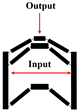 | 100 | Lumped compliance | 500 | Two input stage One output stage Other rigid bodies | 3.6% |
| Ref. [18] |  | 7.19 | Distributed compliance | 1400 | One input stage One output stage Other rigid bodies | 10% |
| Ref. [26] |  | 7.69 | Distributed compliance | 300 | One input stage One output stage | - |
| Ref. [1] |  | 8 | Lumped compliance | 200 | One input stage One output stage Other rigid bodies | - |
Disclaimer/Publisher’s Note: The statements, opinions and data contained in all publications are solely those of the individual author(s) and contributor(s) and not of MDPI and/or the editor(s). MDPI and/or the editor(s) disclaim responsibility for any injury to people or property resulting from any ideas, methods, instructions or products referred to in the content. |
© 2025 by the authors. Licensee MDPI, Basel, Switzerland. This article is an open access article distributed under the terms and conditions of the Creative Commons Attribution (CC BY) license (https://creativecommons.org/licenses/by/4.0/).
Share and Cite
Tong, Y.; Hou, B.; Lu, S.; Liu, P.; Yang, Z.; Yan, P. Design, Modeling, and Optimization of a Nearly Constant Displacement Reducer with Completely Distributed Compliance. Appl. Sci. 2025, 15, 2886. https://doi.org/10.3390/app15062886
Tong Y, Hou B, Lu S, Liu P, Yang Z, Yan P. Design, Modeling, and Optimization of a Nearly Constant Displacement Reducer with Completely Distributed Compliance. Applied Sciences. 2025; 15(6):2886. https://doi.org/10.3390/app15062886
Chicago/Turabian StyleTong, Yanchao, Beibei Hou, Shuaishuai Lu, Pengbo Liu, Zhi Yang, and Peng Yan. 2025. "Design, Modeling, and Optimization of a Nearly Constant Displacement Reducer with Completely Distributed Compliance" Applied Sciences 15, no. 6: 2886. https://doi.org/10.3390/app15062886
APA StyleTong, Y., Hou, B., Lu, S., Liu, P., Yang, Z., & Yan, P. (2025). Design, Modeling, and Optimization of a Nearly Constant Displacement Reducer with Completely Distributed Compliance. Applied Sciences, 15(6), 2886. https://doi.org/10.3390/app15062886