Abstract
This paper presents an algorithm for 3D path-following using an articulated 6-Degree-of-Freedom (DoF) robot as well as experimental verification of the proposed approach. This research extends the classic line-following concept, typically applied in 2D spaces, into a 3D space. This is achieved by equipping a standard industrial robot with a path detection tool featuring six low-cost Time-of-Flight (ToF) sensors. The primary objective is to enable the robot to follow a physically existing path defined in 3D space. The developed algorithm allows for step-by-step detection of the path’s orientation and calculation of consecutive positions and orientations of the detection tool that are necessary for the robot arm to follow the path. Experimental tests conducted using a Nachi MZ04D robot demonstrated the reliability and effectiveness of the proposed solution.
1. Introduction
One of the basic tasks in robotics is to lead the robot arm (for example, the arm of an industrial robot) or the robot itself (for example, in mobile robotics) from the start point to the target point without collisions. This involves making strategic decisions and defining a sequence of valid robot configurations (including position, orientation, and speed) that constitute the obstacle-free path leading to the desired destination and taking environmental constraints into account [1]. Planning of the route can be global or local. In global path planning, all spaces where obstacles exist are predetermined so the obstacle-free route can be calculated in advance [2,3]. When the environment is unknown a priori, or it is not static, local path planning is needed to dynamically respond to the environment changes. Both approaches may also be combined, for example, by providing the reference path, calculated by the path planner first, and then, as the robot moves, by correcting it using local planning as the response to changes in the environment detected by the robot’s sensors [4]. Recent studies in path planning, advanced inverse kinematics (IK), and sensor fusion present significant progress, addressing challenges in efficiency, adaptability, and precision [3]. Efficient and precise navigation often needs advanced sensors like IMUs (Inertial Measurement Units), LiDARs, radars, mono and stereo vision systems, etc. Data from various sensors are usually combined (which is called sensor fusion) to provide complex information about the state of the robot and the environment [3]. Then, advanced algorithms for calculating inverse kinematics task, path planning, obstacle detection, and avoidance are applied to allow the robot to reach the desired target position. When the robot moves, it usually follows the path calculated by some path planning algorithm; however, this path usually does not exist physically in the environment. It is “virtual”, and various control techniques are applied to minimise the tracking error and, of course, to perform the task collision-free [5]. In particular, Artificial Intelligence (AI) methods are currently widely explored and applied with numerous successes for data processing and path planning [3,6]. However, despite undoubted advantages and often excellent results, there are also drawbacks and limitations. For example, they usually require preparing and tunning the AI model, which is not an easy task, and gathering a large amount of training data. Thus, the training process, particularly of deep learning algorithms, is often time-consuming, requires a high level of AI expert knowledge, demands high computational power, and consumes a lot of energy [3,7]. The additional drawback of some advanced methods are also the costs of some types of sensors, for example, 3D cameras and long-range LiDARs. This leaves a space for exploring simpler or cheaper solutions [8], especially when movement accuracy is not of the first importance.
One of the simplest variants for performing the task of moving a robot from the start point to the target position is to move it along a line that is physically defined in the environment. In such a case, and if there is only one possible path to the target (i.e., the path does not split), only local planning is needed, and it is sufficient to just move the robot along the path. This approach is commonly known as “line-following” and is usually applied in mobile robotics. Typically, the line is drawn on the surface where the robot moves. Thanks to sensors, the robot controller detects if the robot pulls off the line to the left or to the right and corrects the robot movement by turning the robot to the direction of the sensor that detected the line, to keep the robot back over the line (Figure 1). Such an approach focuses on correcting the local robot position error relative to the path. In this scenario, although the robot moves in a 2-dimensional (2D) space, the problem is 1-dimenional.
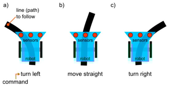
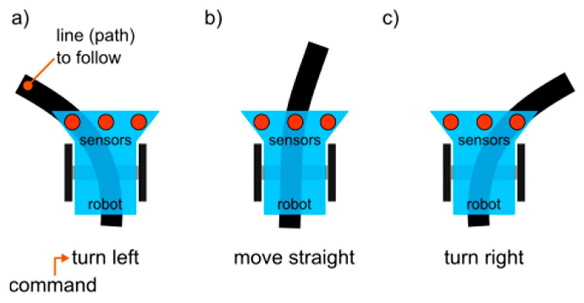
Figure 1.
Control principles for typical line-following, 2-wheeled robot showing situations resulting in (a) turn left, (b) move straight, (c) turn right commands.
Due to the very simple control rules, this task is often presented as one of the first during robotic classes for students or as the introduction to mobile robotics for children. There are various types of line-following robots, starting from toys, through various enthusiast-level robots, advanced “racing” robots for line-following competitions [9,10,11], up to professional, industry-grade constructions. For example, some of the AGVs (Automated Guided Vehicles) in factories and logistic centres also utilise line-following principles in their control systems [12]. The line to follow might be a visual line painted or embedded (e.g., electrical or magnetic wire) in the floor or ceiling. Line detection and following also play an important role in autonomous driving systems applied in road cars [13,14]. In order to detect the line, various types of sensors might be used, for example, light reflection sensors, infrared sensors, magnetic sensors, video cameras, and others. Even though there are already plenty of line-following robots on the market, there are still new constructions [15,16] and new control algorithms developed: for example, ones based on fuzzy sets [17], the dynamic PID algorithm [18], AI swarm algorithms [19], vision systems combined with infrared sensors [20], and others.
Although most of the line-following robots are ground vehicles that operate in a 2D space, there are also some implementations of this principle for industrial robots and for aerial robots. For example, in [21] the artificial Double Deep Q-Network was applied for performing the path-following task using an articulated robot. The network was trained to follow a path drawn on a flat surface and observed locally by a camera mounted on the robot arm. The achieved path tracking error was below 1 mm. In the paper [22], a system for extracting the features of and tracking a weld joint was presented. It utilised a laser scanner to detect the path defined by the contact line of two metal elements to weld. However, the system was tested only on a straight, flat (i.e., defined in the 2D space) path. An example of the application of line-following principles in aerial robotics is robotic competitions [23], where a robot equipped with a camera must reach the end of a line that is drawn on the floor. Another example is the application of UAVs (Unmanned Aerial Vehicles) for chemical spraying in agriculture [24], where a robot equipped with a camera detects lines of crops and flies along them. Another example is [25], where a UAV was used for pipeline inspections and the data from the vision system processed using a Convolutional Neural Network were used for navigating the drone along the pipe. However, the system was tested only for pipes lying flat on the ground and the UAV was flying at a fixed altitude. It must be noted that, even though these robots fly in a 3-dimensional (3D) space, they still follow a line detected on the ground, i.e., defined in a 2D space, at a constant flight level. There are very few attempts to implement the line-follower principle for following a path physically defined in a 3D space. One such example is [26], where a UAV is designed for an aerial power line inspection. It tracks the powerline using a LiDAR sensor. Another example, described in [27], is also a UAV for power line inspection. In this paper, the arrangement of the line to follow is extracted from the camera image of the aerial powerline. To keep the UAV centred and oriented with the lines, the PID controller tuned with the fuzzy logic algorithm is used. Unfortunately, the performance of the algorithm was tested in simulation environments only. It is also noted that it will need to merge the information acquired by the camera with laser sensors in order to determine the distance of the UAV from the followed power line. In [28], the control of an AUV (Autonomous Underwater Vehicle) for underwater cable tracking is presented. The tracking of a cable buried in the seabed is achieved by magnetic field sensing. Thanks to this, not only can the direction of the tracking be obtained but also the distance from the cable can be maintained. However, the control algorithm does not take into account the presence of environmental disturbances (e.g., water currents) or obstacles (e.g., underwater sand-waves). The authors admit that a more advanced algorithm enabling more than just fixed AUV-to-cable distance maintaining in the 3D space must be developed. The need for developing the AUV for monitoring underwater structures, including pipes and cables, as well as some preliminary design of such a platform is also presented in [29].
From the literature review, it appears that vision processing techniques have a high capability for detecting objects and shapes, including lines and paths, but they lack sufficient information on the scene’s depth. Thus, they must be accompanied by some distance measurement techniques, for example, LiDARs, radars, 3D cameras, or stereo vision, which increases costs and computational power demand. It also introduces problems with the synchronisation and fusion of data from various systems [30]. An additional drawback, in the context of the task described further in this paper, is that some types of sensors have limited capabilities in terms of detecting objects located close to sensors (i.e., closer than a few centimetres).
It must be underlined here that there are a lot of works on the subject of 3D path-following or tracking, with a great variety of methods being applied [31,32], but the 3D “path” is usually defined as a set of the robot’s configuration states, including coordinates to be reached or passed by the robot on its way. These coordinates are just points defined in some space. There is no physical line to be followed. This is a very different case from the one that will be described in this paper.
The aim of this work is to enable continuous, step-by-step control of robot incremental motion following a path in 3D space. This is obtained based on the classic line-follower concept, and the control rules are developed in order to allow an articulated, 6DoF (Degree of Freedom) industrial robot to follow the physically existing path defined in 3D space. The literature on this defined problem is, to the authors’ best knowledge, very limited.
Nevertheless, a somewhat similar problem was investigated in [33], where the shape of a physically existing line was detected using a camera and the articulated robot learned how to move along it using reinforcement learning. However, even though the line was defined by a hose placed in the robot’s space, the path was flat, i.e., this was in fact a 2D problem. Moreover, the solution was not calculated step by step and, as the path was analysed globally, it belongs to the global planning methods.
In [34], a very wide review of vision methods for automatic robotic welding is provided. Welding involves accurate control of the robot effector movement along a path that is defined by two adjacent, contacting elements. This is a problem that may appear similar to tracking a 3D path. However, the path is not detected directly but is rather described by the intersection of adjacent surfaces or by a groove on the surface. The presence of adjacent surfaces makes the locating of the path easier, and in the case of groove detection, closer to a 2D line-following problem. Most of the methods described in [34] offer a weld seam tracking accuracy between 1 and 0.1 mm. In the most accurate solutions, vision systems are accompanied by laser scanners.
Another publication that presents a similar task is [35], where an industrial robot was controlled by an Artificial Neural Network trained to follow an arbitrary path drawn by a human demonstrator on a 3D surface. Line detection and tool orientation were extracted from the image obtained from the camera placed on the robot’s effector. A laser beam was used to mark the tool orientation relative to the path on the surface to help extract it from the image obtained from the camera. Three different reinforcement learning algorithms were compared in terms of path tracking accuracy, with the Proximal Policy Optimisation reinforcement learning algorithm achieving a maximum tracking error of 4 mm and mean error of 0.2 μm.
Contrary to the majority of the publications, this paper presents a method for following a path that is physically defined in a 3D space. The path position is detected using a simple tool held by an industrial 6 DoF robot. The tool is equipped with six low-cost Time-of-Flight (ToF) sensors. The task to be performed is to move the robot arm with the tool along the path from the start to the finish point, without a collision with the path. Only the start position is known a priori, before the start of the whole process, so the path position and orientation must be detected, and proper robot arm movements must be calculated on-line, as the following of the path progresses.
2. Materials and Methods
2.1. General Description of the Proposed Solution
The general concept of the algorithm is to extend the classic idea of the line-follower into a 3D space. The path shape is defined using a hose mounted inside the robot’s workspace. The path’s position is detected by the sensors placed on two perpendicular arms of the path detection tool (Figure 2). Thanks to this, the path’s existence may be detected in points located at the sensors’ line-of-sight intersections. However, this allows for path detection only inside the 2D space of the detection tool. In order to detect the path’s orientation in the 3D space, the robot moves the tool by a small amount and performs a second detection. Thanks to this, it is possible to calculate how the sensing tool should be moved along the path to the next position to perform the next detection. Then, the process is repeated, taking into account the tool’s new (now current) position, and its previous position. When moving to subsequent positions, it is also important to always keep the sensing tool oriented perpendicular to the path. It must also be underlined that it is assumed that the path is not placed flat but bends in various directions in 3D. The details of the proposed solution are presented in the following subsections of this chapter.
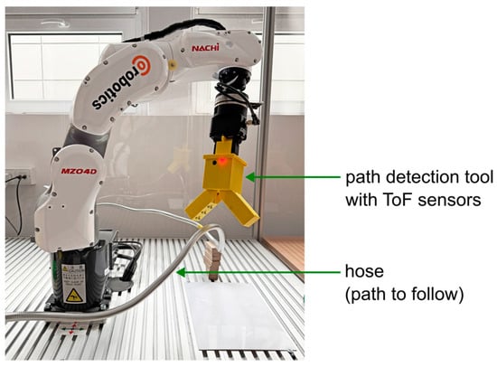
Figure 2.
Robot holding path detection tool during the path-following.
2.2. Detected Path Position Calculation
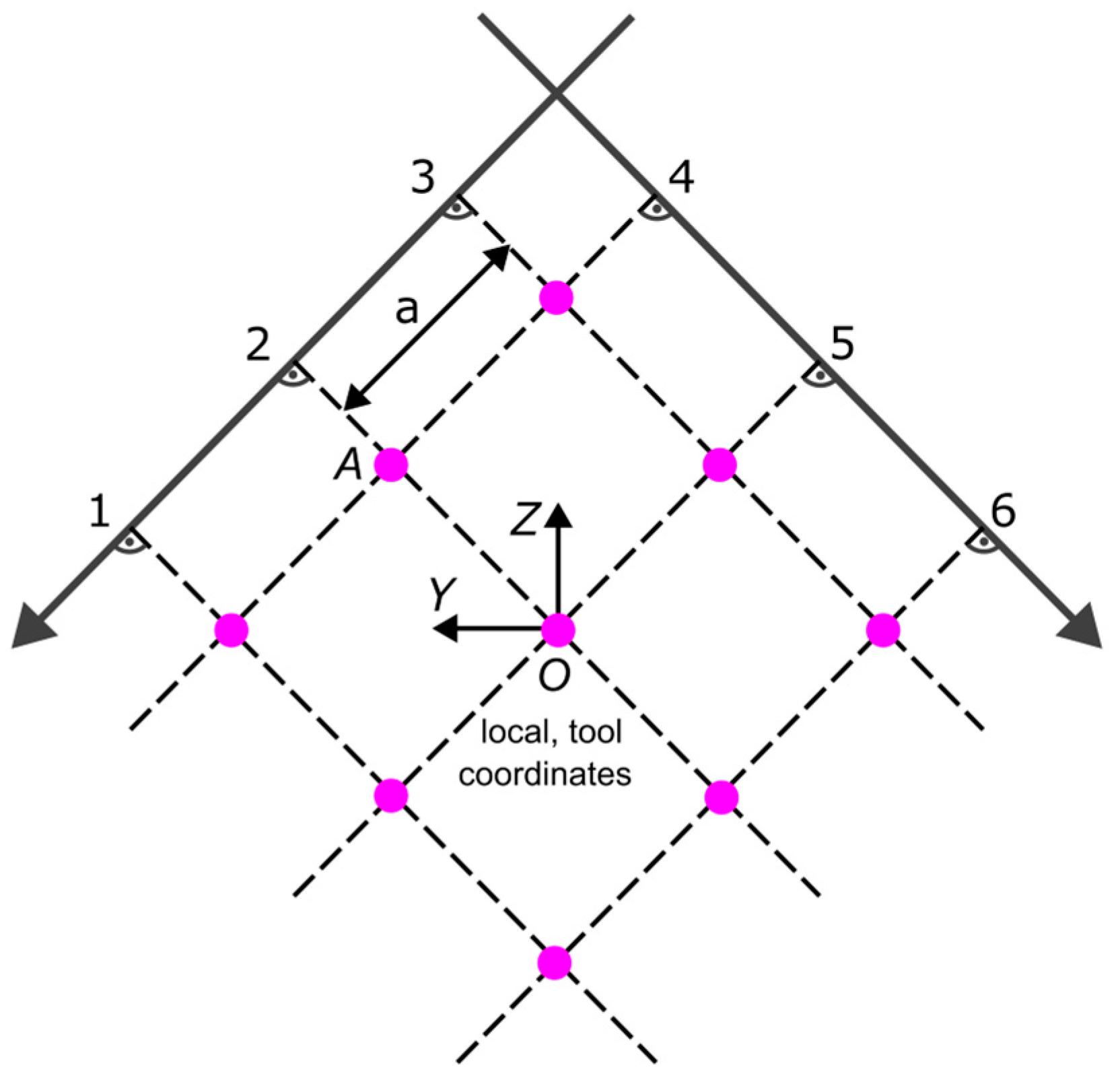
Figure 3 presents an exemplary path detection tool with 6 sensor placements and the detection points of the path detection tool marked. The current tool position is always known, i.e., it is calculated based on the gripper global position returned by the robot controller. The centre of the tool’s coordinate system (O, tool position) is located in the middle of the detection field. It lies at the intersection of the lines of sight associated with the two central sensors (No. 2 and 5 in Figure 3). The Y and Z axes lie in the tool plane, while the Z axis is perpendicular to this plane. The sensor spacing is .
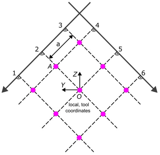
Figure 3.
Path detection tool schema showing ToF sensors (1–6) placement, sensor separation a, and locations of detection points (purple circles), e.g., point A is the detection point at the intersection of the lines of sight of sensors 2 and 4.
Each of the intersection points of the sensors’ lines of sight in the global system can be determined by knowing the position of the tool and its orientation in the form of Euler angles. Euler angles determine the orientation of the local tool coordinate system relative to the global system (located in the robot base). The first stage of the process of calculating these points is to determine the rotation matrix of the local tool system:
where —rotation angle around the X axis (roll); —rotation angle around the Y axis (pitch); —the angle of rotation around the Z axis (yaw); —rotation matrices around individual axes, respectively, X, Y, Z; and —tool rotation matrix.
The position of a point in the global coordinate system, knowing its position in the local coordinate system, can be determined using the following formula:
where —the desired point position in the global system; —the centre of the local coordinate system; and —the vector of the position in the local coordinate system (the vector between the centre of the local coordinate system and the position of the desired point in this system).
The general formula for calculating detection point positions (intersections of sensors’ lines of sight) is
where —the intersection of sensors’ lines of sight in the coordinate system of the robot base; —unit vector; and —the distance between the centre of the local coordinate system and the desired point i.
The next step is the calculation of the middle point based on the set of points where the path was detected, because it is possible that the path is detected in more than one point simultaneously. This is calculated according to the following formula:
where —the midpoint, i.e., the point where the followed path is assumed to be; —coordinates of points where the path was detected; and —the number of points where the detection occurred.
In some cases, it is also possible that the path is not detected at all, for example, when the path is located between the sensors’ lines of sight. In such case, , which means that it is assumed that the path is in the middle of the detection tool and the robot should continue in the previously calculated direction. This is performed in order to deal with detection errors caused by the limited special resolution of the detection tool. It is also assumed that by moving forward, the path will eventually be again.
2.3. Calculation of the Next Tool Position
To determine the next position where the detection tool should be moved by the robot, it is necessary to calculate the appropriate vector (Figure 4). In the previous section, how to designate the point that represents the detected path position was presented. Knowing the position of this point, the next step is to determine the vector between this point and the position of the detection tool (point ).
where —point coordinates; —point coordinates.
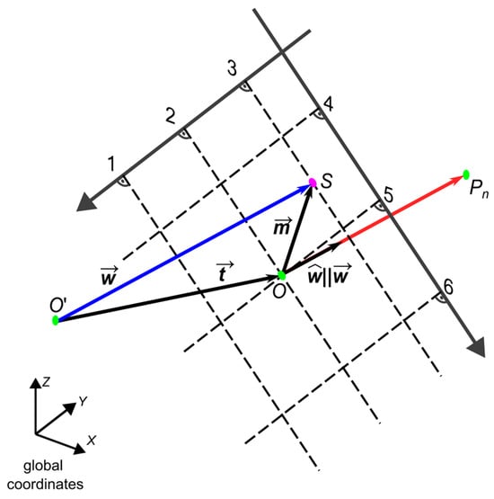
Figure 4.
The vector and its component vectors and location of (next tool position) point in the global coordinate system; is the unit vector parallel to . Other symbols: —tool displacement vector; —detection tool centre in the current position; —detection tool centre in the previous position; and S—detected path position.
Additionally, the tool displacement ( vector) from the position where the path was detected for the last time (point ) must be calculated:
It must be noted that the position is not always the last (previous) tool position. This happens when the path is not detected by the tool. In this case, it is assumed that the path is located between the sensor’s lines of sight, and it should be detected again in one of the next moves, so the tool is moved ahead in the previously calculated direction but the point used in (10) is still the one obtained when the path was detected the last time. Apart from handling temporary path loss, this also helps to react appropriately to path bends, depending on how sharp they are.
After summing up both vectors and , the resultant vector is obtained (11), which is the vector needed to determine the next tool position. Then, the vector must be normalised (12). The resulting unit vector allows the determination of the new position shifted by a given distance d (Figure 4).
where —vector between and S points; —unit vector; —tool displacement distance; and —next tool position.
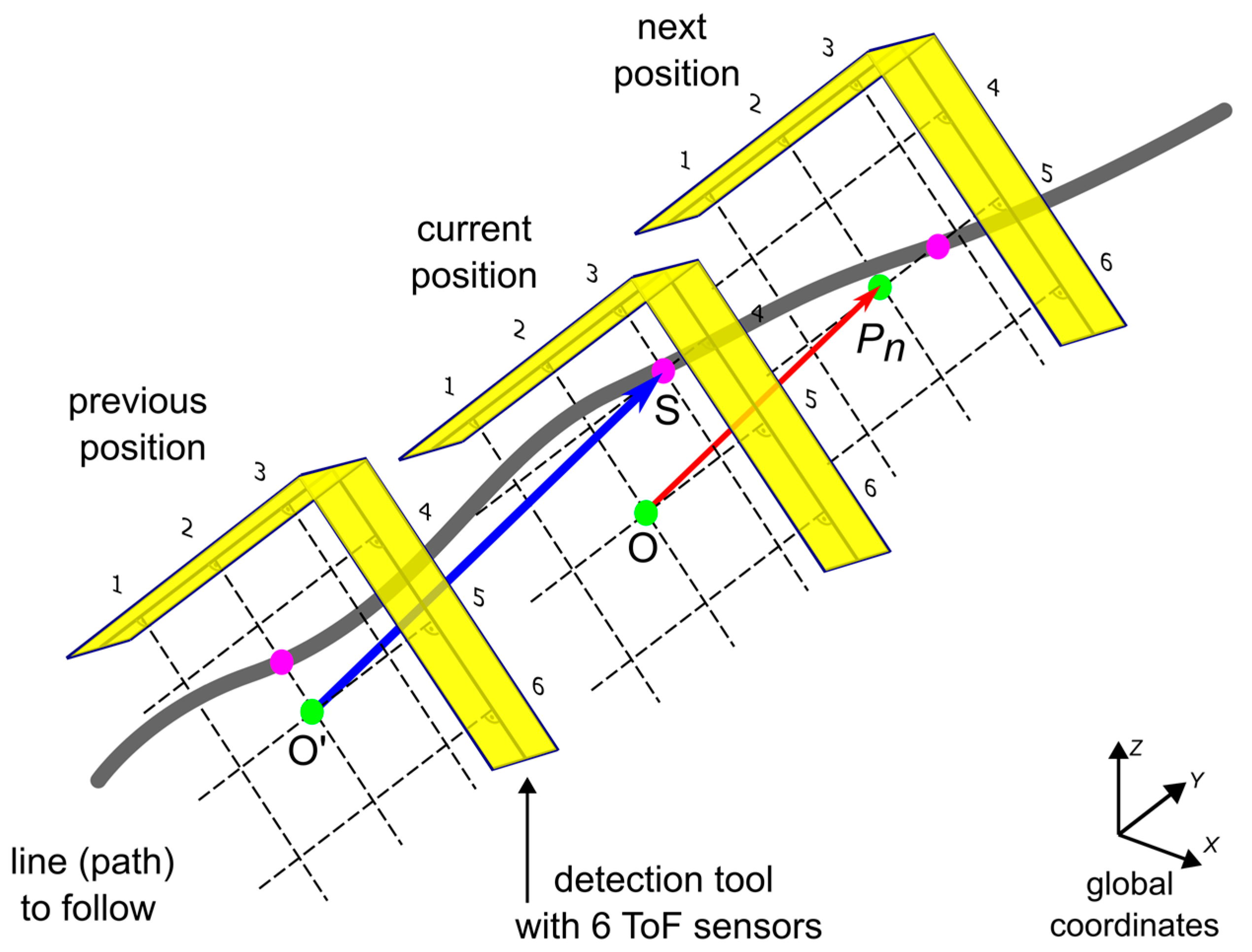
Figure 5 presents the general scheme of the path-following, showing 3 consecutive positions of the path detection tool.
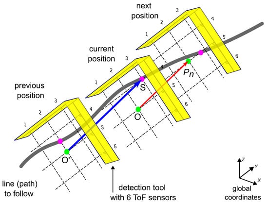
Figure 5.
Three consecutive positions of the detection tool during path-following. Symbols: —detection tool centre in the current position; —detection tool centre in the previous position; S—detected path position for the current detection tool position; and Pn—calculated next tool centre position, 1…6—ToF sensors.
An exception to the rules described above is the situation when the midpoint is placed in the tool centre (point ). In this case, the next position is calculated based on the vector normal to the tool plane (tangent to the X axis of the tool).
This is caused by the fact that tool rotation is calculated separately (which is described in the next section), and even though the path is in the tool centre, the vector and normal vector may differ.
2.4. Calculation of the Tool Rotation
The detection tool detection field, which lies in the Y and Z axes (in the local tool coordinate system), should be oriented perpendicularly to the path. In this orientation, it is easiest to detect the path and to avoid tool collision with the path. Therefore, the orientation of the tool is as important as the position in the Cartesian coordinates of the tool and must be determined on-line. The adopted method of determining Euler angles, analogous to the process of determining the sequential tool positions, is based on the calculation of the vector that defines the new orientation of the axis of the tool’s coordinate system. Thank to this, two rotation angles can be defined, and the third rotation angle (rotation around the axis) is imposed. This tool orientation vector differs from the vector used for position calculation because it is possible to modify its parameters. By introducing this approach, it is possible to tune the algorithm and achieve smoother path-following.
To obtain the tool rotation vector, the vector normal to the plane lying in the Y and Z axes of the local tool coordinate system must be determined:
where —unit vector oriented along axis of the tool coordinate system; —vector normal to the tool plane.
Using the previously determined vector, the tool orientation vector may be calculated as follows:
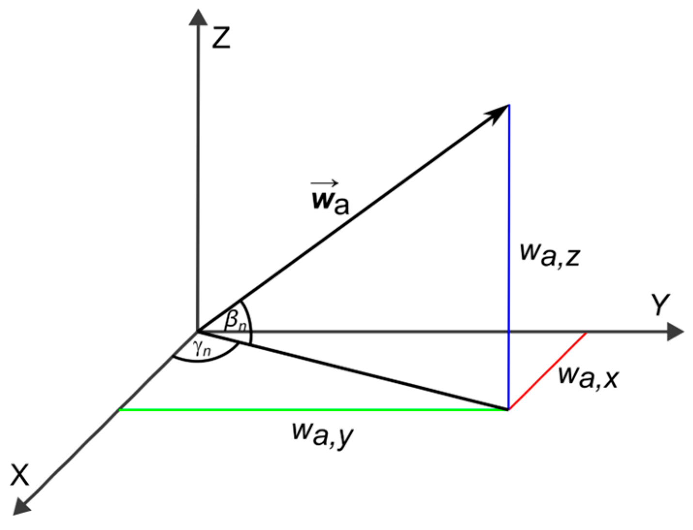
where —vector’s modification parameters, experimentally adjusted during tests; —orientation vector (Figure 6).
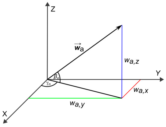
Figure 6.
The vector with its components, , and two rotation angles that can be determined on the basis of this vector: and .
If, in Equation (17), parameter a is set to the scalar value (i.e., length) of , the rotation is indirectly proportional to the path arc radius. When the radius is high, the path bend is small and there can be a few subsequent steps when the path is not detected by the tool. When the radius is low, the path bend is high, and the path is detected frequently. This means that normal vector length is dependent on the distance between the subsequent path detection positions. Parameter b, which is manually set constant with a value below 1, acts as tool rotation reduction coefficient. This prevents too high tool rotations when the path is detected in two subsequent positions in different detection tool points. In such a situation, the vector may be much longer than vector . As a result, the orientation vector may be oriented almost parallelly to the detection tool plane, i.e., it indicates very high rotation. This may cause the collision of the detection tool with the path and also results in high oscillations of the detection tool around the followed path. The reduction of the vector prevents both situations. Thanks to this, smoother path-following is achieved, which, in turn, results in better path detection effectiveness. The only drawback of this solution is that in the case where the path has a low radius bend, the tool cannot be turned to the proper orientation in one step. In this case, the bend is negotiated in a few subsequent steps.
The trigonometric relationships and the Pythagorean theorem result in the following:
where —new rotation angle around the Z axis (yaw); —new rotation angle around the Y axis (pitch).
The minus sign in Equation (19) results from the use of a right-handed coordinate system. In such a system, the positive angle (pitch) corresponds to the counterclockwise rotation around the Y axis. In case the component of the vector is positive, it corresponds to a clockwise rotation. For this reason, the expression must include a minus sign to conform to the convention. As the result, using the arctangent function, new tool rotation angles can be determined:
and a constant value assigned to the angle of rotation around the X axis (roll):
Figure 7 presents the summary of combining calculations of both tool rotation and the next tool position.
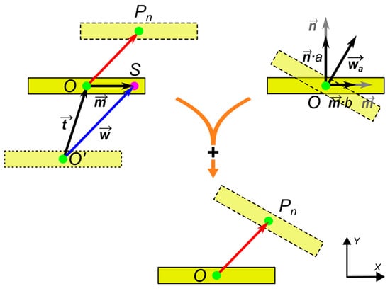
Figure 7.
Example of combining the next position and tool rotation; detection tool seen from the top. Symbols: —detection tool centre in the current position; —detection tool centre in the previous position; S—detected path position for the current detection tool position; Pn—calculated next tool centre position; vectors , , , , and and a and b constants are described in the text.
2.5. Determining the Position of the Detection Tool Based on the Position of the Gripper
In previous sections, it was assumed that the position and orientation of the effector (detection tool) are known. However, during experimental tests, when the robot controller was queried for actual robot position, the gripper position was returned, because this is how the effector was defined in the robot controller. Of course, it is possible to define a new effector in the robot software, but it was decided to determine the position of the tool on the control computer side, i.e., in the Mathworks Matlab version 2023b (Mathworks, Natick, MA, USA) environment. This solution was selected to facilitate the incorporation of the tool geometry modifications, anticipated during project development, into the algorithm and to discard the need for adjusting the tool definition in the robot controller if any change in the tool is made. Additionally, thanks to this approach, the whole algorithm is more robot-independent, i.e., there are no configuration changes to be made in the robot controller settings.
The tool coordinate system is shifted (in relation to the gripper system) along the Z axis of the gripper by the distance . Its orientation in relation to the gripper system can be described by the following angles: —rotation angle around the axis (roll); —rotation angle around the axis (pitch); and —rotation angle around the axis (yaw). During the experiments, these angles were as follows: roll , pitch , and yaw
In order to find the position of the tool, the first step is to determine the rotation matrix of the gripper system with respect to the global coordinate system. Using the relationships describing the rotation matrices around individual axes Equations (1)–(3), the rotation matrix of the gripper system has the following form:
where , , —gripper rotation angles (roll, pitch, and yaw); —gripper rotation matrix.
The tool coordinate system is shifted along the gripper Z axis in the positive direction. Knowing the position of the centre of the gripper coordinate system, it is possible to determine the position of the centre of the tool system using Equation (5). The formula for the position of the centre of the tool system takes the following form:
where —gripper coordinate system centre.
Next, the orientation of the tool coordinate system relative to the global coordinate system must be determined. First, the rotation matrix of the tool system in relation to the gripper system is determined, again using Equations (1)–(3):
where —rotation matrix of the tool’s coordinate system relative to the gripper’s coordinate system.
Using matrices and , it is possible to determine the rotation of the tool coordinate system in relation to the global coordinate system (i.e., to the robot base):
where —rotation matrix of the tool coordinate system relative to the coordinate system of the robot base.
On the basis of the determined matrix, , it is possible to determine the orientation of the tool in the form of Euler angles. According to [36], however, there is always more than one possible solution and the selection of angles is arbitrary, because they result in the same orientation of the system.
3. Results
3.1. Experimental Setup
In order to prove the reliability of the proposed algorithm, experimental tests were carried out using the industrial, articulated, 6DoF robot Nachi MZ04D (Nachi Fujikoshi Corp., Tokyo, Japan) with a Nachi CFD controller [37]. The maximum load capacity of this robot is 4 kg, and the maximum reach of the flange is 541 mm. The robot is equipped with a Gimatic MPLF 2550 (Gimatic, Roncadelle, Italy) electric gripper and Schunk FT-AXIA 80 (Schunk, Lauffen/Neckar, Germany) force and torque sensor, which was installed on the robot but was not used during this research. The path to follow was set up using a shower hose (20 mm diameter) with a 3 mm copper wire inside, so that the hose retains its position when setting the path. The hose was attached at both ends to the worktable with metal brackets. Additionally, it was supported with some blocks and boxes to obtain the desired path, but these supports were placed outside the path-following zone.
The robot was enclosed in a safety cell with the dimensions 1250 × 1250 × 1250 mm. In the robot controller software, the virtual safety walls were set to −550 … +550 mm in the X axis, −550 … +550 mm in the Y axis, and +5 … +inf mm in the Z axis. Similar boundaries were defined in the IK solver settings utilised in the path-following algorithm. The robot was placed in one of the didactic laboratories of the Gdansk University of Technology, which ensures stable environmental conditions (room temperature around 21 °C, humidity around 30%, appropriate lighting).
The path detection was provided thanks to the specially designed detection tool (Figure 8). It consists of a box with communication electronics and six ST Microelectronics VL6180X (ST Microelectronics, Plan-les-Ouates, Switzerland) infrared Time-of-Flight sensors [38] placed on two perpendicular arms, three sensors per arm. These sensors can detect objects at a distance from 0 to 100 mm away from the sensor. The measurement accuracy is not explicitly provided in the datasheet; however, it contains the following information: measurement noise up to 2 mm, temperature-dependent drift 9 mm, and voltage-dependent drift 3 mm. All of the sensors were calibrated before use according to the procedure described by the manufacturer. Nevertheless, it must be noted that range (distance) measurement data are not directly used for path detection. Only the presence of the path in the detection zone of a sensor is used, not the exact distance value. Experimental verification proved that this is sufficient if only a small part of the path (hose) lies in the sensor’s detection sight, as its detection is stable. It must also be noted that the detection field of each sensor is not a narrow, straight line but a cone with a vertex located in the sensor position and 25° vertex angle. Because of this, as sensors are separated by 22 mm (which makes 31 mm when considering the grid diagonal), and the hose diameter is 20 mm, it is common that the path is detected by more than one sensor. In such situations, path position is calculated using Equation (8). This means that the overall accuracy of the path centre detection is not worse than ±16 mm.
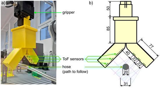
Figure 8.
Path detection tool used during experimental verification: (a) view of the real tool in the robot gripper placed over the path to follow; (b) main tool diameters.
Data from sensors were read by an ST Microelectronics STM32G431 microcontroller (MCU) on an STM32 Nucleo board via I2C bus and then sent to a personal computer (PC). The communication between the tool and a control algorithm running in Matlab on the PC was provided via a wireless Bluetooth 4.0 BLE connection. The tool is independent from the robot, i.e., it is grasped by the robot’s gripper at the beginning of the program and then moved to subsequent positions, but there is no connection (i.e., no wires) and no direct communication between the tool and the robot or the robot controller. For the designed detection tool, the distance (Equation (24)) was 159.7 mm.
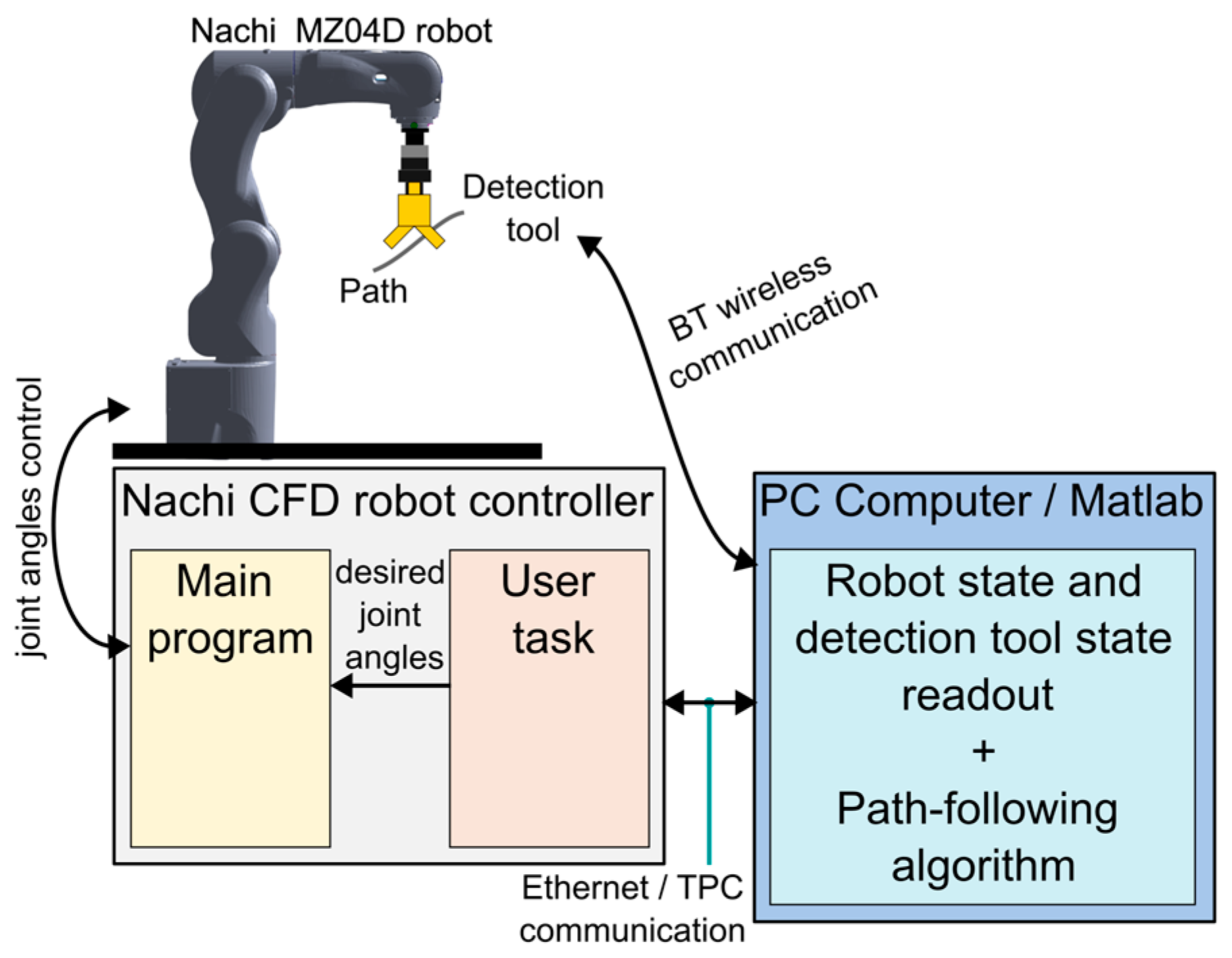
The software architecture of the whole system is presented in Figure 9. Data from the detection tool are read by the control program running in Matlab. This program, based on the current and previous detection data, calculates the next detection tool position, i.e., where the robot arm should be moved. Calculated robot joint positions are sent (via Ethernet) to the robot controller. On the controller, there are two programs running, the main one and the so-called User Task [39]. User Tasks are additional programs that can run in parallel with the main program. In the presented case, the User Task developed for the purpose of this research was responsible for two-way communication with the PC. It must be noted that although the User Task can perform various tasks associated with the robot control, it cannot contain commands that execute the physical moves of the robot arm. Moves can only be performed by commands included in the main program. Due to this, the User Task writes joint angles received from the PC to internal registers of the robot controller and the main program reads them and moves the robot to the desired position. Additionally, the developed User Task can also return current robot position as joint angles or Cartesian coordinates, operate the gripper, and perform some additional robot settings. Communication between the Nachi CFD robot controller and PC is provided via Ethernet and TCP protocol.
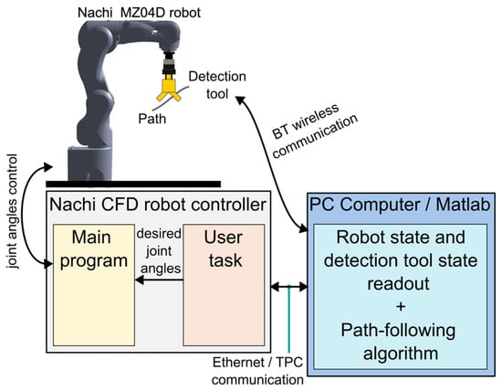
Figure 9.
General software architecture of the presented system.
3.2. Algorithm Implementation, Constraints, and Supporting Solutions
The path-following procedure schema is presented in Figure 10. The process starts with the initialisation of the communication between the program running on the PC in Matlab and the robot controller as well as the detection tool. Once all hardware elements are connected, some initial moves of the robot are performed. These are detection tool pick-up and moving to the start position located over the path. Then, in the loop, for each stage the following steps are repeated for a given number of iterations:
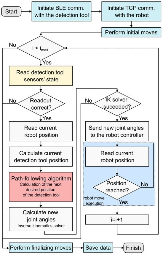
Figure 10.
Path-following algorithm schema.
- Read sensor data and interpreting these data:The measurement field of the detection tool is represented as a 3 × 3 array (sensor array). Path detection is possible at nine points that are located at the intersections of the sensors’ line of sight. Each of the points is represented by one element of the sensor array. The matrix rows represent the sensors located in the left arm of the path detection tool (sensors 1–3) and the columns represent the sensors in the right arm (sensors 4–6). The path is marked as detected at a given point when its presence is signalled by two sensors whose fields intersect in this point. Additionally, if the path is detected too close or too far from the sensor it is marked as a detection error to prevent unambiguous data input to the path-following algorithm. A detection error is not treated as a wrong readout. In such a case, the algorithm continues as if the path was not detected in this step and calculates the next step based on the last successful readout (the O’ point of the last step when the path was detected is used).
- Read the current position of the gripper from the robot.
- Calculate the effector’s (detection tool) current position and orientation based on the position of the gripper using Equations (23)–(25).
- Perform path-following algorithm step:Calculate the effector’s new position based on its current and previous positions and detected path position. First, the detected path position is calculated using Equations (1)–(8). Then, the next tool position and rotation is calculated using Equations (9)–(14) and (15)–(22). It must be noted here that according to the detection condition, a “long” or “short” step is performed (according to the value of the variable d in Equations (13) and (14)). A “short” step is performed when the path is detected only in the central point of the detection field or when it is not detected by any sensor. In all other cases, a “long” movement is performed. This is to prevent an insufficient correction of the detection tool position when the path trajectory bends or losing the path when moving straight ahead. Moreover, in some cases, due to the algorithm’s response to detecting a path in a position other than the centre of the detection field, the calculated tool rotation may have a high angle value (see Section 2.4). This has a negative impact on the smoothness of the motion along the path and may also cause the loss of path detection. Rotation reduction is accomplished by reducing the length of the vector. It is multiplied by a constant parameter (named b in Equation (17)), which should have a value greater than 0 and less than 1. This reduction may, however, cause the situation where the tool rotates by a smaller angle than is needed. Fortunately, in such a case the path-following algorithm will recognise in the next iteration that the path is still positioned on the edge of the detection field and, in order to follow the path, it must be rotated again. Eventually, the algorithm corrects the tool orientation in a few subsequent movement steps.
- Calculate inverse kinematics (IK):The IK function calculates the articulated variables of the robot based on the detection tool position and orientation determined by the path-following algorithm. To calculate IK solution, the Matlab generalised IK object [40] is used, which internally uses the Broyden–Fletcher–Goldfarb–Shanno (BFGS [41]) gradient projection algorithm solver. As a starting point for the solver to find the solution for the next position, the previous robot position is used. There are also some additional solver constraints applied that limit the robot body elements to stay inside safety cell, force the solver to prefer the downward tool orientation, and limit maximum tool rotation around its axes to less than 90° to prevent tool reversal, which will cause a collision with the path.
- Send new joint positions to the robot controller.
- Execute robot move:Robot moves are executed with an arbitrary chosen constant speed. Read, in a loop, current robot position and wait until it reaches the assigned position.
Once the algorithm performs the desired number of iterations, the finalising moves are executed, i.e., the detection tool is stored back in its holder, the robot moves to the safe position, and program execution logs are saved. During the development of the software for communication between the PC and the Nachi robot controller, a few minor software elements and information on Nachi MZ04 robot performance provided in [42] were employed.
The full software developed for the purpose of this paper is available as the Supplementary Data provided as [S1]. This includes the main program for the robot controller, the User Task for the robot controller, the STM32 project for STM32G431 microcontroller, and the Matlab implementation of the path-following algorithm.
3.3. Experimental Verification
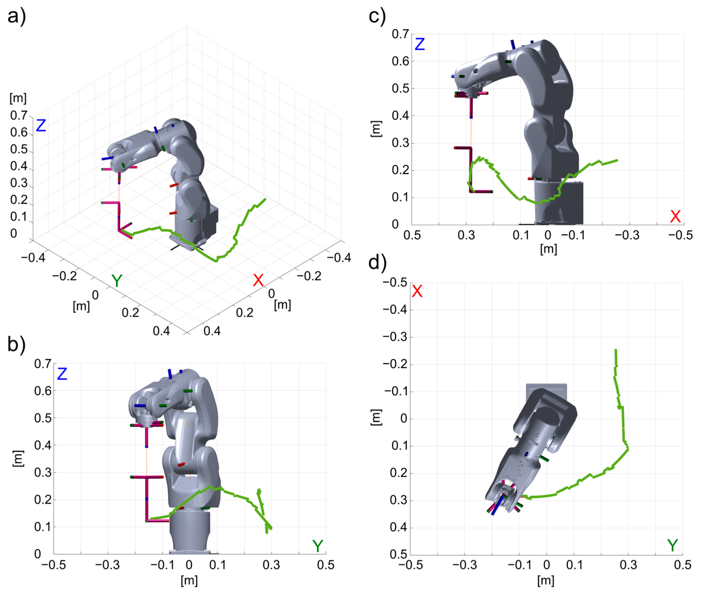
To demonstrate the effectiveness of 3D path-following using an industrial robot controlled by the developed algorithm and the proposed path detection tool, tests were performed for four different path settings. Path 1 was tested twice and then tests for paths 2, 3, and 4 were performed. In each presented case, the task was successfully accomplished. Below, views of the recognised paths are visualised. In each figure, the robot is presented in the initial position, and the path is presented as a green line. Note that the figures show path positions as they were detected by the path detection tool and as they were represented in the algorithm. These are not the actual, real locations of the path but are close to them. Additionally, photos of some selected positions obtained by the robot during the program run are also presented. A full view of each run is presented in the video available as the Supplementary Data provided as [S2].
3.3.1. Path 1, Run 1
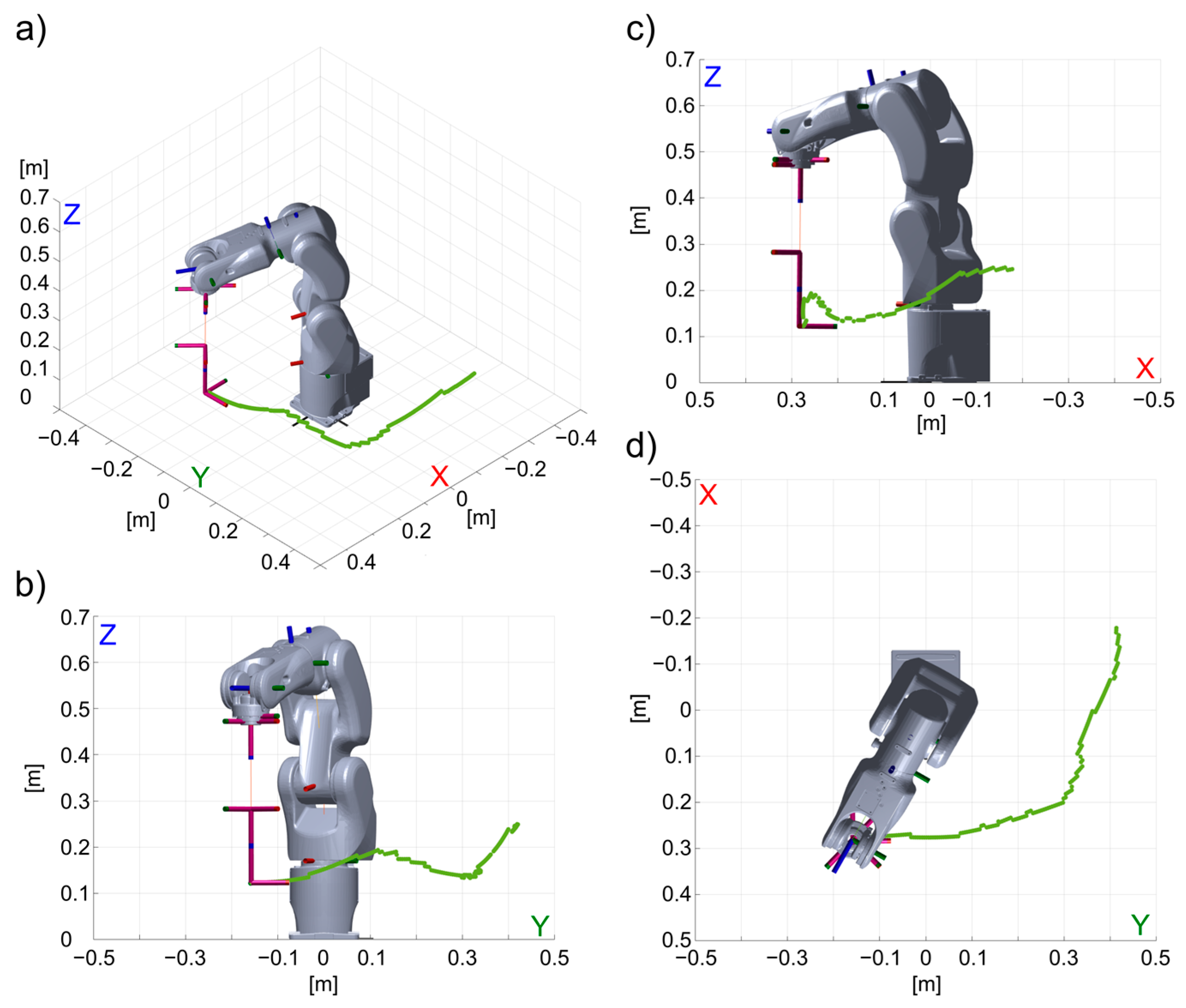
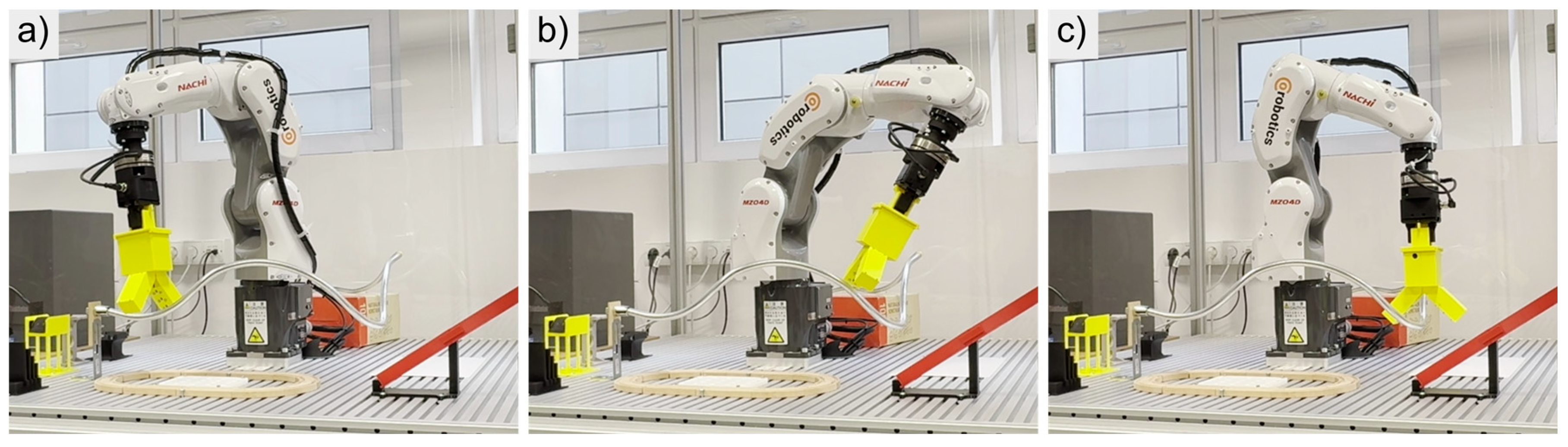
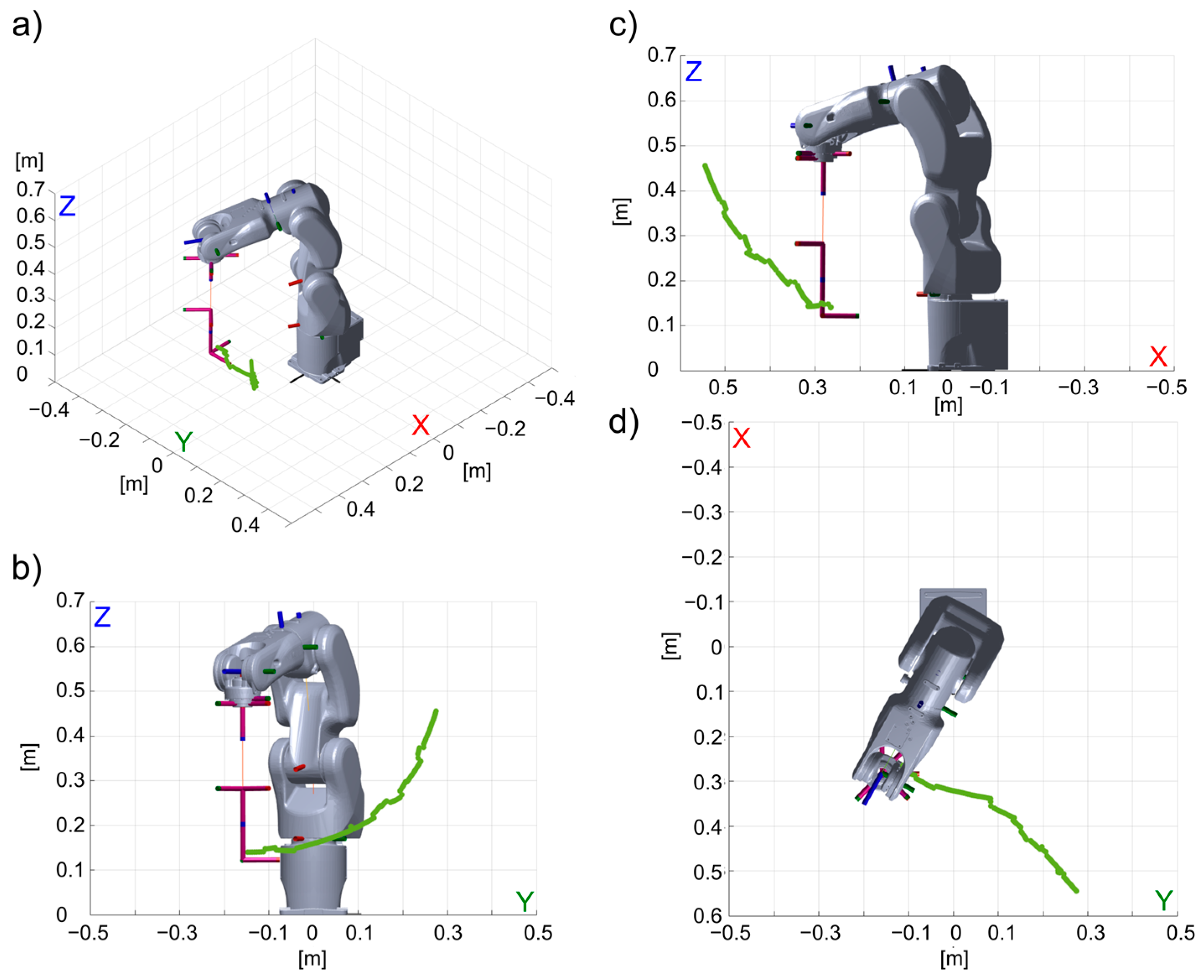
The first path was composed with some up and down bends with moderate arc radiuses. This path was successfully followed by the robot. Figure 11 presents four views of the detected path and Figure 12—three selected examples of robot positions obtained during path-following.
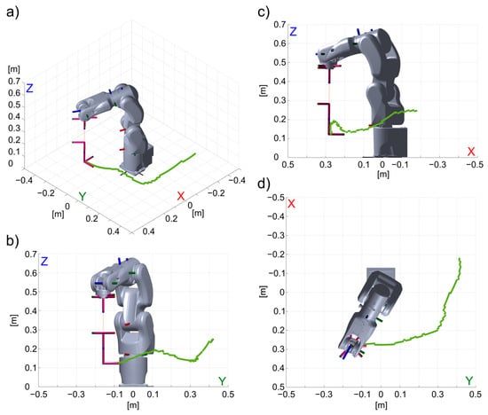
Figure 11.
Path 1, run 1—path (green line) detected by the detection tool (a) isometric view, (b) front view (YZ plane), (c) side view (XZ plane), and (d) top view (YX plane).

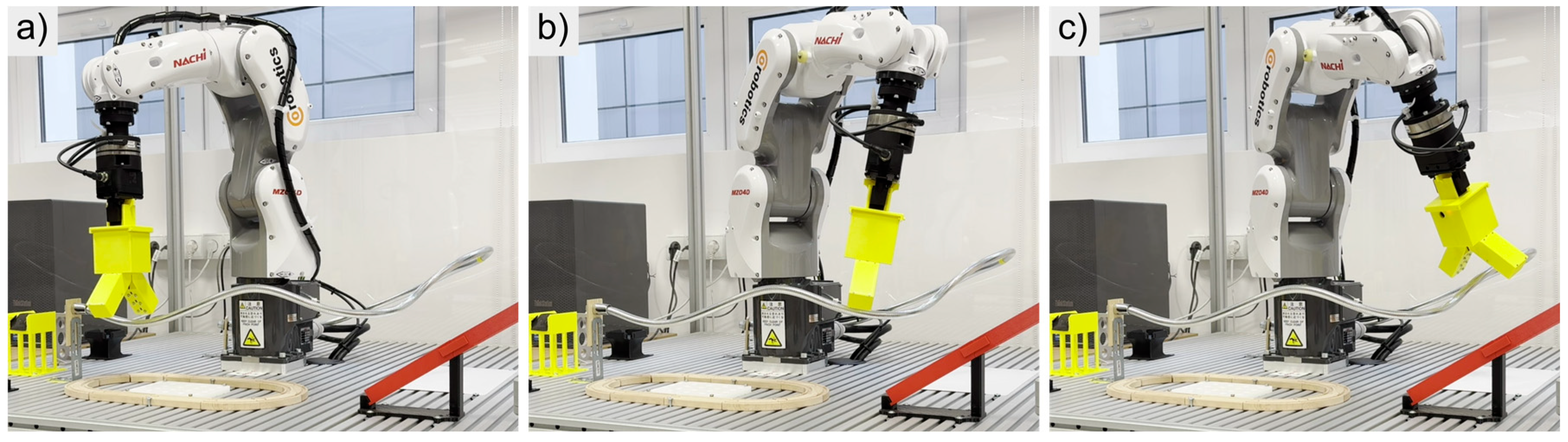
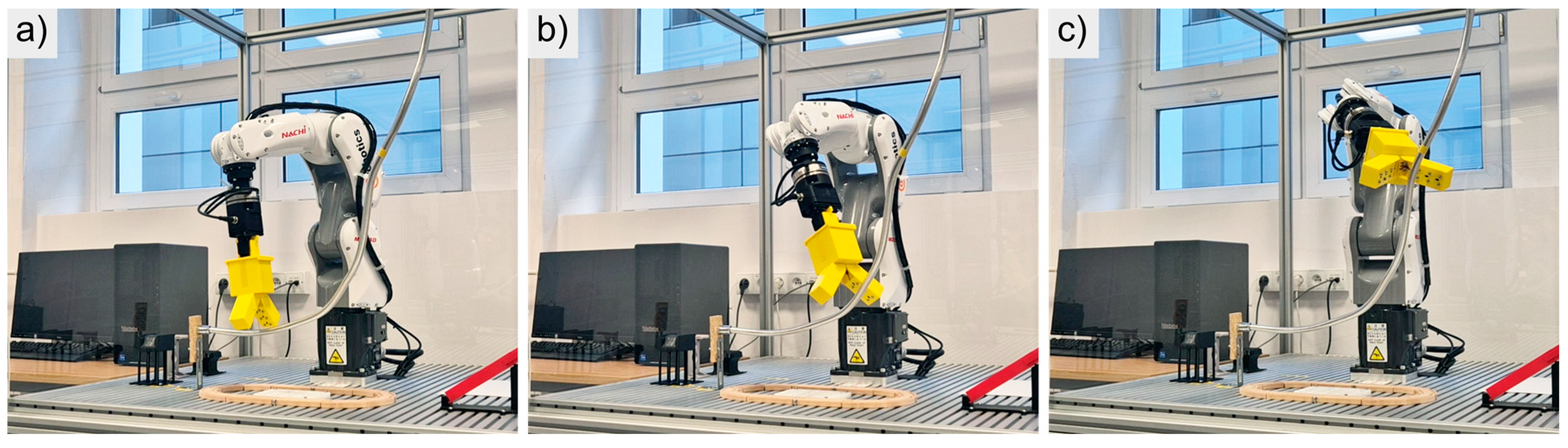
Figure 12.
Path 1, run 1—(a–c) three selected examples of robot positions obtained during path-following; full video available as Supplementary Material [S2].
3.3.2. Path 1, Run 2
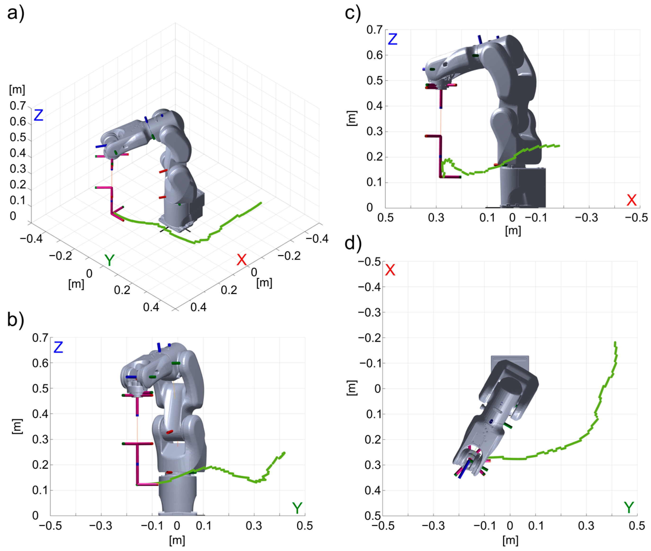
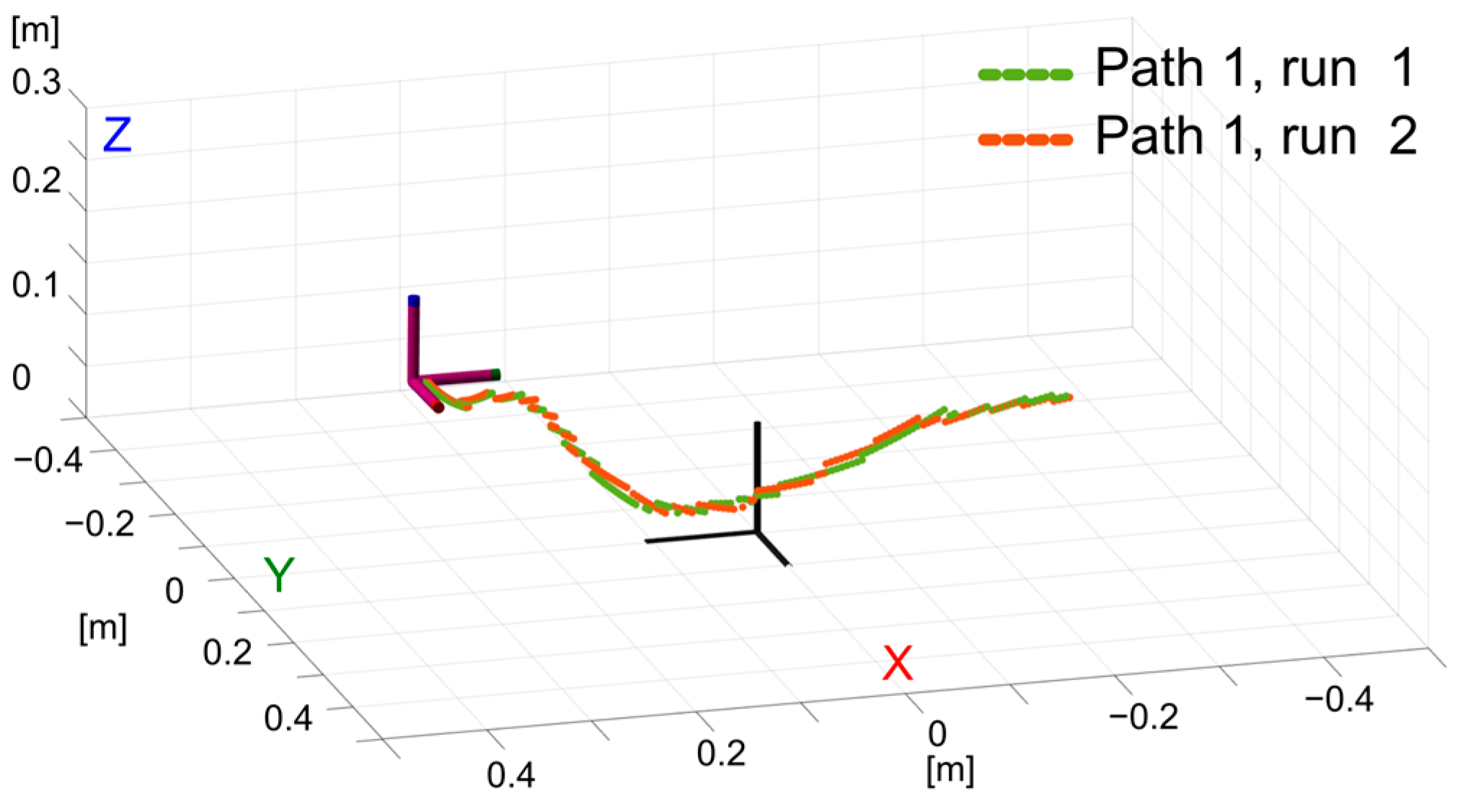
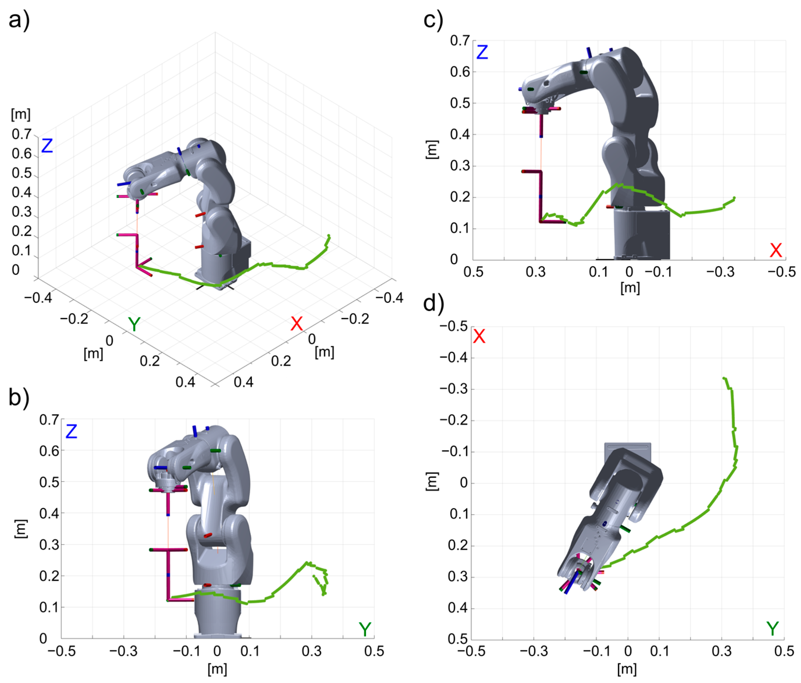
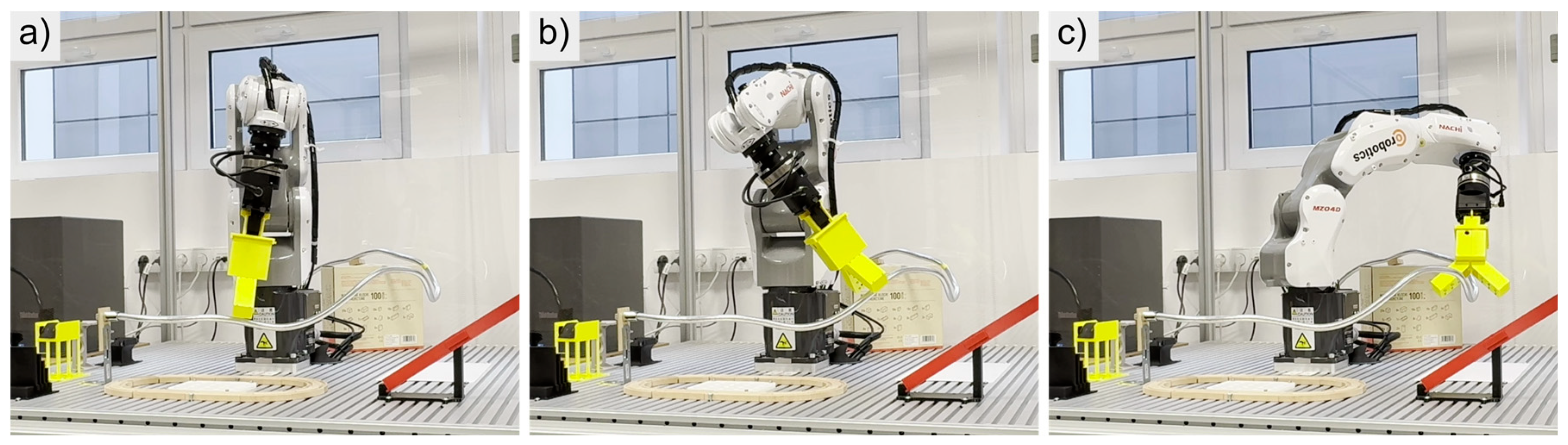
The same path as in the previous run was used and it was also followed with success. Figure 13 presents four views of the detected path and Figure 14—three selected examples of robot positions obtained during path-following. Some differences in the detected path positions compared to run 1 may be noticed, but they are small. Figure 15 presents both runs overlayed, so the differences are easier to notice. The largest difference between detected positions of both paths is 15.2 mm (which is a value similar to the path detection accuracy described in Section 3.1), and the mean difference is 5.2 mm. This test confirms the repeatability of the results obtained using the proposed solution.
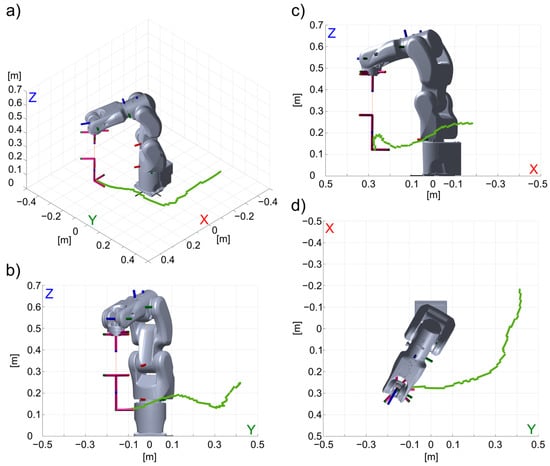
Figure 13.
Path 1, run 2—path (green line) detected by the detection tool (a) isometric view, (b) front view (YZ plane), (c) side view (XZ plane), and (d) top view (YX plane).
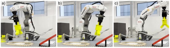
Figure 14.
Path 1, run 2—(a–c) three selected examples of robot positions obtained during path-following; full video available as Supplementary Material [S2].
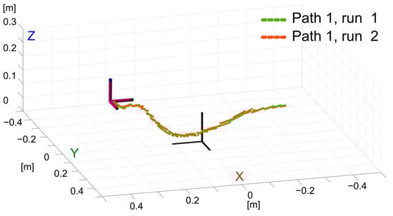
Figure 15.
Path 1, run 1 and 2 overlayed; the robot body is removed for a clearer view.
3.3.3. Path 2, Run 1
In this test, the path had more up and down bends and path arcs had smaller radiuses. This path was also successfully followed. Figure 16 presents four views of the detected path and Figure 17—three selected examples of robot positions obtained during path-following.
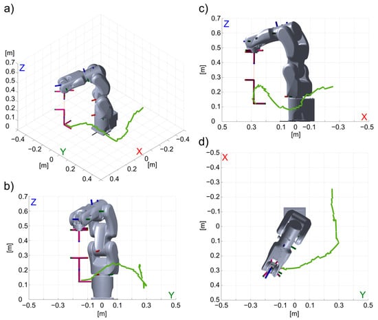
Figure 16.
Path 2, run 1—path (green line) detected by the detection tool (a) isometric view, (b) front view (YZ plane), (c) side view (XZ plane), and (d) top view (YX plane).

Figure 17.
Path 2, run 1—(a–c) three selected examples of robot positions obtained during path-following; full video available as Supplementary Material [S2].
3.3.4. Path 3, Run 1
This path had a longer, almost flat section at the beginning, followed by a high bend section. Additionally, it was placed closer to the robot base in its middle section. At the end of the run, the detection tool slightly collided with the path, but the algorithm was able to correct the tool trajectory and continued properly. This means that the path was, once again, followed with success. Figure 18 presents four views of the detected path and Figure 19—three selected examples of robot positions obtained during path-following.
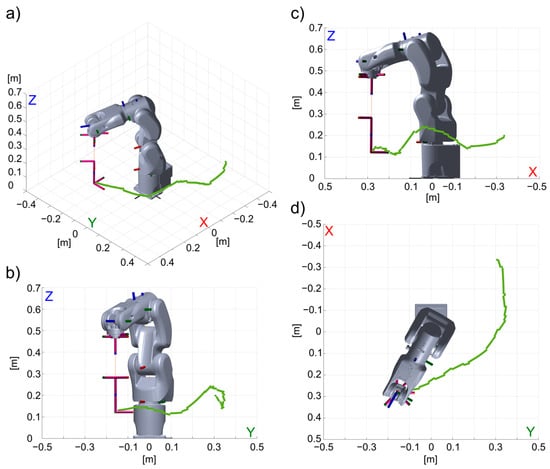
Figure 18.
Path 3, run 1—path (green line) detected by the detection tool (a) isometric view, (b) front view (YZ plane), (c) side view (XZ plane), and (d) top view (YX plane).
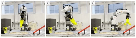
Figure 19.
Path 3, run 1—(a–c) three selected examples of robot positions obtained during path-following; full video available as Supplementary Material [S2].
3.3.5. Path 4, Run 1
This path was shorter, but it differed from the others by being bent in the “outbound” direction (i.e., away from the robot) and then going “up”. In this case, the boundary in the X+ axis was changed to 850 mm, as it was necessary to slightly cross the standard limits of the robot safety cell. The cell doors were open, so there was no collision with the cell during the run. Figure 20 presents four views of the detected path and Figure 21—three selected examples of robot positions obtained during path-following.
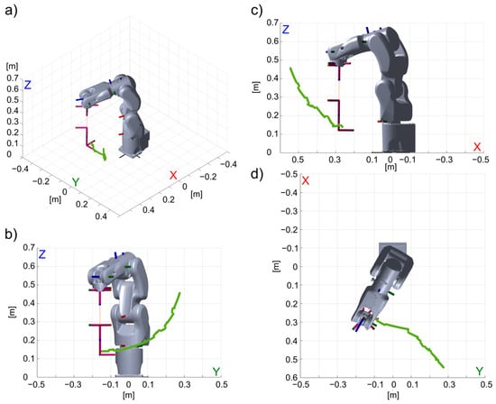
Figure 20.
Path 4, run 1—path (green line) detected by the detection tool (a) isometric view, (b) front view (YZ plane), (c) side view (XZ plane), and (d) top view (YX plane).
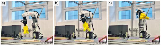
Figure 21.
Path 4, run 1—(a–c) three selected examples of robot positions obtained during path-following; full video available as Supplementary Material [S2].
4. Discussion
The proposed algorithm, despite the simplicity of the measurement tools used and despite being based on the simple, classically inspired line-follower concept, turned out to be effective in following the path defined in a 3D space. Its capabilities and practical effectiveness, however, are limited by the capabilities of the robot itself and the inverse kinematics solver. In particular, these are the issues associated with avoiding the robot’s singular positions when tracing the path, the physical limitations of the robot’s kinematics resulting from its construction, and the size of the working area, limitations of robot movements resulting from, for example, the wiring of the equipment installed on the robot and the physical dimensions of the detection tool and the path itself. During the tests, if the path-following run had to be interrupted (i.e., halted), in most cases it was caused by the inability of the IK solver to find the proper solution due to the robot’s limited workspace or because the expected position was simply impossible to reach for the robot due to its kinematic constraints. This means that the limits of the proposed solution do not lie in the path-following algorithm itself but rather in the limits of the employed robot.
During the experiments, the robot moves were performed with a limited, safe speed of 50 mm/s. Higher speeds may be applied, but when choosing them the step calculation time must be taken into consideration. A limitation might lie in the time needed for the calculation of the next position by the IK solver. During the presented tests, this was usually calculated in a short time (0.25 s on average), but in some difficult to reach positions it took a couple of seconds for the solver to provide a solution. The algorithm was run on a laptop computer with an Intel i5-1340p processor and 16 GB RAM. Another limitation may be caused by the time needed for reading the detection sensors’ state and by the time needed for communication with the robot. During tests, one complete step (starting from the call to read sensor data up to executing and completing the move to the new position) was usually performed in approximately 1.7 s.
The algorithm should work properly when applied with almost no modifications on any articulated robot. Only the robot kinematics description and constraints for the IK solver must be updated to match a different robot. The application of the proposed solution should also be possible for mobile robots, but it would not be as straightforward as in the case of industrial robots and some elements would have to be adapted first. This is one possible goal for further algorithm development and research. Additionally, in the current form the algorithm does not include procedures for processing path splits or intersections, which may be a drawback. However, as each step is calculated based on local detection results only, the path as a whole (i.e., globally) does not have to be predetermined as it is detected step by step. This means that the path may change its shape during path-following. The only limitation is that the path cannot change too much in a close vicinity of the detection tool because in this case the path may leave the detection field. On the other hand, even if the path moves inside the detection field, this would be treated by the algorithm as a path bend, and it will adapt to the new path position.
The ability of the algorithm to follow a sharp path bend depends on many factors. First of all, the physical dimensions of the path and the detection tool limit the tool rotation in subsequent steps. Secondly, during calculations of tool rotation, rotation reduction is applied so the tool cannot be rotated too much. Without reduction, the tool may be extensively rotated in every move when the path is detected in different detection points in two subsequent steps. Reduction decreases this effect. Vector reduction values (a and b in (17)) are adjustable, and their values should therefore be the result of a compromise. Stronger reduction will limit the ability to follow path bends with small arcs but, on the other hand, will reduce the “waving” movement of the tool around the path. This will result in an overall smoother path-following. Additionally, path width (i.e., diameter), detection tool dimensions, sensor spacing and characteristics (ex. cone-shaped detection field), etc., also influence the ability to follow sharp path bends. During the tests, the smallest arc of bend was around 10 cm.
During the experiments, it appeared that sometimes, especially when the tool was moving away from the path, the path was lost and the algorithm was not able to locate it. When the tool was moving towards the path, such a problem almost never occurred. To prevent losing the path, more sensors should be used, and they should be placed more densely. Another solution may be to return to the last successful path detection position if the path is not detected for a given number of steps, and then to restart the moves in a slightly modified direction.
The ToF sensors that were used in the detection tool, as well as Bluetooth communication, proved to be very reliable. In practice, the only malfunctions were caused by the low energy level of the battery powering the tool. In such situations, communication was lost and the path-following procedure was aborted as the battery had to be replaced.
5. Conclusions
Thanks to the result of the presented research, it can be concluded that despite the use of only six low-cost ToF sensors (the price for one sensor breakout module with the sensor and integrated supporting electronics is approximately EUR 11, while one sensor itself costs approximately EUR 2), the low-cost microcontroller and Bluetooth (approximately EUR 15 for the MCU development board and EUR 12 for the Bluetooth module), and standard laptop computer, it was possible to meet the expected goals. This was achieved using simple technical tools and a simple algorithm, without the need for applying a complex method like, for example, AI algorithms, which need long-lasting and high computing power and time-consuming training.
The presented solution is easily scalable. An improvement may be sought by increasing the number of sensors, e.g., to 10 instead of 6. This would improve the number of detection points, increase path detection accuracy, and reduce the occurrence of situations in which the algorithm loses the path or sharp bends in the path occur. The other proposal is to use LiDAR sensors (instead of ToF sensors), which should reduce the size of the detection tool and allow the reading of the position of the path to be much more accurate, not only at the intersections points of the detection zones of ToF sensors.
The presented algorithm together with its implementation (including hardware elements) has a centimetre-level path-following accuracy. It is limited mostly by the detection tool spatial resolution. At the current stage of elaboration, the main goal of this research was to develop the methodology and test it in practice. Further development, as mentioned above, will be directed towards enhancing the path detection accuracy.
When comparing the results to other solutions, it is worth noting that path detection and path-following methods for 2D paths, especially those based on vision systems supported by lasers and AI data processing, achieve even submillimetre-level accuracy. The methods used for 3D navigation and positioning or object and obstacle recognition, used, for example, for UAV or autonomous car control, have various accuracies, starting from metres down to millimetres depending on what is needed for the particular application. The most accurate methods used for object localization in a 3D space are precise structured light scanners. Commercially available scanners may achieve very high, micrometre-level accuracies, but are very expensive and need high computational power for data processing. In this context, the method proposed in this paper may appear inferior, but it is always a trade-off between the desired accuracy and system costs, including hardware and software. Thus, the described solution, even though it cannot match the extremally high accuracies of some of the most advanced solutions, may find applications, especially after detection resolution and accuracy are increased, which is possible within limited costs.
Potential applications of the proposed path-following method are tasks performed in the robot’s workspace that require moving along a previously unknown but physically defined path, for example, contactless scanning or monitoring of various long, narrow objects. After extending the method to mobile robots, specifically aerial or underwater, the proposed idea could be implemented in the tasks of monitoring power lines, pipelines, ropes, or chains, hanging in the air or placed underwater, especially if exact positioning or minimising the path-following error are not of the greatest importance, or the costs need to be kept to a minimum. After increasing path detection accuracy, this approach could also be applied, for example, in some less accuracy-demanding welding, glueing, or 3D printing jobs. The method could also be used as a supplementary add-on to other methods, for example, those relying on vision systems, especially in adverse environments or conditions such as underwater operations, dark areas, or in severe weather conditions.
Supplementary Materials
The supporting information for this paper are available as Open Data. Link S1: Control software and experimental data. 2024. https://doi.org/10.34808/qtp2-7s79; Link S2: Video data set. 2024. https://doi.org/10.34808/92gd-2y47.
Author Contributions
Conceptualization, M.A.G.; methodology, T.F.W., I.D.O. and M.A.G.; validation, M.A.G.; software, T.F.W., I.D.O. and M.A.G.; investigation, T.F.W. and I.D.O.; data curation, T.F.W. and I.D.O.; writing—original draft preparation, T.F.W., I.D.O. and M.A.G.; writing—review and editing, T.F.W., I.D.O. and M.A.G.; visualisation, T.F.W., I.D.O. and M.A.G.; supervision, M.A.G. All authors have read and agreed to the published version of the manuscript.
Funding
This research received no external funding.
Institutional Review Board Statement
Not applicable.
Informed Consent Statement
Not applicable.
Data Availability Statement
The data presented in this study are available in the Supplementary Materials—see [S1,S2].
Acknowledgments
The Nachi MZ04 robot used for experimental investigation was acquired thanks to the internal Gdansk-Tech grant: IDUB CoreEduFacilities 14/2021/EDU—MecHaRo-Lab project.
Conflicts of Interest
The authors declare no conflicts of interest.
References
- Marashian, A.; Razminia, A. Mobile robot’s path-planning and path-tracking in static and dynamic environments: Dynamic programming approach. Robot. Auton. Syst. 2024, 172, 104592. [Google Scholar] [CrossRef]
- Namgung, H. Local Route Planning for Collision Avoidance of Maritime Autonomous Surface Ships in Compliance with COLREGs Rules. Sustainability 2022, 14, 198. [Google Scholar] [CrossRef]
- Debnath, D.; Vanegas, F.; Sandino, J.; Hawary, A.F.; Gonzalez, F. A Review of UAV Path-Planning Algorithms and Obstacle Avoidance Methods for Remote Sensing Applications. Remote Sens. 2024, 16, 4019. [Google Scholar] [CrossRef]
- Ou, X.; You, Z.; He, X. Local Path Planner for Mobile Robot Considering Future Positions of Obstacles. Processes 2024, 12, 984. [Google Scholar] [CrossRef]
- Liu, L.; Wang, X.; Yang, X.; Liu, H.; Li, J.; Wang, P. Path planning techniques for mobile robots: Review and prospect. Expert Syst. Appl. 2023, 227, 120254. [Google Scholar] [CrossRef]
- Tan, C.S.; Mohd-Mokhtar, R.; Arshad, M.R. A Comprehensive Review of Coverage Path Planning in Robotics Using Classical and Heuristic Algorithms. IEEE Access 2021, 9, 119310–119342. [Google Scholar] [CrossRef]
- Thompson, N.; Greenewald, K.; Lee, K.; Manso, G.F. The Computational Limits of Deep Learning. In Proceedings of the Ninth Computing within Limits 2023, Virtual, 14–15 June 2023. [Google Scholar] [CrossRef]
- Youn, W.; Ko, H.; Choi, H.; Choi, I.; Baek, J.-H.; Myung, H. Collision-free Autonomous Navigation of A Small UAV Using Low-cost Sensors in GPS-denied Environments. Int. J. Control Autom. Syst. 2021, 19, 953–968. [Google Scholar] [CrossRef]
- Mekathlon—International Line Follower Robot Competition. Available online: https://www.mekathlon.com/fastest-line-follower (accessed on 18 December 2024).
- Robotex International. Available online: https://robotex.international/line-following/ (accessed on 18 December 2024).
- Minaya, C.; Rosero, R.; Zambrano, M.; Catota, P. Application of Multilayer Neural Networks for Controlling a Line-Following Robot in Robotic Competitions. J. Autom. Mob. Robot. Intell. Syst. 2024, 18, 35–42. [Google Scholar] [CrossRef]
- Magnum Automation Inc. AGV/AGC Assembly Line. Available online: https://www.magnum-inc.com/systems/agvs-agcs/agc-assembly-line/ (accessed on 18 December 2024).
- Mohammed, M.S.; Abduljabar, A.M.; Faisal, M.M.; Mahmmod, B.M.; Abdulhussain, S.H.; Khan, W.; Liatsis, P.; Hussain, A. Low-cost autonomous car level 2: Design and implementation for conventional vehicles. Results Eng. 2023, 17, 100969. [Google Scholar] [CrossRef]
- Zakaria, N.J.; Shapiai, M.I.; Ghani, R.A.; Yassin MN, M.; Ibrahim, M.Z.; Wahid, N. Lane Detection in Autonomous Vehicles: A Systematic Review. IEEE Access 2023, 11, 3729–3765. [Google Scholar] [CrossRef]
- Anand, M.; Kalaisevi, P.; Arun Kumar, S.; Nithyavathy, N. Design and Development of Automated Guided Vehicle with Line Follower Concept using IR. In Proceedings of the 2023 Fifth International Conference on Electrical, Computer and Communication Technologies (ICECCT), Erode, India, 22–24 February 2023; pp. 1–11. [Google Scholar] [CrossRef]
- Jang, J.-Y.; Yoon, S.-J.; Lin, C.-H. Automated Guided Vehicle (AGV) Driving System Using Vision Sensor and Color Code. Electronics 2023, 12, 1415. [Google Scholar] [CrossRef]
- Bach, S.; Yi, S. An Efficient Approach for Line-Following Automated Guided Vehicles Based on Fuzzy Inference Mechanism. J. Robot. Control 2022, 3, 395–401. [Google Scholar] [CrossRef]
- Engin, M.; Engin, D. Path Planning of Line Follower Robot. In Proceedings of the 5th European DSP Education and Research Conference (EDERC), Amsterdam, The Netherlands, 13–14 September 2012; pp. 1–5. [Google Scholar] [CrossRef]
- Mahaleh, M.; Mirroshandel, S. Real-time application of swarm and evolutionary algorithms for line follower automated guided vehicles: A comprehensive study. Evol. Intell. 2022, 15, 119–140. [Google Scholar] [CrossRef]
- Moshayedi, A.J.; Zanjani, S.M.; Xu, D.; Chen, X.; Wang, G.; Yang, S. Fusion based AGV Robot Navigation Solution Comparative Analysis and Vrep Simulation. In Proceedings of the 8th Iranian Conference on Signal Processing and Intelligent Systems (ICSPIS), Behshahr, Iran, 28–29 December 2022; pp. 1–11. [Google Scholar] [CrossRef]
- Liu, G.; Sun, W.; Xie, W.; Xu, Y. Learning visual path–following skills for industrial robot using deep reinforcement learning. Int. J. Adv. Manuf. Technol. 2022, 122, 1099–1111. [Google Scholar] [CrossRef]
- Manorathna, R.P.; Phairatt, P.; Ogun, P.; Widjanarko, T.; Chamberlain, M.; Justham, L.; Marimuthu, S.; Jackson, M.R. Feature extraction and tracking of a weld joint for adaptive robotic welding. In Proceedings of the 13th International Conference on Control Automation Robotics & Vision (ICARCV), Singapore, 10–12 December 2014; pp. 1368–1372. [Google Scholar] [CrossRef]
- Mathoworks Minidrone Competition. Available online: https://www.mathworks.com/academia/students/competitions/minidrones.html (accessed on 18 December 2024).
- Basso, M.; Pignaton de Freitas, E. A UAV Guidance System Using Crop Row Detection and Line Follower Algorithms. J. Intell. Robot. Syst. 2020, 97, 605–621. [Google Scholar] [CrossRef]
- da Silva, Y.M.R.; Andrade, F.A.A.; Sousa, L.; de Castro, G.G.R.; Dias, J.T.; Berger, G.; Lima, J.; Pinto, M.F. Computer Vision Based Path Following for Autonomous Unmanned Aerial Systems in Unburied Pipeline Onshore Inspection. Drones 2022, 6, 410. [Google Scholar] [CrossRef]
- Schofield, O.B.; Iversen, N.; Ebeid, E. Autonomous power line detection and tracking system using UAVs. Microprocess. Microsyst. 2022, 94, 104609. [Google Scholar] [CrossRef]
- Pussente, G.A.N.; de Aguiar, E.P.; Marcato, A.L.M.; Pinto, M.F. UAV Power Line Tracking Control Based on a Type-2 Fuzzy-PID Approach. Robotics 2023, 12, 60. [Google Scholar] [CrossRef]
- Xiang, X.; Yu, C.; Niu, Z.; Zhang, Q. Subsea Cable Tracking by Autonomous Underwater Vehicle with Magnetic Sensing Guidance. Sensors 2016, 16, 1335. [Google Scholar] [CrossRef]
- Gerigk, M.K.; Gerigk, M. Application of unmanned USV surface and AUV underwater maritime platforms for the monitoring of offshore structures at sea. Sci. J. Marit. Univ. Szczec. 2023, 76, 89–100. [Google Scholar]
- Ziebinski, A.; Mrozek, D.; Cupek, R.; Grzechca, D.; Fojcik, M.; Drewniak, M.; Kyrkjebø, E.; Lin, J.C.-W.; Øvsthus, K.; Biernacki, P. Challenges Associated with Sensors and Data Fusion for AGV-Driven Smart Manufacturing. In Computational Science—ICCS 2021; Paszynski, M., Kranzlmüller, D., Krzhizhanovskaya, V.V., Dongarra, J.J., Sloot, P.M., Eds.; Lecture Notes in Computer Science; Springer: Cham, Switzerland, 2021; Volume 12745. [Google Scholar] [CrossRef]
- Ghambari, S.; Golabi, M.; Jourdan, L.; Lepagnot, J.; Idoumghar, L. UAV path planning techniques: A survey. RAIRO-Oper. Res. 2024, 58, 2951–2989. [Google Scholar] [CrossRef]
- ul Husnain, A.; Mokhtar, N.; Mohamed Shah, N.; Dahari, M.; Iwahashi, M. A Systematic Literature Review (SLR) on Autonomous Path Planning of Unmanned Aerial Vehicles. Drones 2023, 7, 118. [Google Scholar] [CrossRef]
- Meyes, R.; Tercan, H.; Roggendorf, S.; Thiele, T.; Büscher, C.; Obdenbusch, M.; Brecher, C.; Jeschke, S.; Meisen, T. Motion Planning for Industrial Robots using Reinforcement Learning. Procedia CIRP 2017, 63, 107–112. [Google Scholar] [CrossRef]
- Guo, Q.; Yang, Z.; Xu, J.; Jiang, Y.; Wang, W.; Liu, Z.; Zhao, W.; Sun, Y. Progress, challenges and trends on vision sensing technologies in automatic/intelligent robotic welding: State-of-the-art review. Robot. Comput.-Integr. Manuf. 2024, 89, 102767. [Google Scholar] [CrossRef]
- Maldonado-Ramirez, A.; Rios-Cabrera, R.; Lopez-Juarez, I. A visual path-following learning approach for industrial robots using DRL. Robot. Comput.-Integr. Manuf. 2021, 71, 102130. [Google Scholar] [CrossRef]
- Slabaugh, G.G. Computing Euler Angles from a Rotation Matrix; Technical Report; University of London: London, UK, 1999; pp. 39–63. [Google Scholar]
- Nachi Fujikoshi Corp. Manipulator Instruction Manual, MMZEN-288-013; Nachi Fujikoshi Corp: Toyama City, Japan, 2021. [Google Scholar]
- ST Microelectronics. VL6180X Proximity and Ambient Light Sensing (ALS) Module Datasheet, 2016. Available online: https://www.st.com/resource/en/datasheet/vl6180x.pdf (accessed on 13 February 2025).
- Nachi Fujikoshi Corp. CFDS Controller Instruction Manual User Task, CFDs-EN-123-001A; Nachi Fujikoshi Corp: Toyama City, Japan, 2021. [Google Scholar]
- Mathworks, GeneralizedInverseKinematrics Object Documentation. Available online: https://www.mathworks.com/help/robotics/ref/generalizedinversekinematics-system-object.html (accessed on 7 January 2025).
- Press, W.H.; Teukolsky, S.A.; Vetterling, W.T.; Flannery, B.P. Numerical Recipes in C, The Art of Scientific Computing, 2nd ed.; Cambridge University Press: Cambridge, UK, 1992; ISBN 0-521-43108-5. [Google Scholar]
- Liwiński, K.; Budzisz, D. Testing the Capabilities of the Nachi MZ04 Robot in Terms of Performing Tasks with External Control. B.Sc. (Eng.) Thesis, Gdańsk University of Technology, Gdańsk, Poland, 2024. (In Polish). [Google Scholar]


Disclaimer/Publisher’s Note: The statements, opinions and data contained in all publications are solely those of the individual author(s) and contributor(s) and not of MDPI and/or the editor(s). MDPI and/or the editor(s) disclaim responsibility for any injury to people or property resulting from any ideas, methods, instructions or products referred to in the content. |
© 2025 by the authors. Licensee MDPI, Basel, Switzerland. This article is an open access article distributed under the terms and conditions of the Creative Commons Attribution (CC BY) license (https://creativecommons.org/licenses/by/4.0/).