Abstract
Resistance is a key index of a ship’s hydrodynamic performance, and studying the design of the bulbous bow is an important method to reduce ship resistance. Based on the ship resistance sample data obtained from computational fluid dynamics (CFD) simulation, this study uses a machine learning method to realize the fast prediction of ship resistance corresponding to different bulbous bows. To solve the problem of insufficient accuracy in the single surrogate model, this study proposes a CBR surrogate model that integrates convolutional neural networks with backpropagation and radial basis function models. The coordinates of the control points of the NURBS surface at the bulbous bow are taken as the design variables. Then, a convergence factor is introduced to balance the global and local search abilities of the whale algorithm to improve the convergence speed. The sample space is then iteratively searched using the improved whale algorithm. The results show that the mean absolute error and root mean square error of the CBR model are better than those of the BP and RBF models. The accuracy of the model prediction is significantly improved. The optimized bulbous bow design minimizes the ship resistance, which is reduced by 4.95% compared with the initial ship model. This study provides a reliable and efficient machine learning method for ship resistance prediction.
1. Introduction
A low-resistance hull structure plays a crucial role in improving the performance of a ship [1], and the bulbous bow is widely used in the ship design process to reduce the ship’s wave resistance. In the early 20th century, Taylor conducted experiments on a ship with a bulbous bow, demonstrating the impact of the bow on the ship’s performance. He then installed bulbous bows on U.S. Navy battleships for the first time. Wigley [2] investigated the linearized wave resistance theory and successfully resolved the wave cancellation problem, thus verifying Taylor’s work from a theoretical perspective. Maruo [3] employed the theory of minimum wave resistance for bulbous bow vessels and utilized a variational approach to derive the best cross-sectional area curve and the ideal dimensions of the bulbous bow. This study indicated that vessels featuring a cylindrical bulbous bow were not invariably optimal at elevated design speeds. A ship’s cross-sectional area and the configuration of the bulbous bow are closely related to the resistance to ascending waves. Baniela [4] conducted a study on the first tugboat with a bulbous bow, produced in a shipyard in Spain in 2005. The results indicated that the bulbous bow is beneficial for the escorting of tugboats. It can mitigate resistance by producing a wave that complements its own geometry. However, the bulbous bow may be detrimental because of the dominance of viscous resistance at low speeds. In a recent review, El-Ela [5] analyzed the impact of a bulbous bow on the hydrodynamic performance of a ship, noting that the effective power necessary for the motion of the ship correlates with the speed and resistance. The presence of the bulbous bow reduces the effective power, and its performance is influenced by the shape and the Froude number (). The paper indicates that the beneficial range is between 0.238 and 0.563, thus designing an appropriate bulbous bow is key to reducing the ship’s resistance.
Early ship resistance prediction mainly relied on empirical formulas, such as the Holtrop formula and the ITTC formula. These formulas typically estimate resistance based on geometric parameters (such as aspect ratio and draft depth) and factors like speed. However, as technology has advanced, modeling tests can now simulate the complex hydrodynamic effects of actual currents. A ship hull using a downsized model can be used in a pool for the towing test to predict the resistance. This method reflects the change in resistance under different ship types and speeds with a higher degree of accuracy. It has the potential to more accurately represent the evolution of resistance as a result of varying ship types and speeds and to progressively replace the empirical formula. Lee [6] conducted towing tests on three kinds of hulls with different bows and proved that the effect of the wave amplitude on the added resistance was not negligible. So the geometry of the hull needs to be taken into account in the resistance calculation. The advent of the CFD method in the early 20th century offers a novel approach for contemporary ship resistance prediction. The CFD approach utilizes computational fluid dynamics numerical analysis technology to determine ship resistance more accurately by solving the Navier–Stokes equations. Luo and Lan [7] integrated CAESES with CFD to establish a completely automated framework for parametric modeling, hydrodynamic analysis, design assessment, and shape alteration. Recent scholarly studies on ship resistance utilizing computational fluid dynamics have predominantly focused on the following three components: ship modeling, CFD simulation, and optimization design. Le et al. [8] designed a novel bulbous bow and demonstrated through CFD methods that it influences both the pressure distribution on the ship’s free surface and the wave pattern under full load conditions. Díaz Ojeda [9] provided a reverse design methodology to examine the hydrodynamic performance resulting from the removal of the bulbous bow in a fishing vessel, offering a novel perspective for ship design concepts.
Nonetheless, as the current ship simulation calculations advance, efficiency concerns are increasingly becoming a factor. Design optimization utilizing the CFD method frequently necessitates numerous iterative calculations, potentially resulting in significant expenses for intricate flow issues. Jiang [10] applied NURBS integral formulas to hull parameters, simplifying the computation of the cross-sectional area curve, design waterline, and transverse sections to meet engineering requirements. Yang et al. [11] noted that achieving high accuracy with CFD approaches requires substantial computational resources, posing a paradoxical challenge. CFD relies on commercial simulation software, requiring the purchase of usage rights, which incurs costs.
Machine learning has been extensively employed in the field of ship engineering and has undergone rapid development in recent years. Many researchers have employed surrogate models to approximate CFD simulations in response to these issues. The optimal longitudinal inclination of a container ship was determined by Tu et al. [12] through a comparison of various models. Subsequently, they proposed a method that can rapidly predict the optimal longitudinal inclination of an arbitrary container ship. The random forest prediction model was selected as the optimal prediction model. Nazemian [13] utilized regression tree (RT), support vector machine (SVM), and artificial neural network (ANN) regression models to develop a predictor of calm water resistance for catamaran hull forms. The ship performance was optimized for various types, including resistance-based dimension and hull coefficient optimization, as well as structural weight and battery performance improvements. Based on their research, the model’s performance may vary significantly across different ship data. This introduces additional workload, and a universal model with more features is urgently needed. Tran et al. [14] optimized planing hulls at high speeds by focusing on lift and complex hydrodynamic interactions, identifying the optimal hull shape to minimize resistance using a Kriging surrogate model and the Nelder–Mead algorithm. Zhang [15] introduced a deep trust network algorithm for estimating the total resistance of various hull modifications. This algorithm was compared with traditional models, namely ELMAN and RBF neural networks, revealing that the deep trust network algorithm effectively achieves the optimal solution for minimizing the total resistance across different speeds. The aforementioned article illustrates the advantages of surrogate models in ship design; however, the impact of the localized hull design on resistance remains significant owing to the multi-layered structure of the hull. Liu et al. [16] conducted an optimal design for the calm water resistance of a high-speed catamaran hull, employing a Kriging model to create a new bulbous bow and utilizing a genetic algorithm to identify the two best vessels with minimal wave resistance. Yongxing et al. [17] employed the dimensions of the bulbous bow, specifically its length and width, along with the angle relative to the baseline, as optimization variables. They used a non-dominated sorting genetic algorithm (NSGA)-II within the CFD solver STAR-CCM+ to identify the optimal ship type. This approach mitigated the errors associated with indirect model construction; however, the complexity and time-consuming nature of the CFD coupled with additional algorithmic iterations may exacerbate this situation.
The main works and contributions of this study are as follows: (1) A parameterized modeling process for ship hull spherical bow shapes has been established based on NURBS surface construction. Using the DTMB5415 ship model as an example, the free-form deformation method was employed to modify the shape of the spherical bow. Furthermore, computational fluid dynamics (CFD) simulations were conducted to collect data on ship resistance. (2) To address the issue of long computational times associated with CFD simulations, a rapid prediction model for ship resistance based on CFD simulation data was developed. A hybrid surrogate model construction framework was proposed to improve model accuracy based on prediction errors. (3) An improved whale optimization algorithm was implemented to perform optimization of the spherical bow shape based on the surrogate model, enabling the identification of the shape that minimizes ship hull resistance.
The structural framework of this paper is as follows: Section 2 presents the materials and fundamental methods used. Section 3 discusses the experimental results and provides a validation of these results. Section 4 engages in a discussion of the experimental findings, analyzing the contributions and limitations of the research, and suggests directions for future work. Finally, Section 5 summarizes the work of this paper.
2. Materials and Methods
2.1. Ship Model Design
The precision of the hull model is essential for software simulation and forecasting the hydrodynamic performance of a ship. Parametric modeling of the hull typically involves three steps: selecting characteristic parameters, designing longitudinal and transverse characteristic curves, and generating the hull surface. The components of the hull profile encompass the cross-sectional curve, design waterline, hull profile curve, bow profile curve, and stern profile curve. Typically, these profiles are integrated into linear segments, quadratic curves, and arbitrary curves.
Non-uniform rational B-spline (NURBS) curves are widely used in ship hull modeling, allowing shape manipulation through control points and weights for smooth surface transitions [18]. A NURBS curve C of order q can be characterized by a rational polynomial vector function, represented by the following expression:
where represents the weight factor for constructing the control polygon, denotes the control point for the formation of the control polygon, and is a q-times B-spline function defined on a non-periodic node vector U.
NURBS surfaces are characterized by an additional parameter in one direction compared to NURBS curves. A NURBS surface S defined q times in the u direction and t times in the v direction can be expressed as a two-parameter rational polynomial vector function, as follows:
where is the weight factor, is the control point, and and are q-times and t-times B-spline functions defined on the non-periodic node vectors U and V.
2.2. Ship Dimensions
The DTMB5415 is a destroyer developed in the U.S. Navy and is among the standard ship models endorsed by the ITTC. Table 1 presents the primary characteristics of the DTMB5415 ship model, with the hull parametrically modeled using NURBS curves and surfaces. This serves as the foundational ship model for optimizing the design of the bulbous bow section to achieve minimal overall resistance. In the next CFD simulation, the scaling ratio was established at 1:25 to enhance the computational efficiency. Figure 1 illustrates the ship’s appearance in the Rhino 7.

Table 1.
The DTMB5415 boat model’s main parameters.

Figure 1.
DTMB5415 hull model.
2.3. Free-Form Deformation Method
The free-form deformation (FFD) method in ship structure modeling allows for the visualization of shape alterations on a computer, thereby enhancing control over the hull configuration. Proposed by Sederberg and Parry [19], it has become a key tool in modern ship design, after years of development. This approach does not directly alter the object. Instead, it incorporates the object into the spatial geometry and achieves deformation by adjusting the moving geometry control points. A local coordinate system is formed on the geometry, designating as the coordinate origin, with any grid point on the geometry expressible as follows:
where is the coordinate value of any grid point in the local coordinate system.
Upon establishment of the local coordinate system, the mapping relationship between the control points of the bulbous bow surface and the control points of the geometry are defined using polynomial basis functions:
where , , are polynomial basis functions along the directions ; denotes the coordinate value of the control point; and denote the number of control points for the three polynomial basis functions.
In the choice of polynomial basis functions, the NURBS basis function greatly increases the flexibility of the deformation by introducing a weighting factor that defines the P-times NURBS basis function N in the direction:
where is the weight coefficient along the direction, and is the B-spline basis function along the direction.
Substituting the other NURBS basis functions into the above definition, the mapping relation becomes as follows:
2.4. Bulbous Bow Deformation
This study employed the FFD method to achieve deformation of the bulbous bow section of the DTMB5415 ship model by manipulating the control points of its NURBS surface. Initially, the ship model was created using Rhino modeling software, and the NURBS surface control points were extracted using the Grasshopper plug-in. The control points of the bulbous bow were selected for modification, and appropriate constraints were established based on actual conditions. The parameter samples were generated based on these constraints to manipulate the NURBS control points, which were then regenerated to finalize the bulbous bow deformation. The software generates a NURBS surface to facilitate the deformation of the bulbous bow, and the resultant deformed hull is recorded in IGES format, as illustrated in Figure 2.
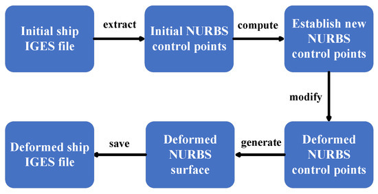
Figure 2.
Flow chart of the parametric geometric deformation of a bulbous bow.
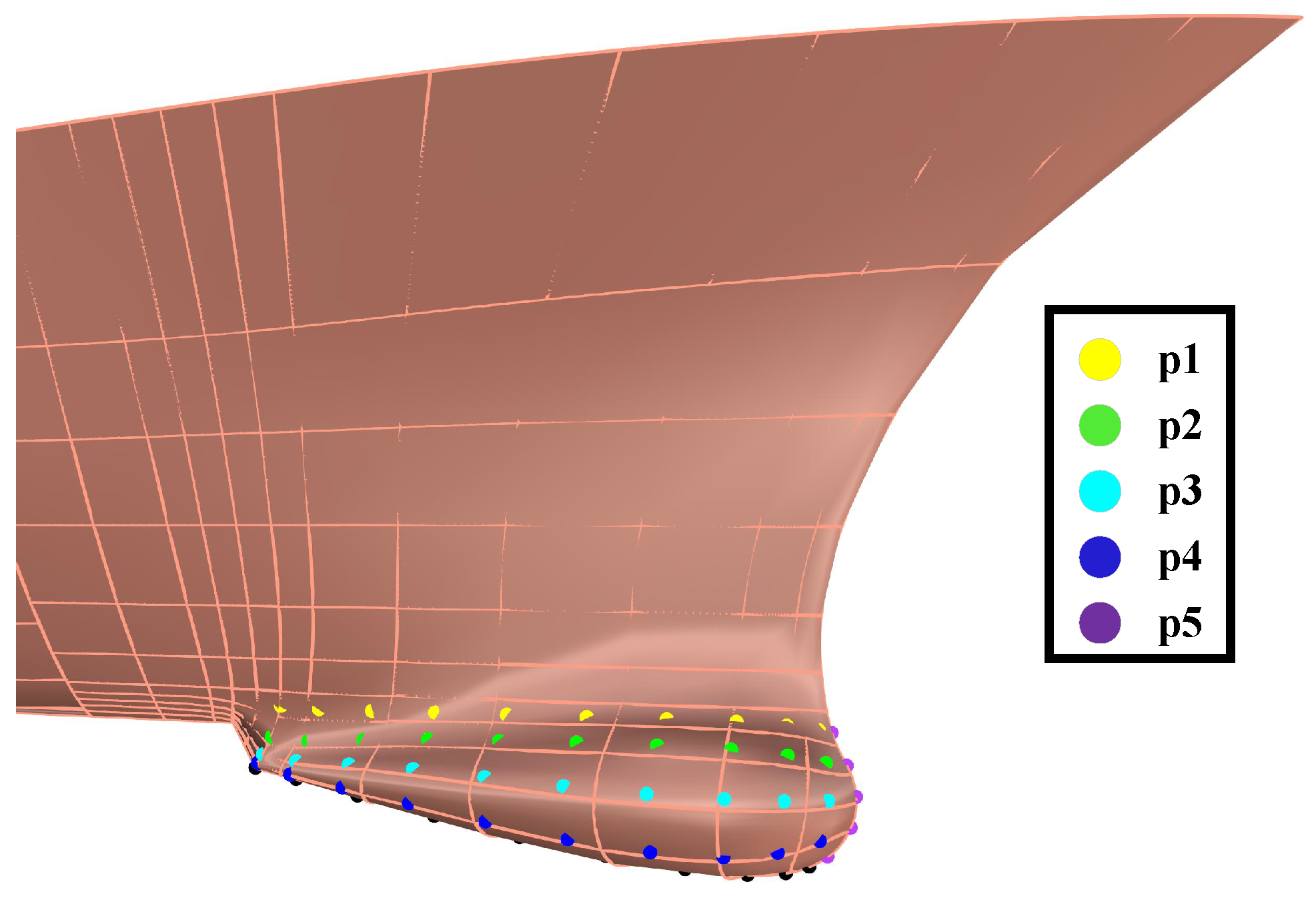
During the software extraction process, numerous control points are typically acquired, and the resultant surface may exhibit irregularities during the subsequent manipulation of these control points. Therefore, to ensure that the surface of the deformed bulbous bow is smooth and level, the control points must be uniformly distributed with adequate spacing between them. Figure 3 illustrates the selection of control points for the preliminary bulbous bow.
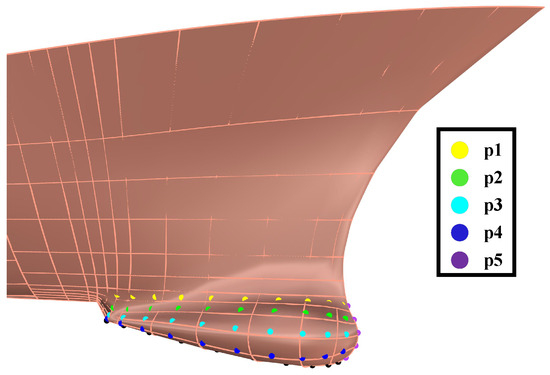
Figure 3.
Distribution of NURBS control points on a bulbous bow.
In the parameter design, as illustrated in Figure 3, we manipulated the control points along the x-axes, y-axes, and z-axes to alter the dimensions of the bulbous bow. The y coordinate of the four sets of control points, designated as , is established as the characteristic parameter for width, whereas the x and z coordinates of serve as the characteristic parameters for the length and height, respectively. To ensure that the configuration of the generated bulbous bow closely resembles the original ship shape, the design minimizes the number of parameters to reduce model complexity. The width feature parameter of the y coordinate utilizes proportional adjustments of the shifted control points. The limitations of the design variables are determined based on actual needs, as shown in Table 2.
Table 2.
Range of values of design variables for a bulbous bow.
Figure 4 shows the process of deforming the bulbous bow. First, the blue NURBS control points on the initial ship bulbous bow are obtained from step a; then, the coordinates of the control points are shifted using FFD to generate the green control points in step b. Finally, the new NURBS surface is generated from step c. Compared with the direct deformation of the bulbous bow by embedding it into a cube, this method can realize more complex shape changes.
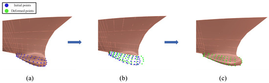
Figure 4.
Process of the deformation of a bulbous bow. (a) extract control points; (b) move control points; (c) generate bulbous bow surface.
2.5. CFD Simulation
In recent years, the computational fluid dynamics (CFD) method has been widely used to simulate the navigation state of hulls under complex environmental conditions. Therefore, this paper realizes the hydrodynamic virtual experiments of the surface hull model based on the CFD core solver, predicts the drag performance and motion attitude under the design speed, and obtains the experimental results of the ship resistance.
In the numerical simulation of the free surface bypassing problem of a surface vessel, the free surface is treated by the level–set method [20]. The hull flow field is computed in the region where the distance function , which avoids the transition problem of the airflow field. In the Level–Set method, the position of the free surface is determined by the value of the numerical function . The distance function satisfies the following equation:
where denotes the distance of any point in the flow field from the free surface.
The flow was simulated using the RANS equation [21], which separates the instantaneous quantities in the turbulent flow into mean and pulsating values. An averaging operation was conducted on the N-S equation to obtain the Reynolds stress term. Additional conditions and relations needed to be sought to obtain the turbulence model to avoid the unsolvability of the RANS equations during the solution process. The SST – turbulence model equations are defined as follows:
Special dissipation rate equations:
where , are the diffusion coefficients for k and ; , are the turbulence generation terms; and , are the turbulence dissipation terms.
In the solution process, the finite difference method [22] is used. The partial derivatives in the partial differential equations are replaced by the difference quotients of the function values at adjacent discrete points, forming a system of algebraic equations. Each node corresponds to an algebraic equation, with the unknowns being the function values at that node and its adjacent nodes. The SIMPLE algorithm [23] is used to handle the pressure–velocity coupling problem, and the pressure field is computed on the grid to solve the momentum equation.
2.6. Error-Based Ensemble Prediction Model
Neural networks can form intricate input–output relationships via multilayer nonlinear transformations, making them appropriate for multivariate nonlinear issues regarding the impact of bulbous bows on ship resistance. Consequently, this study selected the backpropagation (BP) neural network [24] and radial basis function (RBF) neural network [25] as the foundational prediction models. The BP neural network comprises input, hidden, and output layers, with one or more hidden layers, each containing multiple nodes. The interconnections between nodes across layers are represented by weights, which enhance the nonlinear fitting and generalization capabilities. The structure is illustrated in Figure 5, and the mapping relationship is expressed as follows:
where y is the output value of the network, is the activation function, and and b are the weights and biases of the node-to-node connections.
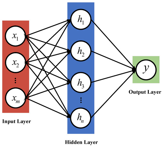
Figure 5.
BP neural network structure diagram.
During the training process, a loss function is formed based on the difference between the output and the expectation. The weights and thresholds are adjusted using the gradient descent method to minimize the loss function.
In contrast to BP networks, the hidden layer of an RBF network consists of a set of radial basis functions with different parameters. The radial basis functions take values dependent on a real-valued function of the distance from the origin: , or the distance to any specified point: . The hidden layer converts input vectors from a low-dimensional space to a high-dimensional hidden space, transforming a previously nonlinear and inseparable scenario into a linear problem, thereby enhancing the learning speed and mitigating the local minimum issue. The mapping relationship of the hidden layer in an RBF network using a Gaussian kernel function as the basis function is defined as follows:
where is the width of the ith Gaussian kernel function, is the center of the ith Gaussian kernel function, and , where is the maximum Euclidean distance between all centers.
The accuracy of surrogate models, as an efficient prediction method for approximating the CFD simulation results, is usually obtained based on the sum of the error averages of the dataset, which is a metric given from the whole. For localized samples in the dataset, the accuracy of one model may not be better than the other, even if there is a significant difference in their error averages. Taking the BP and RBF models as examples, Table 3 lists some of the ship resistance results obtained for a particular training as well as the actual sample values. The calculations show that for the five sample points, the mean error of the BP model is 1.1124 and that of the RBF model is 0.7861. From the data in the table, it can be seen that although the mean error of the RBF model is smaller, the BP prediction is more accurate for the first two sample points. This phenomenon demonstrates the limitation of the accuracy of using a single surrogate model.
Table 3.
Partial training results of the BP and RBF models.
Therefore, this paper proposes a surrogate model based on convolutional neural networks that integrates BP and RBF models, called the CBR agent model. The model can be divided into three modules with the structure shown in Figure 6. The prediction module uses different single surrogate models—the BP neural network and RBF neural network—to train the original samples and input the prediction error of each sample point into the decision module. The decision module uses a convolutional neural network (CNN) [26] to train the original sample inputs along with the acquired errors. It then extracts the spatial features of the sample points to determine the prediction errors of the BP and RBF networks. The function of the selection module is to execute the results of the decision module. For a new sample point input into the CBR model, the selection module selects the model with the lowest error from the prediction module based on the decision result of the decision module.
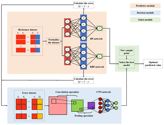
Figure 6.
CBR model structure diagram.
Compared with traditional prediction models, the CBR model improves the judgment of different models for the prediction accuracy of sample points in different spatial regions, integrates multiple single surrogate models, and improves the divisibility of the samples. When faced with complex nonlinear problems and prediction deviations in BP and RBF networks, this model is able to correctly select the network with the smaller deviation. At the same time, it combines the global and local nonlinear mapping capabilities of the BP and RBF networks with the classification ability of CNN, improving the accuracy limitations of a single model.
2.7. Improved Whale Algorithm for Predicting Optimal Resistance
Metaheuristic optimization algorithms perform excellently when dealing with complex nonlinear problems. For the mapping relationship between the spherical bow dimensions and ship resistance constructed by the CBR model, they can obtain the minimum ship resistance and the corresponding spherical bow dimensions. The whale optimization algorithm (WOA) [27], inspired by the hunting behavior of humpback whales, continuously updates the positions of individual whales to identify an optimal solution. This algorithm is distinguished by its minimal number of parameters, ease of implementation, and adaptability. The search process was categorized into three stages:
- (1)
- Enveloping the prey.
Assuming that the position of the best whale individual in space is and that the other individuals move toward it to encircle the prey, the change in the individual’s position X at the next moment can be expressed as follows:
where D is the distance between the individual and the prey, t is the current number of iterations, A and C are computational coefficients, and are random numbers between 0 and 1, and the value of a is determined by the number of iterations, decreasing from 2 to 0 linearly.
- (2)
- Bubble net attack.
Bubble netting, a predatory behavior unique to whales, involves expelling bubbles to deter prey through spiral swimming. It can be represented by the following two mathematical models: contraction encirclement and spiral position update. In contraction encirclement, the process is analogous to the surrounding prey in the model, with the range of parameter A modified from to . In the bubble net assault, the whale selects the contraction encirclement and spiral position update with a chance of 50%, represented as follows:
where p is a random number between 0 and 1, b is a logarithmic spiral shape constant, and l is a random number between −1 and 1.
- (3)
- Search predation.
To ensure the sufficiency of the search and avoid becoming trapped in local optima, the WOA updates the positions based on the relative positions of the whale individuals. Its mathematical model is as follows:
where denotes a randomly selected whale location when .
From the above principle, it can be seen that the whale algorithm calculates the coefficient when the linear parameter a decreases to 1. At this time, the algorithm no longer carries out a stochastic search, which leads to the inability to find the global optimal solution. Therefore, parameter a is improved to a nonlinear convergence factor , which enables the algorithm to adaptively adjust the convergence speed according to the current iteration state. This is conducive to the balance between global exploration and local exploitation, and its updated formula is as follows:
where is the maximum number of iterations. The steps of the improved WOA algorithm are listed in Algorithm 1.
| Algorithm 1 The improved WOA algorithm |
|
3. Results
3.1. Sample Extraction Results and Model Parameter Settings
The quality of the sample set has a significant impact on the results of the model training. Based on the geometric variables of the hull bulbous bow determined in Table 2, this study employed the Latin hypercube sampling (LHS) [28] method to uniformly generate 300 orthogonally distributed sample points in the design space, as shown in Figure 7. To verify the reliability of the LHS scheme, a nearest-neighbor analysis was conducted for all points. Specifically, the distance between each point and its nearest neighbor was calculated, and the mean and variance of all values were determined. These results were then compared with those of a random sampling scheme. The results are shown in Table 4.
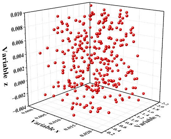
Figure 7.
Latin hypercube sampling points.
Table 4.
Comparison of the mean and variance between each point and its nearest point in two sampling schemes.
Resistance values for the 300 sample ship types were acquired using a CFD solver. The basis prediction model, the BP neural network, utilized logsig and purelin as activation functions, with a hidden layer of 10 neurons. Training was concluded upon achieving a target minimum error of . The RBF neural network established a maximum of 20 neurons, with training concluding once the mean square error objective was achieved at . In the CNN classification model, given that the input samples in this study consisted of one-dimensional sequence data, the convolution kernel size was configured to 2 × 1, the pooling layer size was set to 2 × 1, and the stride was set to 2. The ReLU function was selected as the activation function, the Adam gradient descent technique was used for optimization, and the learning rate was set to 0.001.
3.2. Model Accuracy Evaluation
To evaluate the effectiveness of the CBR model, 300 independent sample points obtained through CFD simulations were used to train three surrogate models: BP, RBF, and CBR. The proportions of training and test sets in the dataset were set to 80% and 20%, respectively, and the test set was an independent sample. The mean absolute error (MAE) and root mean square error (RMSE) were designated as evaluation metrics for the models. Table 5 illustrates the mean and median values of several models based on the sample data, with all measures executed independently 200 times.
Table 5.
Comparison of MAE and RMSE for three models.
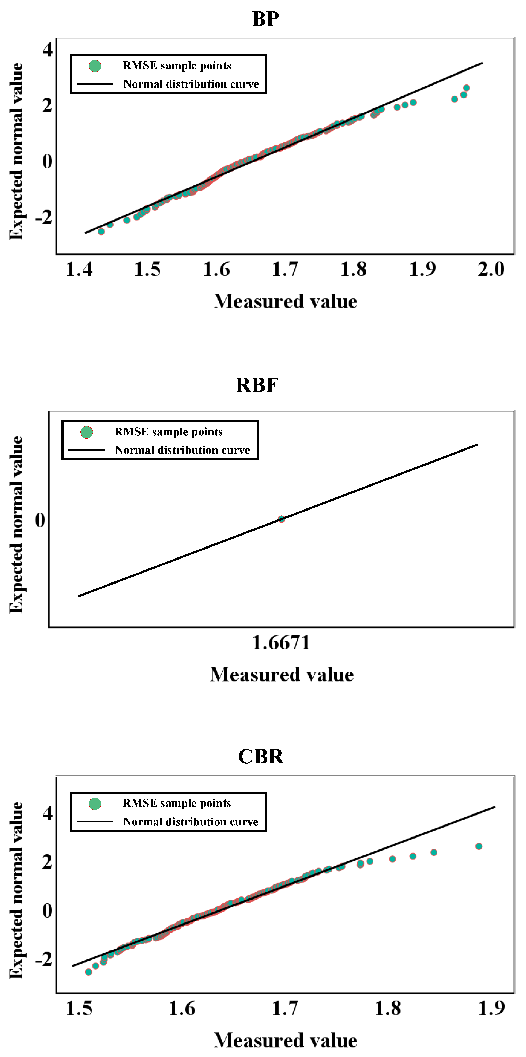
To ascertain whether the model presented in this research has a distinct data distribution compared to the outcomes of other models, the sample data were subjected to significance analysis. Initially, data from 200 independent runs were utilized as samples for the normal distribution test, and the Kolmogorov–Smirnov test (K-S test) was selected based on the sample size. It was assumed that the MAE and RMSE data of the three models followed a normal distribution, thus accepting the null hypothesis when the significance p-value exceeded 0.05. Figure 8 and Figure 9 show the normal Q-Q plots for the three models. The plots demonstrate the distribution of sample data for the MAE and RMSE, with specific values shown in Table 6.
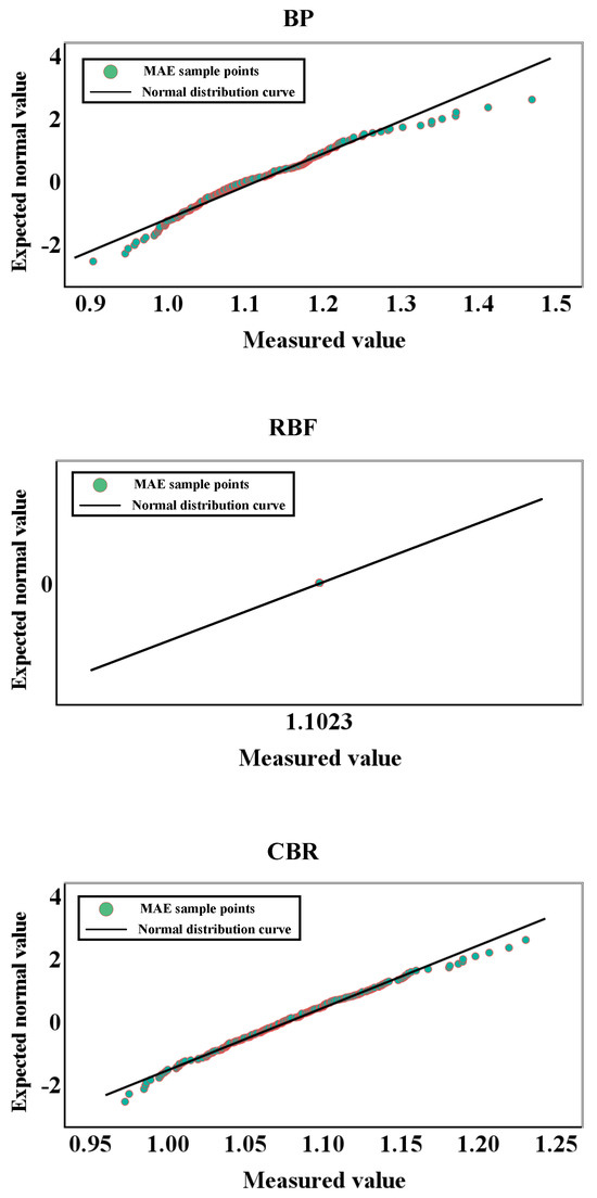
Figure 8.
Normal Q−Q plots for the MAE samples of the three models.
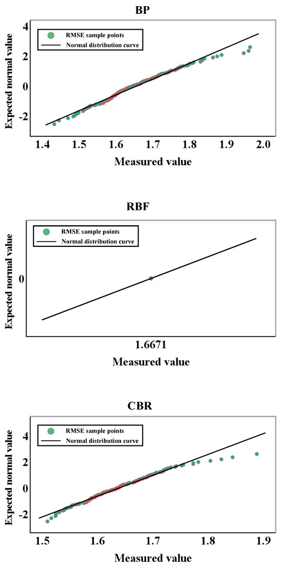
Figure 9.
Normal Q−Q plots for the three model RMSE samples.
Table 6.
Results of the K-S normal distribution tests for the MAE and RMSE samples for the three models.
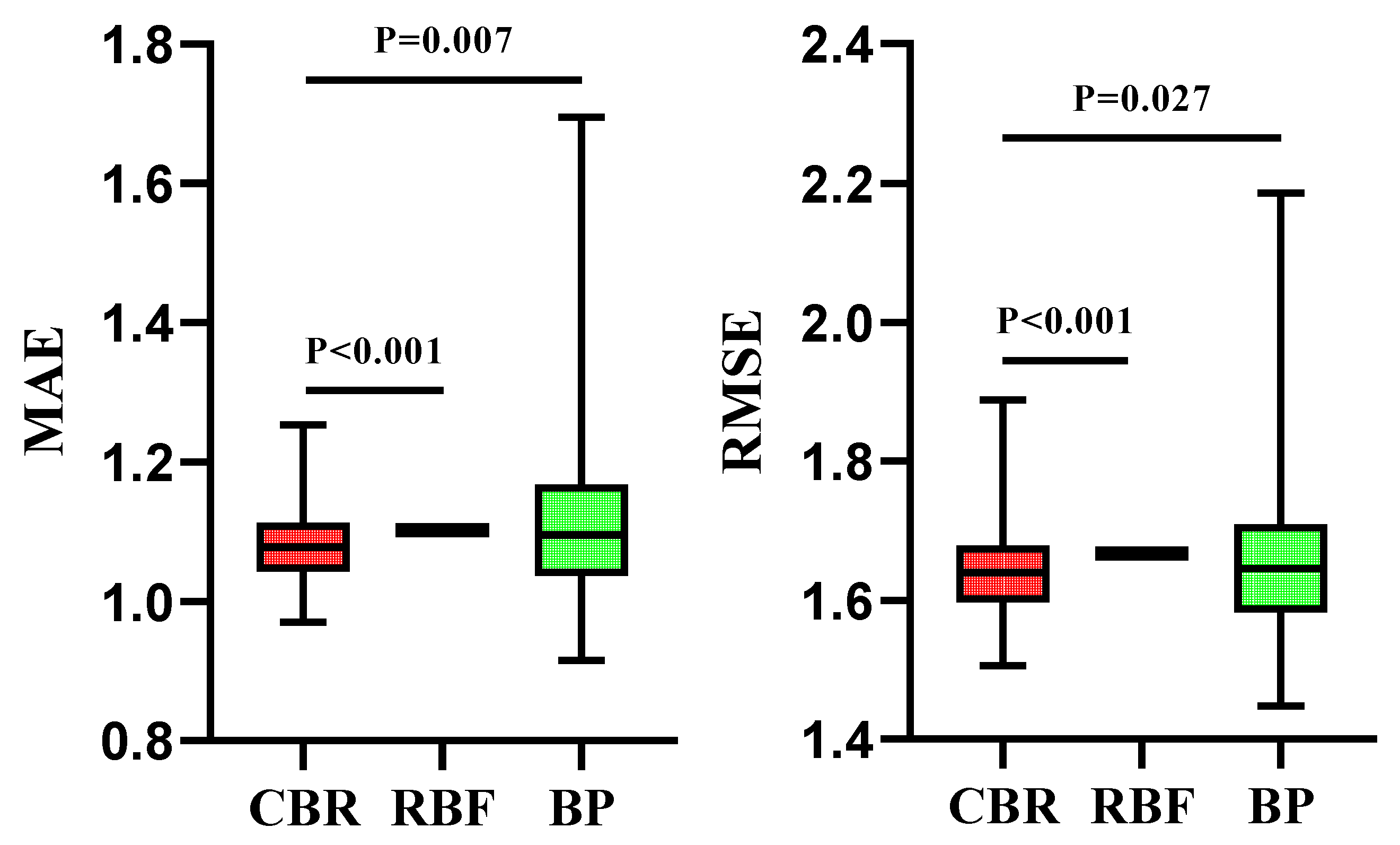
Table 6 indicates that in the MAE sample, only the CBR model exhibited a significant p-value exceeding 0.05 and conformed to a normal distribution. Thus, the independent sample median test was employed in the nonparametric analysis. In the RMSE sample, only the RBF model did not meet the normal distribution criteria. Therefore, an independent sample t-test was used for the CBR and BP models, while a nonparametric independent sample median test was applied to the CBR and RBF models. The nonparametric test and t-test assume that the CBR model is equivalent to the median and mean of the other models, respectively, and the null hypothesis is rejected when the significant p-value is below 0.05. Figure 10 illustrates the box plots of the MAE and RMSE samples for the three models, along with the significance test comparing the CBR model to the base model, with detailed findings included in Table 7.
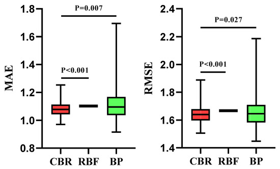
Figure 10.
CBR model vs. base model MAE and RMSE sample distributions and significant p-values.
Table 7.
Results of the sample hypothesis testing of the CBR model with the base model MAE and RMSE.
3.3. Resistance Prediction Results of the DTMB5415 Ship Type Based on an Improved WOA Algorithm
The resistance prediction of the constructed CBR model was executed using the improved WOA algorithm, which required an initial setup prior to commencement. The maximum number of iterations was set to 1000. According to Ref. [29], the whale population size N was set to 30, and the predation mechanism probability p was set to 0.5. Figure 11 illustrates the convergence plot of the optimization results of the WOA algorithm, which finally determined the optimal solution to be 140.6253. The X-axis denotes the number of iterations of the algorithm and the y-axis denotes the value of resistance to the algorithm’s search.
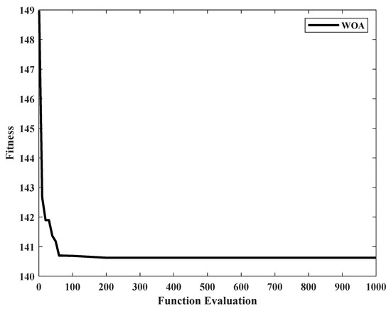
Figure 11.
Improved WOA algorithm searching for minimum resistance convergence iteration curves.
The results of the improved WOA were compared with four other intelligent optimization algorithms, namely, differential evolution (DE) [30], particle swarm optimization (PSO) [31], artificial bee colony (ABC) [32], and gray wolf optimization (GWO) [33], as well as a hybrid whale algorithm (HSMA_WOA) [34]. Figure 12 shows the results.
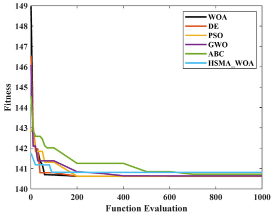
Figure 12.
Convergence curves of the improved WOA algorithm compared to other algorithms.
The CBR model and algorithm were run on a processor with a 12th Gen Intel® Core™ i7-12700H 2.30 GHz, 16 GB of RAM, and a Windows operating system, with MATLAB R2020b used as the testing software. The model and algorithm were trained using the CPU, with an average runtime of 35 s.
3.4. Comparison Results of the Optimized Ship Type and the Initial Ship Type
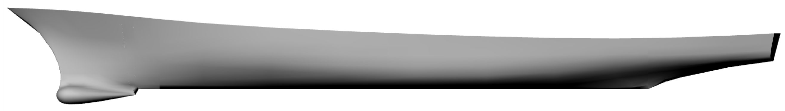
Table 8 shows the final geometric parameter values of the three design variables for the ball nose after optimization using the improved WOA algorithm. The results indicate that, compared to the original ship model, the optimized bulbous bow was augmented by 0.01997 in the x-direction and 0.00994 in the z-direction and increased by a factor of 1.5771 in the y-direction, resulting in an overall enlargement of the bulbous bow’s dimensions. Figure 13 illustrates a comparison between the initial DTMB5415 ship type and the optimized ship type hull in both front and side views.
Table 8.
Optimal values of the geometric parameters of the bulbous bow.
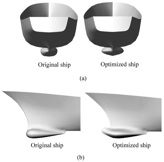
Figure 13.
Comparison of the front view and side view before and after optimization; (a) is the front view, (b) is the side view.
3.5. CFD Validation Results for Optimizing the Ship Resistance
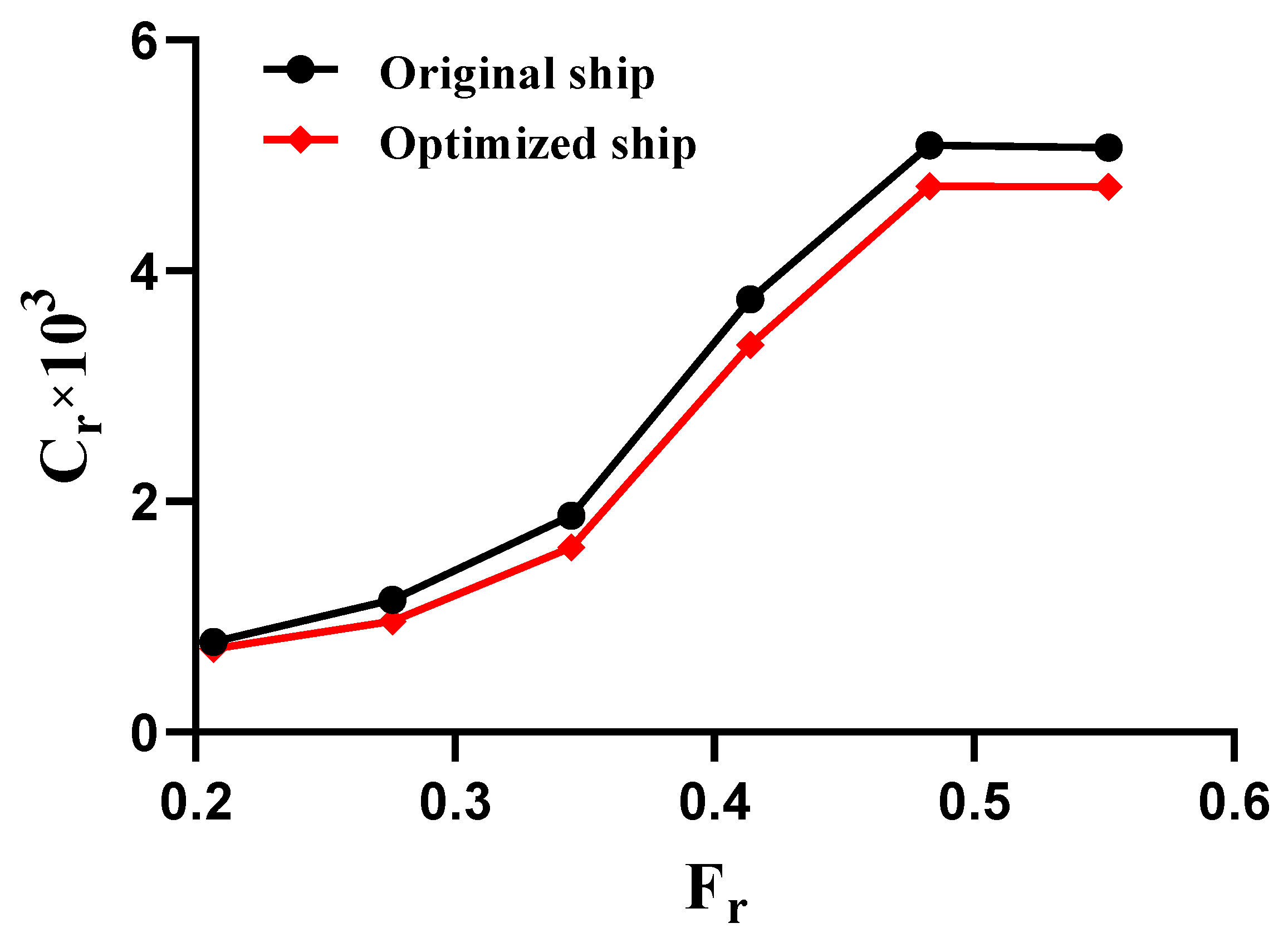
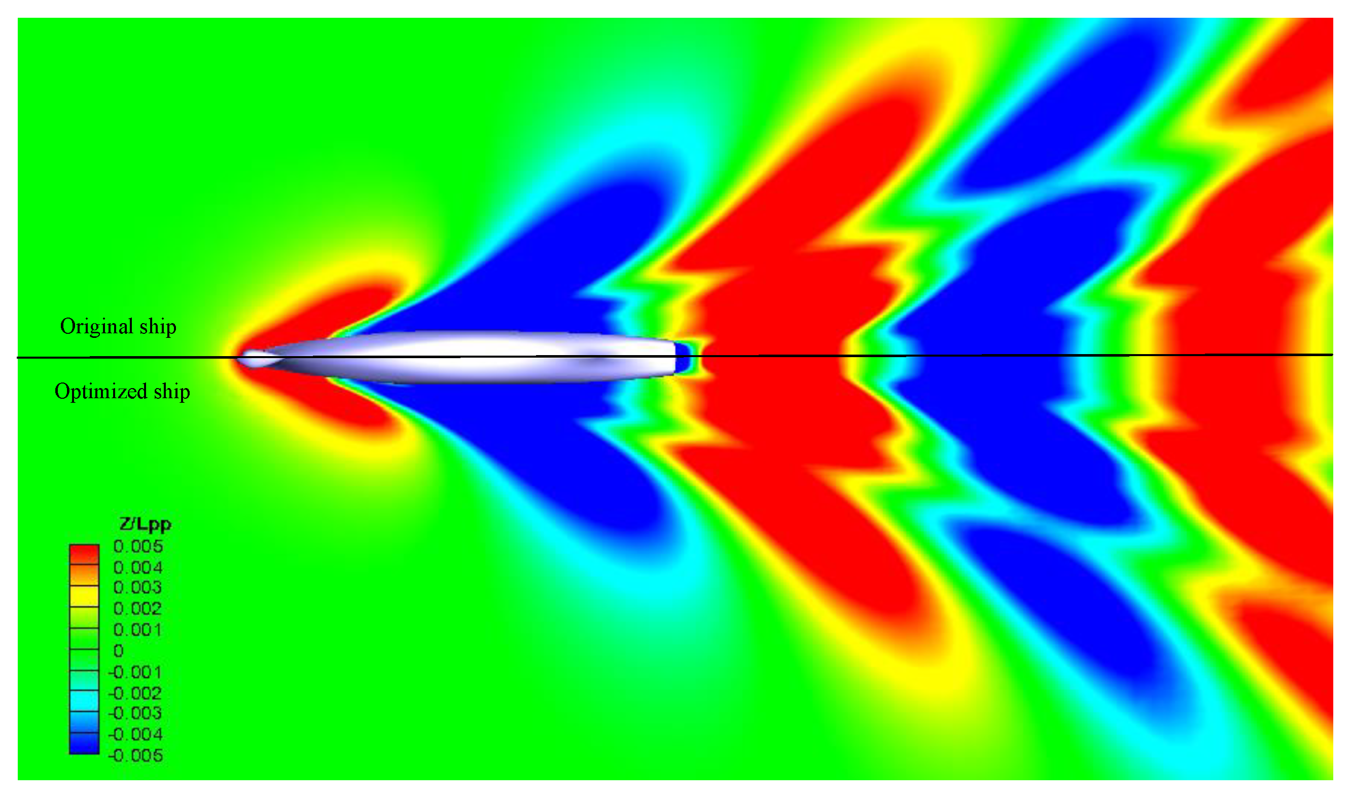
For the above-obtained results of the predicted resistance of the ship with a design speed of 30 knots and the Froude number , a series of parameters were verified for the optimal model of the ship using the CFD method; the results are shown in Table 9. The residual resistance coefficients and wave pattern for the optimized DTMB5415 ship type with a bulbous bow were computed at various speeds corresponding to and compared with the initial ship type, as shown in Figure 14 and Figure 15.
Table 9.
CFD validation results.
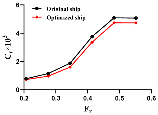
Figure 14.
Comparison of the residual drag coefficients between the initial and optimized ship models at different speeds corresponding to .
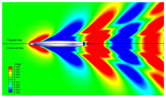
Figure 15.
Comparison of the wave patterns between the initial and optimized ship types.
The CFD simulation was run on a processor with an Intel® Xeon® Silver 4110 CPU 2.10 GHz, 128 GB of RAM, and a Windows operating system. The model was solved using the CPU, with an average CPU runtime of 6 h.
4. Discussion
Latin hypercube sampling divides each input dimension into equal intervals and randomly selects a point from each interval. This method ensures a uniform sample distribution within the input space, reducing bias and avoiding the unevenness of traditional random sampling. The results in Table 4 show that Latin hypercube sampling produces sample points with a greater average distance between them. Additionally, the variance in the distances to the nearest neighbors is lower than that of random sampling. This confirms that Latin hypercube sampling better represents the entire input space. This significantly affects the efficiency and accuracy of the subsequent WOA algorithm in identifying the minimum overall ship resistance of the model.
The prediction performance results of the three models indicated that the CBR model exhibited the lowest MAE relative to the BP and RBF models on the test set, with a 2.62% reduction in the median for both instances. This signifies that the CBR model exhibits the highest accuracy in forecasting the resistance. The CBR model showed impressive RMSE performance on the test set. It reduced the mean by 1.08% compared to the BP model and the median by 1.78% compared to the RBF model. This highlights the model’s stability and improved resilience. The box plots in Figure 10 indicate that the RBF model exhibits the highest stability, whereas the BP model demonstrates greater variability in accuracy but can attain a lower minimum. The CBR model integrates the strengths of both models, resulting in lower accuracy and commendable stability. Furthermore, the p-values for the CBR model compared to the RBF and BP models are all below 0.05, signifying a statistically significant difference in the MAE and RMSE between the CBR, RBF, and BP models.
The CBR model, due to its fast resistance prediction capability, can accurately design the ship’s structure based on real-time feedback to achieve optimal performance indicators. For example, the ship needs to consider indicators such as structural strength, propulsion efficiency, and fuel consumption. These indicators are closely related to the ship’s resistance. After designing a ship’s shape, the designer can use the CBR model to predict the resistance and immediately calculate the response of the above indicators. The ship’s shape can then be adjusted in real-time according to the requirements of actual production, without the need for hours of CFD simulations.
By using transfer learning to combine the training data of the DTMB5415 hull form with the design data of other hull forms, the CBR model can better transfer knowledge from the experience of one hull form to another, thereby reducing the amount of retraining required. When extending the surrogate model to other ship designs, it is necessary to map and normalize the input variables according to the geometric shape of the new hull form. Normalizing the design parameters ensures that the surrogate model has good generalizability across different hull forms.
The optimized bulbous bow extends outward along the centerline on both sides, transforming from a U-shape to a V-shape. Although the width is augmented, the bulbous bow appears flatter overall, facilitating a reduction in the wave resistance. The length of the bulbous bow is significantly increased, resulting in a longer inlet section below the waterline in the ship design, which may increase the friction resistance. However, this elongation also contributes to a decrease in the wave resistance, ultimately leading to a reduction in the total resistance, as wave resistance predominates in high-speed navigation. The optimized bulbous bow features an upturned tip, exhibiting a more pronounced slope alteration, whereas the bulbous bow of the original model remained predominantly at the level with minimal slope variation. The optimized bulbous bow design resulted in a 4.95% reduction in total resistance, a 7.14% reduction in the total resistance coefficient, and a 5.96% decrease in the effective power of the actual ship. Ref. [35] applied a gradient-based local optimization method to optimize the total resistance coefficient of the KCS ship, achieving a 1.8% improvement, which translated to a 3.1% reduction in effective power. In comparison, the method presented in this paper shows a significant improvement in the field of ship resistance prediction.
The residual resistance coefficient of the optimized bulbous bow is inferior to that of the initial ship model across various speeds, and the disparity is negligible when is below 0.3. The speed of the ship was low when was minimal, resulting in the friction resistance being predominant. Conversely, when is substantial, and the speed of the ship increases, the wave resistance becomes the primary factor, highlighting the effectiveness of the bulbous bow in reducing the resistance at this stage. Wave resistance typically increases linearly with velocity. The bulbous bow significantly reduces wave resistance, and changes in its shape have little effect on resistance at low speeds. The residual resistance coefficient curve indicates that the turning point for the DTMB5415 ship type occurs between . The bulbous bow of the lowest resistance ship type may have adverse effects when , as friction resistance predominates. The free-surface wave pattern diagrams indicate that the bow peak of the optimized vessel is marginally displaced forward, with the apex of the peak exhibiting a tendency to contract inward. The change is due to the optimized vessel’s elongated, flatter V-shaped bulbous bow. This design reduces the area from the bow tip to the peak of the wave, leading to a decrease in wave resistance around the vessel. The remainder of the area is consistent with the initial model; hence, the free-surface wave elevation of the optimized model remains largely unaltered following the second wave crest.
According to the results shown in Figure 12, the improved WOA algorithm exhibits the fastest convergence rate. The parameter helps the algorithm maintain a balance between model development and exploration processes, which enables the algorithm to converge quickly and find the global optimal solution in a short period of time. Simultaneously, the spiral update mechanism of the WOA algorithm allows for a progressive concentration on superior solutions within the search space, enhancing the convergence rate. The ABC method has the slowest convergence rate, owing to its reliance on extensive random searches facilitated by the exchange and transfer of information among various persons. The improved WOA algorithm has fewer core control parameters, including only population count, maximum iterations, and convergence factor. This reduces complexity and improves the efficiency of the search process. In contrast, the GWO algorithm includes these parameters as well as various classes of gray wolf populations, each associated with distinct convergence factors, resulting in a convergence speed surpassed only by the ABC algorithm.
In this study, the NURBS surface control points are used to model the bulbous bow, allowing for more localized modifications to the shape of the bow compared to using parameters such as radius, volume, and cross-sectional area. Ideally, each control point on the surface should be treated as an independent input parameter; however, an infinite number of control points would lead to the high-dimensional fitting problem in the surrogate model. Therefore, in this experiment, the overall coordinates of five sets of control points are selected as the input parameters for the model. In future work, the parametric representation of the curve can help reduce the dimensionality requirements to some extent.
The prediction results of the CBR model for optimization are generally consistent with those from the CFD simulations, although minor discrepancies still exist. The difference in the underlying principles between the two methods may be the cause of this discrepancy. CFD simulations model the interaction of the fluid with the ship’s surface to obtain resistance, dividing the hull into a large number of fine meshes to capture the mechanical characteristics of the fluid, which makes the results of CFD simulations very accurate. In contrast, the CBR model establishes a mapping relationship between hull parameters and ship resistance based on training data and constructs a specific mathematical model to predict ship resistance. Therefore, compared with CFD simulations, the CBR model tends to focus more on the overall trend for more complex nonlinear issues, with differences in detail. Training data are usually derived from CFD simulation results, and in practical scenarios, it is difficult to obtain resistance responses for all possible combinations of ship parameters. However, the CBR model offers significant advantages in terms of computational costs and time requirements. CFD simulations typically involve large computational loads, requiring substantial resources and time, whereas the CBR model allows for rapid predictions, thus improving production efficiency in practical engineering. For example, in this study, the CFD method takes up to 6 h to compute the results for a single sample. Ref. [16] also mentioned that using the viscous flow solver to solve the total resistance coefficient requires 175,000 s. In contrast, the CBR model offers significant advantages in computational cost and time, typically requiring only a few tens of seconds for iteration. This helps improve production efficiency in practical engineering applications. Although there are differences between the CBR model and CFD simulations, when the error requirements are met, this can be viewed as a trade-off between accuracy and speed.
This study examined the impact of bulbous bow design on resistance under ideal conditions. Excessively low resistance may indicate a non-traditional hull shape, which could adversely affect the ship’s seaworthiness and stability. When designing the hull, it is necessary to consider the balance between resistance and the economic efficiency of the ship. During navigation, environmental factors such as wind and sea waves also influence the total resistance of the hull, particularly during high-speed sailing, where these factors introduce additional constraints in resistance calculations. Consequently, predicting ship resistance under multiple constraints, along with multi-objective optimization of resistance and other performance metrics, is a promising direction for future research.
5. Conclusions
This study developed a surrogate model based on error classification and used the whale algorithm to analyze ship resistance with varying bulbous bow parameters. The method overcame the time-consuming and inefficient issues of traditional computational fluid dynamics (CFD). The main conclusions are as follows:
- The free-form deformation method converts hull surface deformation into the displacement of NURBS control point coordinates, offering a dependable approach for arbitrary ship alteration and delineating the essential parameters for generating the surrogate model.
- The CBR model can allocate the most appropriate prediction model for various sample points of the type of ship, resulting in superior overall performance in resistance prediction for the type of ship DTMB5415 compared to traditional neural networks BP and RBF.
- The improved whale algorithm demonstrates the fastest convergence among algorithms for identifying the optimal low-resistance ship type. This is due to the whale’s bubble net attack, which focuses on high-quality solution areas within the search space, leading to superior results in less time.
- The bulbous bow exhibiting the least resistance features an elongated forward section relative to the original design, while simultaneously being elevated. It was expanded by a factor of 1.5771 in width, transforming the overall configuration from a U-shape to a V-shape, thereby achieving a 4.95% decrease in the hull’s total resistance. The alteration in shape is predicated on a design velocity of 30 knots, where is equal to 0.4137.
Overall, the surrogate model proposed in this study provides a new approach for ship resistance prediction and lays the foundation for applying machine learning in bulbous bow design.
Author Contributions
Methodology, Y.S. and L.C.; data curation, Q.J. and B.J.; validation, Y.S. and B.J.; project administration, S.Y., Y.Z. and L.Q.; visualization, Q.J. and L.C.; writing—original draft preparation, Y.S.; writing—review and editing, S.Y., Y.Z. and L.Q. All authors have read and agreed to the published version of the manuscript.
Funding
This research was funded by (1) Research on the Mechanism of Hydrogen-Oxygen Flame Line Heating and Forming of Outer Hull Plate and Intelligent Operation Decision Support System (National Natural Science Foundation of China) grant number 51875270; (2) V-DT-driven and Al-enabled Comprehensive Protection Technology for Complex Equipment of Large Ships at Sea Research grant number JC2024021.
Institutional Review Board Statement
Not applicable.
Informed Consent Statement
Not applicable.
Data Availability Statement
The raw data supporting the conclusions of this article will be made available by the authors upon request.
Conflicts of Interest
The authors declare no conflicts of interest.
References
- Zhang, B. Research on ship hull optimisation of high-speed ship based on viscous flow/potential flow theory. Pol. Marit. Res. 2020, 27, 18–28. [Google Scholar]
- Wigley, W. The Theory of the Bulbous Bow and Its Practical Application; North East Coast Institution of Engineers and Shipbuilders: Newcastle-upon-Tyne, UK, 1936; pp. 52,65–88. [Google Scholar]
- Maruo, H.; Kasahara, K.; Miyazawa, M. Ship forms of minimum wave resistance with bulbs. J. Soc. Nav. Archit. Jpn. 1974, 1974, 13–24. [Google Scholar] [CrossRef]
- Baniela, S.I.; Díaz, Á.P. The first escort tractor Voith tug with a bulbous bow: Analysis and consequences. J. Navig. 2008, 61, 143–163. [Google Scholar] [CrossRef]
- El-Ela, A.M.A.; Hussien, M.M.; Elhadad, A.M. Bulbous Bow Shapes Effect on Ship Characteristics: A Review. J. Phys. Conf. Ser. 2024, 2811, 012012. [Google Scholar] [CrossRef]
- Lee, J.; Park, D.M.; Kim, Y. Experimental investigation on the added resistance of modified KVLCC2 hull forms with different bow shapes. Proc. Inst. Mech. Eng. Part M J. Eng. Marit. Environ. 2017, 231, 395–410. [Google Scholar] [CrossRef]
- Luo, W.; Lan, L. Design optimization of the lines of the bulbous bow of a hull based on parametric modeling and computational fluid dynamics calculation. Math. Comput. Appl. 2016, 22, 4. [Google Scholar] [CrossRef]
- Le, T.K.; He, N.V.; Hien, N.V.; Bui, N.T. Effects of a bulbous bow shape on added resistance acting on the hull of a ship in regular head wave. J. Mar. Sci. Eng. 2021, 9, 559. [Google Scholar] [CrossRef]
- Díaz Ojeda, H.R.; Oyuela, S.; Sosa, R.; Otero, A.D.; Pérez Arribas, F. Fishing Vessel Bulbous Bow Hydrodynamics—A Numerical Reverse Design Approach. J. Mar. Sci. Eng. 2024, 12, 436. [Google Scholar] [CrossRef]
- Jiang, X.; Lin, Y. Relevant integrals of NURBS and its application in hull line element design. Ocean Eng. 2022, 251, 111147. [Google Scholar] [CrossRef]
- Yang, Y.; Zhang, Z.; Zhao, J.; Zhang, B.; Zhang, L.; Hu, Q.; Sun, J. Research on Ship Resistance Prediction Using Machine Learning with Different Samples. J. Mar. Sci. Eng. 2024, 12, 556. [Google Scholar] [CrossRef]
- Tu, H.; Xia, K.; Zhao, E.; Mu, L.; Sun, J. Optimum trim prediction for container ships based on machine learning. Ocean Eng. 2023, 277, 111322. [Google Scholar] [CrossRef]
- Nazemian, A.; Boulougouris, E.; Aung, M.Z. Utilizing Machine Learning Tools for calm water resistance prediction and design optimization of a fast catamaran ferry. J. Mar. Sci. Eng. 2024, 12, 216. [Google Scholar] [CrossRef]
- Tran, T.G.; Van Huynh, Q.; Kim, H.C. Optimization strategy for planing hull design. Int. J. Nav. Archit. Ocean Eng. 2022, 14, 100471. [Google Scholar] [CrossRef]
- Zhang, S. Research on the deep learning technology in the hull form optimization problem. J. Mar. Sci. Eng. 2022, 10, 1735. [Google Scholar] [CrossRef]
- Liu, X.; Zhao, W.; Wan, D. Hull form optimization based on calm-water wave drag with or without generating bulbous bow. Appl. Ocean Res. 2021, 116, 102861. [Google Scholar] [CrossRef]
- Yongxing, Z.; Kim, D.J. Optimization approach for a catamaran hull using CAESES and STAR-CCM+. J. Ocean Eng. Technol. 2020, 34, 272–276. [Google Scholar] [CrossRef]
- Zhou, H.; Feng, B.; Liu, Z.; Chang, H.; Cheng, X. NURBS-Based Parametric Design for Ship Hull Form. J. Mar. Sci. Eng. 2022, 10, 686. [Google Scholar] [CrossRef]
- Sederberg, T.W.; Parry, S.R. Free-form deformation of solid geometric models. In Proceedings of the 13th Annual Conference on Computer Graphics and Interactive Techniques, Dallas, TX, USA, 18–22 August 1986; pp. 151–160. [Google Scholar]
- Nguyen Duy, T.; Hino, T. An improvement of interface computation of incompressible two-phase flows based on coupling volume of fluid with level-set methods. Int. J. Comput. Fluid Dyn. 2020, 34, 75–89. [Google Scholar] [CrossRef]
- Cakici, F.; Kahramanoglu, E. A RANS approach for transfer function plot based on discrete fourier transform. Ships Offshore Struct. 2022, 17, 1075–1086. [Google Scholar] [CrossRef]
- Senjanović, I.; Katavić, J.; Vukčević, V.; Vladimir, N.; Jasak, H. Launching of ships from horizontal berth by tipping tables–CFD simulation of wave generation. Eng. Struct. 2020, 210, 110343. [Google Scholar] [CrossRef]
- Gunaydinoglu, E.; Kurtulus, D.F. Pressure–velocity coupling algorithm-based pressure reconstruction from PIV for laminar flows. Exp. Fluids 2020, 61, 5. [Google Scholar] [CrossRef]
- Zheng, Y.; Lv, X.; Qian, L.; Liu, X. An optimal BP neural network track prediction method based on a GA–ACO hybrid algorithm. J. Mar. Sci. Eng. 2022, 10, 1399. [Google Scholar] [CrossRef]
- Harries, S.; Uharek, S. Application of radial basis functions for partially-parametric modeling and principal component analysis for faster hydrodynamic optimization of a catamaran. J. Mar. Sci. Eng. 2021, 9, 1069. [Google Scholar] [CrossRef]
- Kim, J.H.; Roh, M.I.; Kim, K.S.; Yeo, I.C.; Oh, M.J.; Nam, J.W.; Lee, S.H.; Jang, Y.H. Prediction of the superiority of the hydrodynamic performance of hull forms using deep learning. Int. J. Nav. Archit. Ocean Eng. 2022, 14, 100490. [Google Scholar] [CrossRef]
- Mirjalili, S.; Lewis, A. The whale optimization algorithm. Adv. Eng. Softw. 2016, 95, 51–67. [Google Scholar] [CrossRef]
- Ouyang, X.; Chang, H.; Feng, B.; Liu, Z.; Zhan, C.; Cheng, X. Information Matrix-Based Adaptive Sampling in Hull Form Optimisation. J. Mar. Sci. Eng. 2021, 9, 973. [Google Scholar] [CrossRef]
- Han, Q.; Yang, X.; Song, H.; Sui, S.; Zhang, H.; Yang, Z. Whale optimization algorithm for ship path optimization in large-scale complex marine environment. IEEE Access 2020, 8, 57168–57179. [Google Scholar] [CrossRef]
- Zhang, J.; Liu, M.; Zhang, S.; Zheng, R. AUV path planning based on differential evolution with environment prediction. J. Intell. Robot. Syst. 2022, 104, 23. [Google Scholar] [CrossRef]
- Ding, S.f.; Ma, Q.; Zhou, L.; Han, S.; Dong, W.b. Multipoint Heave Motion Prediction Method for Ships Based on the PSO-TGCN Model. China Ocean Eng. 2023, 37, 1022–1031. [Google Scholar] [CrossRef]
- Cao, H.; Zhang, J.; Cao, X.; Li, R.; Wang, Y. Optimized SVM-driven multi-class approach by improved ABC to estimating ship systems state. IEEE Access 2020, 8, 206719–206733. [Google Scholar] [CrossRef]
- Zhang, X.; Meng, Y.; Liu, Z.; Zhu, J. Modified grey wolf optimizer-based support vector regression for ship maneuvering identification with full-scale trial. J. Mar. Sci. Technol. 2022, 27, 576–588. [Google Scholar] [CrossRef]
- Abdel-Basset, M.; Chang, V.; Mohamed, R. HSMA_WOA: A hybrid novel Slime mould algorithm with whale optimization algorithm for tackling the image segmentation problem of chest X-ray images. Appl. Soft Comput. 2020, 95, 106642. [Google Scholar] [CrossRef] [PubMed]
- Park, S.W.; Kim, S.H.; Kim, Y.I.; Lee, I. Hull Form Optimization Study Based on Multiple Parametric Modification Curves and Free Surface Reynolds-Averaged Navier–Stokes (RANS) Solver. Appl. Sci. 2022, 12, 2428. [Google Scholar] [CrossRef]


Disclaimer/Publisher’s Note: The statements, opinions and data contained in all publications are solely those of the individual author(s) and contributor(s) and not of MDPI and/or the editor(s). MDPI and/or the editor(s) disclaim responsibility for any injury to people or property resulting from any ideas, methods, instructions or products referred to in the content. |
© 2025 by the authors. Licensee MDPI, Basel, Switzerland. This article is an open access article distributed under the terms and conditions of the Creative Commons Attribution (CC BY) license (https://creativecommons.org/licenses/by/4.0/).