Analysis of Optical Errors in Joint Fabry–Pérot Interferometer–Fourier-Transform Imaging Spectroscopy Interferometric Super-Resolution Systems

Abstract

Fourier-transform imaging spectroscopy (FTIS) faces inherent limitations in spectral resolution due to the maximum optical path difference (OPD) achievable by its interferometer. To overcome this constraint, we propose a novel spectral super-resolution technology integrating a Fabry–Pérot interferometer (FPI) with FTIS, termed multi-component joint interferometric hyperspectral imaging (MJI-HI). This method leverages the FPI to periodically modulate the target spectrum, enabling FTIS to capture a modulated interferogram. By encoding high-frequency spectral interference information into low-frequency interference regions through FPI modulation, an advanced inversion algorithm is developed to reconstruct the encoded high-frequency components, thereby achieving spectral super-resolution. This study analyzes the impact of primary optical errors and tolerance thresholds in the FPI and FTIS on the interferograms and spectral fidelity of MJI-HI, along with proposing algorithmic improvements. Notably, certain errors in the FTIS and FPI exhibit mutual interference. The theoretical framework for error analysis is validated and discussed through numerical simulations, providing critical theoretical support for subsequent instrument development and laying a foundation for advancing novel spectral super-resolution technologies.

1. Introduction

Fourier-transform imaging spectroscopy (FTIS) technology is based on the two-beam interference principle, where spectral information from the object plane is converted into an interferogram through optical Fourier transformation, and hyperspectral data are subsequently retrieved via interferogram inversion [1]. With the rapid advancement of spectroscopy, fields such as atmospheric environmental monitoring, water quality assessment, and mineral exploration increasingly demand higher spectral resolution from interferometric spectrometers [2,3,4,5,6,7]. In FTIS systems, spectral resolution is fundamentally determined by the maximum optical path difference (OPD), while the OPD sampling interval governs the operational spectral range. FTIS implementations can be categorized by modulation type: temporally modulated FTIS (TMFTIS), spatially modulated FTIS (SMFTIS), and temporally and spatially modulated FTIS (TSMFTIS). TMFTIS relies on the mechanical scanning of a moving mirror. TMFTIS imposes stringent requirements on the precision and stability of its moving mirror control system, making large-stroke reciprocating mirror motion challenging to implement [8,9,10]. To enhance the maximum effective OPD, researchers have employed cube-corner mirror motion to fold interference paths, thereby multiplying optical path lengths. However, this approach increases optical system complexity, introduces lateral shift and vibration-induced errors during mirror motion, and amplifies these errors with increasing folding cycles [11,12]. Additionally, novel interferometer designs—such as corner reflector interferometers, swing interferometers, and rotating parallel-mirror interferometers—have been proposed to reduce sensitivity to motion errors [13,14,15]. Nevertheless, constraints in uniformity, stability, and size/weight limitations further restrict the maximum achievable OPD. SMFTIS and TSMFTIS face inherent trade-offs between spectral resolution and coverage due to channel quantity limitations [1,16]. Although these systems exhibit superior mechanical stability, their relatively low resolution significantly hinders applications in high-precision remote sensing. Consequently, there is an urgent need for spectral super-resolution methods that maintain system stability and interferogram uniformity while remaining universally applicable to conventional FTIS architectures.

The Fabry–Pérot interferometer (FPI) operates on the principle of multi-beam interference and offers advantages such as compact size, high transmittance, strong spectral resolution, and structural stability, making it ideal for lightweight, high-precision hyperspectral imaging applications [17,18,19,20]. Beyond its traditional role as a spectral disperser, prior studies have integrated tunable FPIs into FTIS systems to enhance spectral resolution [21,22,23,24]. However, these approaches face challenges, including stringent requirements for cavity spacing tuning precision, prolonged spectral acquisition times, high costs, and difficulties in achieving large clear apertures, limiting their further development and practical application.

To address these limitations, we propose the multi-component joint interferometric hyperspectral imaging (MJI-HI) technique [25,26]. This method leverages a fixed-cavity, low-reflectivity FPI to modulate the object’s spectral information periodically. A dual-beam interferometer then performs an optical Fourier transformation on the modulated spectral signal to acquire the interferogram. The FPI’s modulation encodes high-frequency interference components (beyond the maximum OPD) into low-frequency interference regions. Through advanced inversion algorithms, these high-frequency components are separated and reconstructed, effectively extending the maximum OPD and thereby enhancing the spectral resolution of FTIS. The fixed-interval low-resolution FPI is used, which offers high stability, relaxed manufacturing and alignment precision requirements, and minimal error induction into FTIS systems. MJI-HI enhances spectral resolution by indirectly extending the maximum optical path difference (OPD), imposing no constraints on FTIS modulation schemes, sampling intervals, or spectral ranges. This demonstrates strong compatibility with FTIS architectures while delivering benefits including large optical throughput, structural simplicity, cost-effectiveness, and high robustness. The method is applicable to both SMFTIS and TSMFTIS. Furthermore, the system employs a dual-beam configuration to enhance spectral super-resolution accuracy while minimizing the potential system-level impacts introduced by FPI integration. We have proposed methods for twofold and multifold spectral super-resolution, and simulation analyses have verified the feasibility of achieving twofold and threefold spectral resolution enhancement. The future work will experimentally pursue higher super-resolution factors by holistically addressing FTIS stability, sampling strategies, inversion algorithm accuracy/efficiency, and FPI modulation techniques. However, there remains a lack of analysis regarding potential optical errors in MJI-HI and their impacts on system performance. Such investigations would establish a theoretical foundation for assessing the feasibility of higher-fold super-resolution schemes while providing critical guidance for MJI-HI’s further development and practical implementation.

Both FPI and FTIS are well-established interferometric systems, and their individual optical errors have been extensively studied [27,28,29,30,31,32,33,34]. However, despite prior research on combining FPI and FTIS, there remains a lack of systematic analysis of the optical errors in such integrated systems. Potential errors in the FPI include cavity spacing offsets, non-parallelism, surface irregularities, and reflectivity variations [27,28,29,30], while errors in the FTIS may involve mirror tilt, beam collimation accuracy, and beam splitter reflectivity variations [31,32,33,34]. This paper analyzes the impact of these errors on interferograms and spectral outputs, as well as their effects on the super-resolution results of MJI-HI. Based on the analysis, we propose algorithmic improvements to enhance system robustness. Additionally, the paper provides a detailed examination of interdependent errors between the FPI and FTIS, such as how FPI cavity spacing offsets interact with FTIS mirror tilt. The analysis is validated through simulation experiments. This work summarizes the critical technical considerations for developing MJI-HI and serves as a reliable reference for future studies integrating FPI and FTIS technologies.

2. Principles

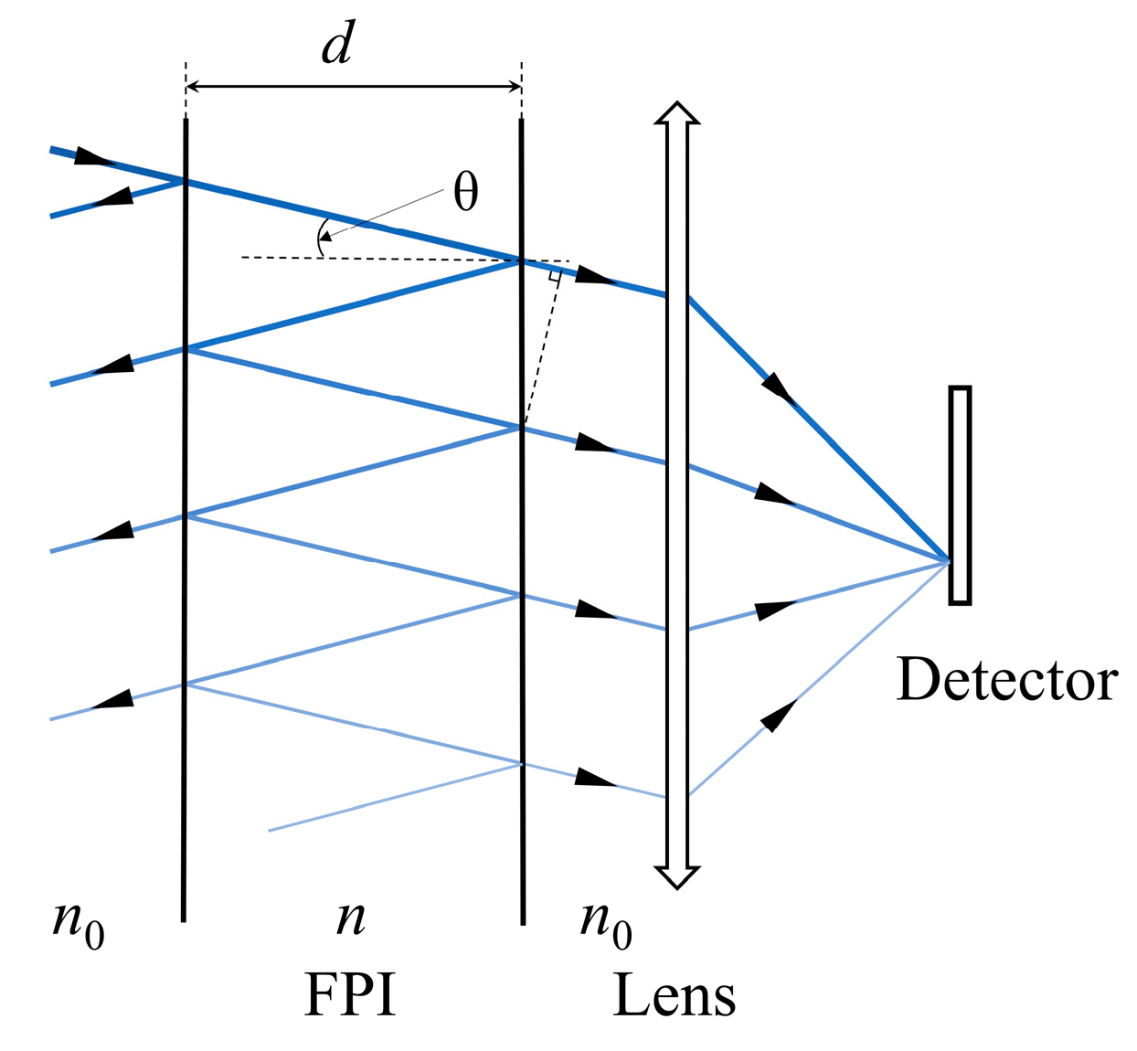
2.1. Principles of FPI

The FPI consists of two semi-reflective mirrors separated by a distance of d with a refractive index of n. Its schematic diagram is shown in Figure 1. A parallel beam with a wavenumber ν is incident on the FPI at an angle θ. After multiple reflections and transmissions, the exit angle of the light remains unchanged. The OPD between adjacent beams is Δ_FPI = 2ndcosθ, and the phase difference is δ_FPI = 4πνndcosθ.

The light beams exiting the FPI are converged onto the image plane by the imaging system, where multi-beam interference occurs. The effect of interference can be regarded as generating a transmission spectrum, with the FPI transmission spectrum T_FPI distributed as follows:

$$T_{FPI}\left(\nu \right)={\displaystyle \frac{{\left(1-R\right)}^2}{1+R^2-2R\cos \left(2\pi \nu {\Delta }_{FPI}\right)}}=a_0+{\displaystyle \sum _{m=1}^{\infty }2a_m\cos \left(m\cdot 2\pi \nu {\Delta }_{FPI}\right)},$$

(1)

where R denotes the reflectivity of the FPI reflective surface. The transmittance function T_FPI demonstrates periodicity in the wavenumber dimension and admits a Fourier series expansion. The coefficients are defined as follows: a₀ = (1 − R)/(1 + R) represents the DC component coefficient; a_m = R^m(1 − R)/(1 + R) corresponds to the fundamental frequency and higher-order harmonic coefficients.

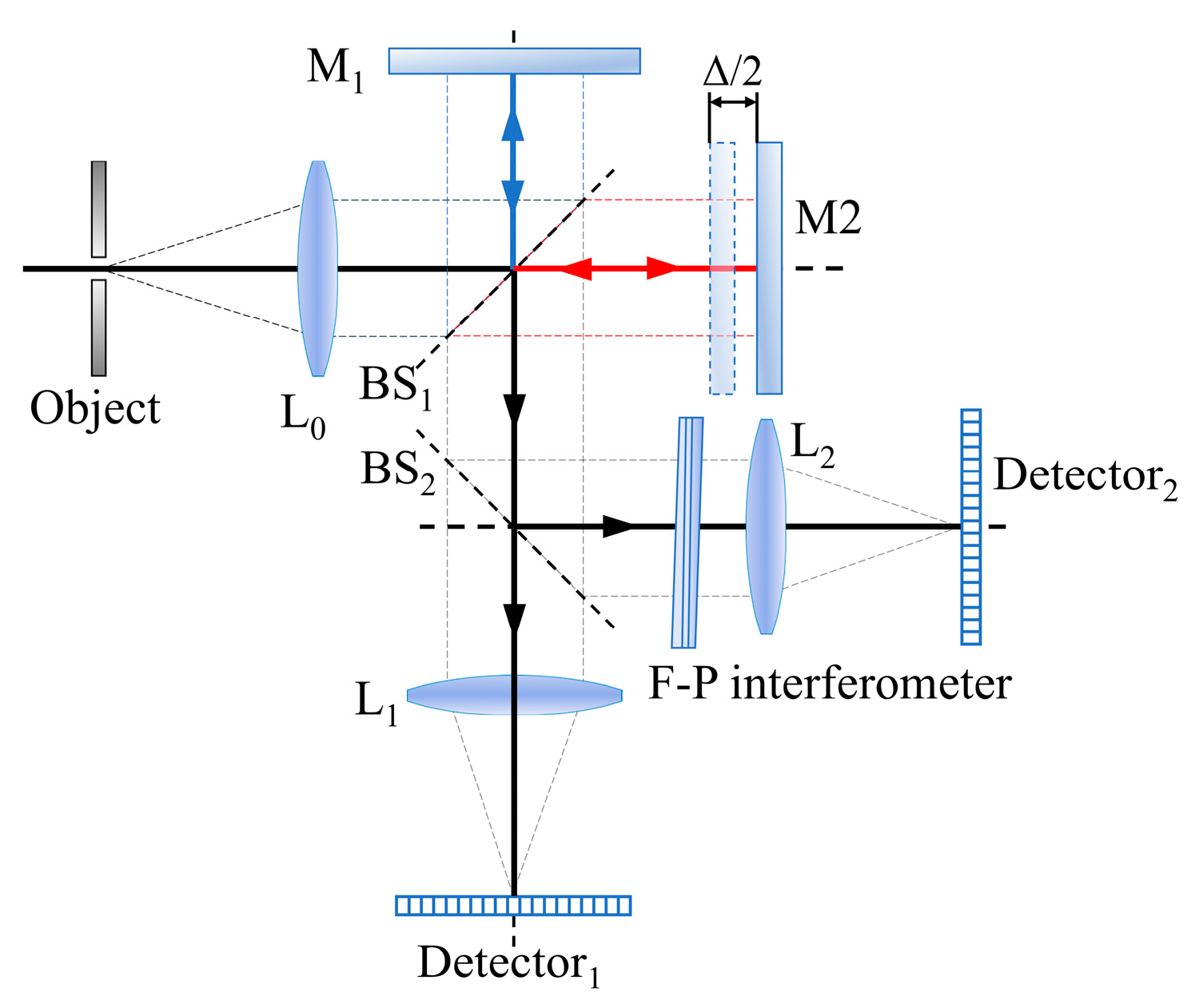
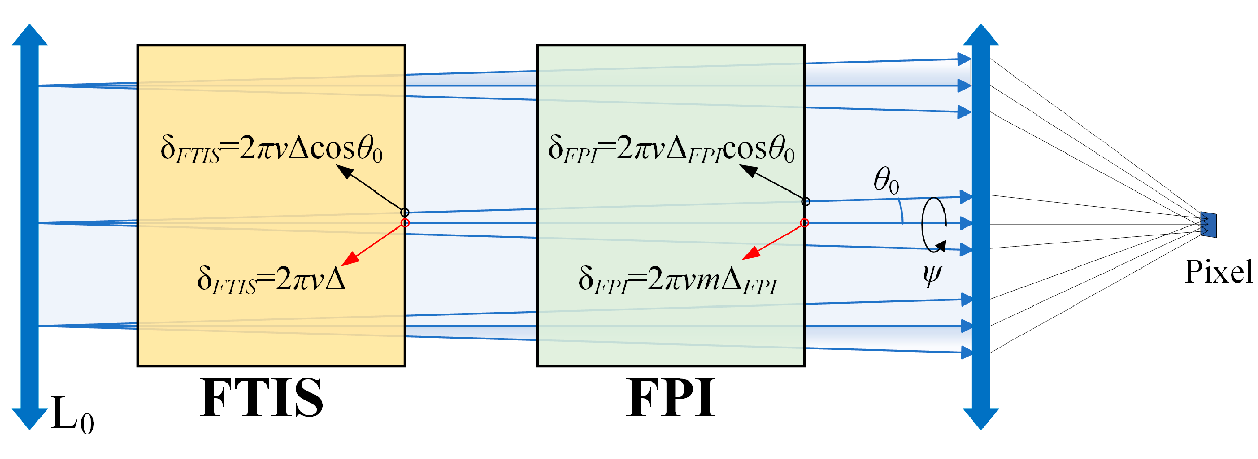
2.2. Principles of MJI-HI

The schematic diagram of the MJI-HI system principle based on TSMFTIS and FPI is shown in Figure 2, where system L₀ collimates the object beam into parallel light entering FTIS to generate two coherent beams with a defined OPD. A beam splitter then splits the emergent light into two optical paths: one beam converges through imaging system L₁ onto Detector₁, while the other first traverses the FPI before being focused by imaging system L₂ onto Detector₂, with both paths utilizing identical imaging systems and detectors differing only in the FPI’s presence. Assuming I₀ denotes the ideal interferogram spanning an OPD range of −∞ to +∞, Detector₁ acquires the FTIS interferogram I₁ constrained to an OPD range of [−L, L] (L being the maximum OPD of FITS), whereas Detector₂ captures the joint FTIS-FPI interferogram I₂ within the same OPD limits [−L, L]. The maximum OPD of interferograms I₁ and I₂ is governed by the maximum OPD of FTIS. Subsequent algorithmic processing synthesizes a new interferogram with doubled OPD range through computational integration of I₁ and I₂, thereby enabling spectral super-resolution via this hybrid optical–computational methodology.

The FTIS generates two coherent beams with a specific OPD, which propagate through L₁ and undergo two-beam interference upon imaging at Detector₁, where the resultant interferogram I₁ exhibits identical characteristics to those produced by conventional FTIS configurations.

$$I_1\left(\Delta \right)={\displaystyle \int R_{FTIS}{T}_{FTIS}B\left(v\right)\left[1+\cos \left(2\pi \nu \Delta \right)\right]} d\nu ,$$

(2)

where R_FTIS and T_FTIS denote the reflectivity and transmissivity of the FTIS beam splitter, respectively, ν is the wavenumber, and B(ν) represents the source spectral radiance. The OPD generated by the Michelson interferometer is defined as Δ = 2xcosθ, where x is the displacement of the moving mirror, and θ is the field angle. Neglecting the DC component, the interferogram I₁ can be expressed as follows:

$$I_1\left(\Delta \right)=FT\left[B\left(v\right)\right].$$

(3)

The finite OPD inherent in FTIS imposes fundamental constraints on system performance. Let L denote the maximum OPD, thereby defining the truncated interferogram as I₁(Δ) = I₀(Δ) for Δ ∈ (−L, L), where I₁(Δ) constitutes a windowed subset of I₀(Δ) restricted to this OPD range. This truncation results in the loss of high-frequency interference components beyond |Δ| > L, which directly limits the spectral resolution of TMFTIS systems.

In the alternate optical path, the two coherent beams emitted from FTIS propagate through the FPI. They are subsequently focused onto Detector₂ via imaging system L_2, simultaneously undergoing both two-beam and multiple-beam interference. The resultant composite interferogram arising from this joint interference mechanism can be expressed as follows:

$$\begin{array}{ll}{I}_2\left(\Delta \right)& ={\displaystyle \int B\left(v\right)T_{FPI}\left(v\right)\left[1+\cos \left(2\pi \nu \Delta \right)\right]} d\nu \\ & ={\displaystyle \int B\left(v\right)\left[1+\cos \left(2\pi \nu \Delta \right)\right]} \left[a_0+{\displaystyle \sum _{m=1}^{\infty }2a_m\cos \left(m\cdot 2\pi \nu {\Delta }_{FPI}\right)}\right]d\nu \end{array}.$$

(4)

The FPI employs a fixed cavity spacing d, maintaining a constant transmission function T_FPI(ν) throughout the FTIS scanning process. Consequently, the interferogram I₂ remains solely dependent on the OPD parameter Δ. By suppressing the DC component, the interferogram can be formulated as follows:

$$I_2\left(\Delta \right)=FT\left[B\left(v\right)T_{FPI}\left(v\right)\right]=I_0\left(\Delta \right)\ast FT\left[T_{FPI}\left(v\right)\right],$$

(5)

where ∗ denotes the convolution operator, and the joint interferogram fundamentally corresponds to the interferogram of B(ν)T_FPI(ν). By treating B(ν)T_FPI(ν) as an integrated spectral term (schematically represented in Figure 3a), the FTIS effectively performs an optical Fourier transform on this composite signal. Consequently, I₂ is mathematically equivalent to the convolution of the Fourier transform of FT[T_FPI(ν)] with the original interferogram I₀. Mirroring the constraints of I₁(Δ), the OPD range of I₂(Δ) remains bounded by Δ ∈ [−L, L], dictated by the FTIS’s maximum OPD.

In Equation (1), T_FPI(ν) can be expressed as comprising a DC component a₀, a fundamental frequency component 2a₁cos(2πνΔ_FPI), and higher-order harmonic components 2a_mcos(2πνmΔ_FPI). By combining Equation (1) with Equation (5), the derived relationship is as follows:

$$\begin{array}{ll}{I}_2\left(\Delta \right)& =I_0\left(\Delta \right)\ast \left\{a_0\delta \left(\Delta \right)+{\displaystyle \sum _{m=1}^{\infty }{a}_m\left[\delta \left(\Delta +m\cdot {\Delta }_{FPI}\right)+\delta \left(\Delta -m\cdot {\Delta }_{FPI}\right)\right]}\right\}\\ & =a_0{I}_0\left(\Delta \right)+{\displaystyle \sum _{m=1}^{\infty }{a}_m\left[I_0\left(\Delta +m\cdot {\Delta }_{FPI}\right)+I_0\left(\Delta -m\cdot {\Delta }_{FPI}\right)\right]}\end{array},$$

(6)

where δ represents the Dirac function. The presence of the DC component a₀ ensures that I₂(Δ) inherently contains the original interferogram I₀(Δ), where a₀I₀(Δ) is defined as the DC component of I₂(Δ). Simultaneously, the existence of fundamental and higher-order harmonic components introduces frequency-shifted interferometric terms I₀(Δ ± mΔ_FPI) into I₂(Δ), with a_mI₀(Δ ± mΔ_FPI) identified as the m-th order frequency-shifted component of I₂(Δ), where mΔ_FPI quantifies the frequency-shifted magnitude. Although the maximum OPD of I₂(Δ) remains confined to L, the incorporation of the FPI enables these frequency-shifted components to superimpose high-frequency information from I₀(Δ) beyond L onto I₂(Δ) via I₀(Δ ± mΔ_FPI), as schematically illustrated in Figure 3b. Consequently, the synergistic integration of I₁(Δ) and I₂(Δ) facilitates the reconstruction of I₀(Δ)’s high-frequency components through I₀(Δ ± mΔ_FPI), effectively extending the maximum OPD of I₀(Δ) and thereby enhancing spectral resolution by overcoming the Fourier uncertainty limit.

In Equation (6), the Fourier transform of the ideal FPI transmittance function, FT[T_FPI(ν)], can be rigorously expressed as a summation of δ functions. It is precisely the presence of these delta functions that ensures a strict linear relationship between the frequency-shifted components and I₀(Δ). These delta functions can be interpreted as the response functions of the I₂(Δ) DC component and frequency-shifted components with respect to I₀(Δ).

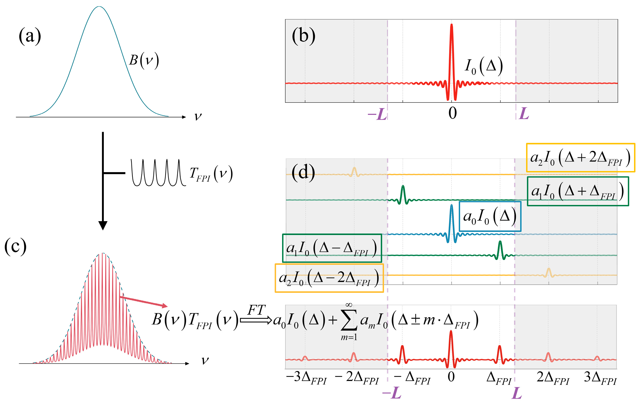
2.3. Inversion Algorithm

Building upon Equation (6), to encode the high-frequency information from the m = 1 order frequency-shifted component into the low-frequency regime of the fundamental component I₀(Δ), the FPI must satisfy Δ_FPI ≈ L. Typically, the amplitude of interferogram I₀(Δ) diminishes with increasing Δ, while the coefficients a_m progressively decrease at higher m values. Therefore, for the algorithmic simplification of Equation (6), components beyond m = 0, ±1, and 2 can be neglected within the Δ ∈ [0, L] domain due to their negligible energy contributions. Under this approximation, I₂(Δ) can be expressed as follows:

$$I_2\left(\Delta \right)=a_0{I}_0\left(\Delta \right)+{\displaystyle \frac{1}{2}}{a}_1{I}_0\left({\Delta }_{FPI}-\Delta \right)+{\displaystyle \frac{1}{2}}{a}_1{I}_0\left(\Delta +{\Delta }_{FPI}\right)+{\displaystyle \frac{1}{2}}{a}_2{I}_0\left(2{\Delta }_{FPI}-\Delta \right).$$

(7)

I₂(Δ) arises from the linear superposition of the DC component and frequency-shifted components. To reconstruct I₀(Δ), a system of linear equations relating I₀(Δ) to both I₁(Δ) and I₂(Δ) must be formulated. Based on Equation (7), the following linear system can be established.

$$\left[\begin{array}{c}{I}_1\\ I_2\end{array}\right]=\left[\begin{array}{cc}1& 0\\ A_1& A_2\end{array}\right]I_0=\mathsf{A}{I}_0.$$

(8)

In the equation, I₁, I₂ ∈ R^N represent N-dimensional column vectors composed of discrete data points from I₁(Δ) and I₂(Δ) over Δ ∈ [0, L], respectively. I₀ ∈ R^2N denotes a 2N-dimensional column vector constructed from I₀(Δ) across Δ ∈ [0, 2L]. The composite coefficient matrix A = [A₁ A₂]∈R^N×2N is derived from Equation (7), where A encapsulates the full-system coupling relationships. The computed I₀ enables twofold spectral super-resolution by effectively doubling the OPD range. To mitigate the ill-posed nature of this inverse problem, Equation (8) is reformulated as the following optimization framework:

$$\min {‖\mathsf{A}{I}_0-I‖}_2+\lambda {‖I_0‖}_2,$$

(9)

where I = [I₁; I₂] represents the vertically concatenated measurement vector, where ‖$\mathsf{A}$I₀ − I‖₂ constitutes the error term, and λ‖I₀‖₂ serves as the regularization term to mitigate ill-posedness and measurement uncertainties, with λ denoting the regularization coefficient that balances the error and regularization terms.

The system presented in this study achieves a twofold extension of the maximum OPD for I₀ through the synergistic utilization of two interferograms I₁ and I₂, thereby achieving twofold spectral super-resolution. Theoretically, this approach can be extended by implementing additional optical paths or utilizing tunable FPIs to acquire more interferograms, thereby enabling threefold or multifold spectral super-resolution through the establishment of higher-dimensional linear systems of equations using the same data processing procedure as applied to I₂.

3. Optical Error Analysis

The theoretical analysis in Section 2 is based on the idealized assumptions of FTIS and FPI performance. However, in practical implementations, positional and alignment errors in optical components within the FTIS and FPI systems inevitably introduce deviations between measured data and theoretical predictions. The foundational principle of MJI-HI relies on establishing a linear relationship between I₂ and I₀ in Equation (6) through FPI modulation, which enables the reconstruction of the original interferogram via this linear dependency. It is, therefore, critical to systematically evaluate whether these optical errors compromise the integrity of this linear relationship. In the interferogram I₂, the frequency-shifted components can be expressed as follows: a_mI₀(Δ ± mΔ_FPI) = I₀(Δ) ∗ a_mδ(Δ ± mΔ_FPI). Here, a_mδ(Δ ± mΔ_FPI) serves as the response function for each frequency-shifted component. Analyzing the deviations caused by various optical errors in the response function provides a more intuitive understanding of their impact on the linear relationship and the overall effect on each frequency-shifted component. In the following sections, the interferograms I₀, I₁, and I₂ under different error conditions are denoted as I_0-error, I_1-error, and I_2-error, respectively.

3.1. Optical Errors of FPI

The main errors in the FPI include optical path errors, non-parallelism errors, non-flatness errors, and coating reflectance errors. The FPI optical path length determines the frequency-shift positions of spectral components; deviations in this parameter directly affect the construction of the coefficient matrix A. Non-parallelism and surface irregularities induce spatially dependent OPD variations across the clear aperture, thereby perturbing the linear relationship defined in Equation (8). Wavelength-dependent fluctuations in the semi-reflective coating’s reflectivity alter the harmonic coefficients a_m and further compromise the system’s linearity. This section provides a detailed analysis of these error mechanisms and proposes corresponding algorithmic enhancements to mitigate their impacts.

3.1.1. Optical Path Difference Error

The frequency-shifted magnitude mΔ_FPI is fundamentally determined by the cavity spacing d, incidence angle θ, and refractive index n. Multiple factors influence d, including assembly tolerances, reflective coating thickness variations, and temperature fluctuations; θ is predominantly affected by the tilt angle of FPI components perpendicular to the optical axis; n exhibits susceptibility to environmental variations such as temperature and pressure changes. These imperfections collectively induce drift in mΔ_FPI. MJI-HI leverages the FPI to generate frequency-shifted components, establishing a linear relationship between interferograms and I₀ to reconstruct high-frequency interference information. Within this framework, Δ_FPI serves as a critical parameter in formulating the linear relationship defined in Equation (8). To enable Δ_FPI computation and dynamic calibration, Δ_FPI must be slightly smaller than L, ensuring I₂(Δ) encapsulates I₂(Δ_FPI). As the interferogram I₀ corresponds to the Fourier transform of the spectrum, its energy is predominantly concentrated in the low-frequency region near Δ = 0. Consequently, Equation (6) can be approximated as follows:

$$\left\{\begin{array}{l}{I}_2\left[U\left(0\right)\right]\approx a_0{I}_0\left[U\left(0\right)\right]\\ I_2\left[U\left(\pm {\Delta }_{FPI}\right)\right]\approx a_1{I}_0\left[U\left(0\right)\right]\end{array}\right.,$$

(10)

where U(Δ) denotes the neighborhood of Δ. The value of Δ_FPI can be determined by computing the cross-correlation I₂[U(0)] ⊗ I₂[U(±Δ_FPI)] and identifying the position of maximum correlation, where ⊗ represents the cross-correlation operator. This methodology enables the real-time correction of Δ_FPI when cavity spacing variations occur in the FPI, thereby preserving the accuracy of the linear system formulation.

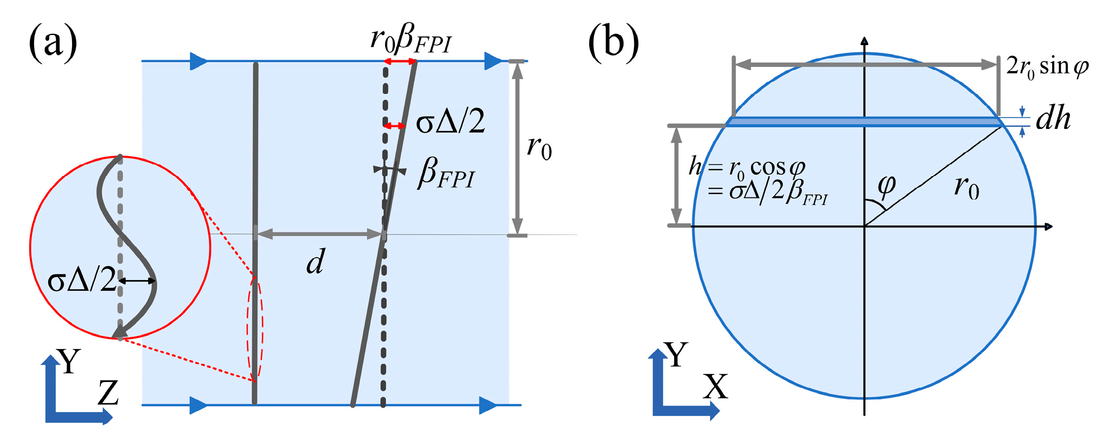
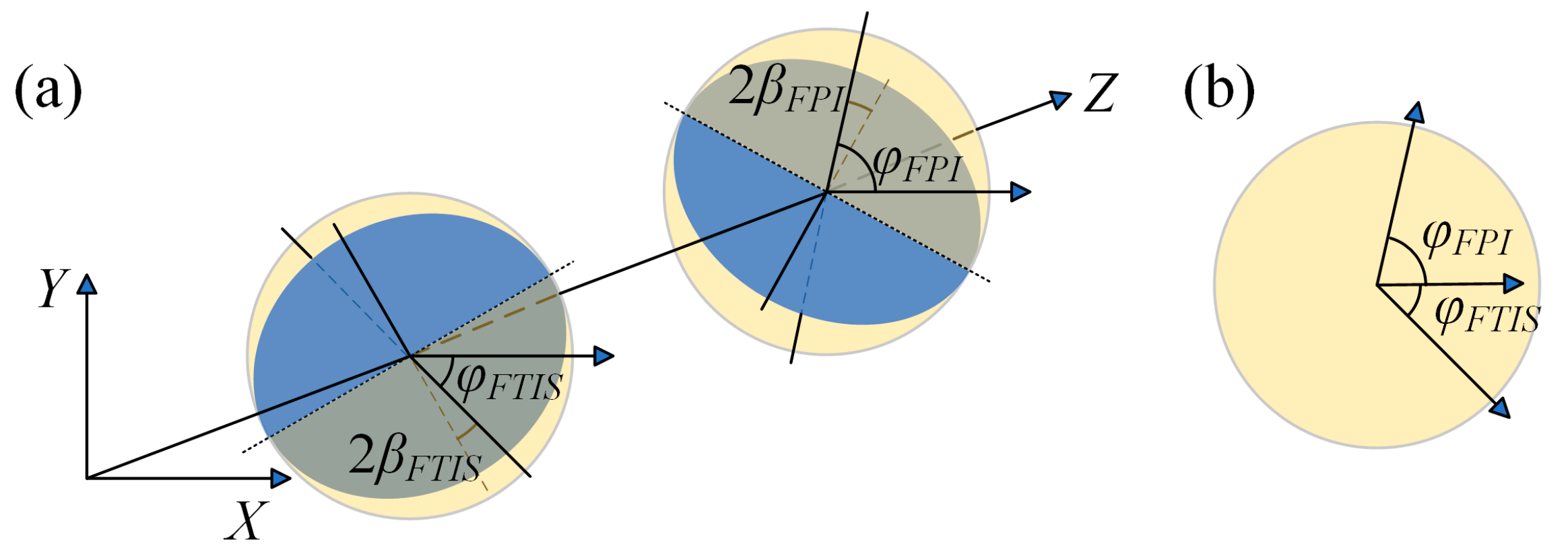
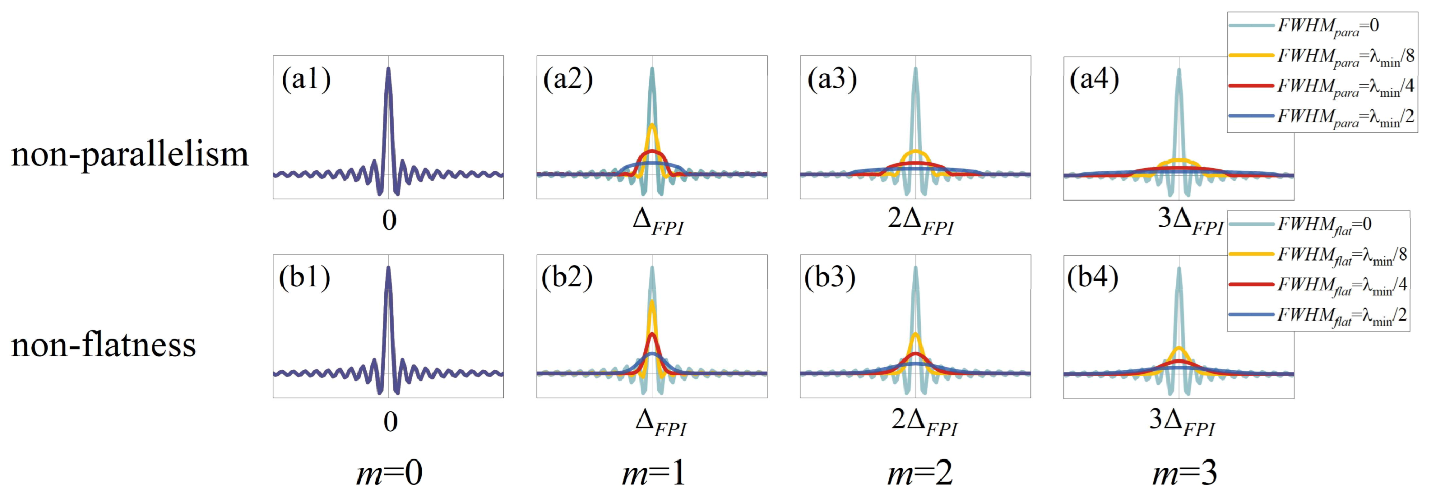
3.1.2. Non-Parallelism Error of FPI

During the manufacturing and alignment processes of the FPI, a small angular deviation β_FPI between the two partially reflective surfaces introduces position-dependent OPD variations across the aperture. As shown in Figure 4, it should be assumed that one of the semi-reflective surfaces of the FPI tilts along the Y-axis direction. The aperture is circular with a radius of r₀, and the cavity length error introduced by the non-parallelism is σΔ/2, resulting in an optical path error of σΔ. The normalized distribution function of the OPD error is as follows:

$$g_{FPI}\left(\sigma \Delta \right)={\displaystyle \frac{1}{\pi {\beta }_{FPI}{r}_0}}\sqrt{1-{\left(\sigma \Delta /2{\beta }_{FPI}{r}_0\right)}^2}.$$

(11)

In the equation, r denotes the radius of the clear aperture. From Equation (11), we further derive the full width at the half maximum of g_FPI(σΔ) as FWHM_para = $2\sqrt{3}$β_FPIr₀. A point on the aperture at a height along the Y-axis can be expressed as h = σΔ/2β_FPI, where β_x is the tilt angle. Let σΔ = 2β_FPIr₀cosφ, as shown in Figure 4, where φ is the azimuthal angle. Integrating over the entire aperture, the FPI’s transmission spectrum is as follows:

$$\begin{array}{ll}{T}_{FPI-para}\left(\nu \right)& ={\displaystyle {\int }_{-2{\beta }_{FPI}{r}_0}^{2{\beta }_{FPI}{r}_0}{T}_{FPI}\left(v,{\Delta }_{FPI}+\sigma \Delta \right)g\left(\sigma \Delta \right)d(\sigma \Delta )}\\ & =a_0+{\displaystyle {\int }_0^{\pi }{\displaystyle \sum _{m=1}^{\infty }\frac{2a_m}{\pi }}\cos \left[2\pi vm\left({\Delta }_{FPI}+2{\beta }_{FPI}{r}_0\cos \phi \right)\right]{\sin }^2\phi d\phi }\\ & =a_0+{\displaystyle \sum _{m=1}^{\infty }{a}_m\frac{2J_1\left(2\pi \nu m2r_0{\beta }_{FPI}\right)}{2\pi \nu m2r_0{\beta }_{FPI}}\cos \left(2\pi \nu m{\Delta }_{FPI}\right)}\end{array},$$

(12)

where J₁(z) denotes the first-order Bessel function of the first kind. The impact of non-parallelism errors on the transmission spectrum of the Fabry–Pérot interferometer (FPI) is illustrated in Figure 5. Overall, such errors cause a certain degree of reduction in the interference intensity of T_FPI-para. By decomposing the transmission spectrum into DC components, fundamental frequency components, and higher-order harmonic components, as shown in Figure 5b–e, it is observed that under ideal conditions, the fundamental and higher-order harmonic components exhibit standard cosine functions. However, non-parallelism errors lead to a decrease in the interference intensity of each component. Moreover, as the order m and wavenumber ν increase, the attenuation of interference intensity becomes more pronounced. Additionally, non-parallelism errors do not cause changes in the periodic frequency of the harmonic components.

According to Equation (6), the influence on the interferogram is as follows:

$$\begin{array}{ll}{I}_{2-para}\left(\Delta \right)& ={\displaystyle {\int }_{-2{\beta }_{FPI}{r}_0}^{2{\beta }_{FPI}{r}_0}{I}_0\left(\Delta \right)\ast FT\left[T_{FPI}\left(\nu ,{\Delta }_{FPI}+\sigma \Delta \right)\right]}g\left(\sigma \Delta \right)d\sigma \Delta \\ & =I_0\left(\Delta \right)\ast \left\{a_0\delta \left(\Delta \right)+{\displaystyle \sum _{m=1}^{\infty }{a}_m\left[\delta \left(\Delta +m{\Delta }_{FPI}\right)+\delta \left(\Delta -m{\Delta }_{FPI}\right)\right]}\ast g_m\left(\Delta \right)\right\}\\ & =a_0{I}_0\left(\Delta \right)+{\displaystyle \sum _{m=1}^{\infty }{a}_m\left[I_0\left(\Delta +m{\Delta }_{FPI}\right)+I_0\left(\Delta -m{\Delta }_{FPI}\right)\right]}\ast g_m\left(\Delta \right)\end{array}.$$

(13)

In the equation, g_m(Δ) = g(Δ/m)/m. Consequently, compared to Equation (6), FPI non-parallelism introduces a convolution of frequency-shifted components response function a_mδ(Δ ± mΔ_FPI) with g_m(Δ), resulting in response function broadening where the broadening width increases by a factor of m and the amplitude reduces to 1/m as the harmonic order m increases. Notably, this effect does not influence the DC component a₀I₀(Δ), as the DC term remains unaffected by the angular misalignment-induced broadening mechanism.

3.1.3. Non-Flatness Error of FPI

Surface imperfections inherent in fabricating FPI partially reflective surfaces induce position-dependent OPD across the clear aperture, as indicated by σΔ in Figure 4. The normalized distribution of OPD errors resulting from these non-flatness error can be expressed as follows:

$$p\left(\sigma \Delta \right)={\displaystyle \frac{1}{\sqrt{\pi }\sigma {\Delta }_D}}{e}^{-{\displaystyle \frac{\sigma {\Delta }^2}{\sigma {\Delta }_D^2}}},$$

(14)

where σΔ_D denotes the surface defect factor. Following Equation (14), the FWHM of p(σΔ) is expressed as FWHM_flat = $2\sqrt{ln2}$σΔ_D. The transmission function of the FPI can then be formulated as follows:

$$\begin{array}{ll}{T}_{FPI-flat}\left(\nu \right)& ={\displaystyle {\int }_{-\infty }^{\infty }{T}_{FPI}\left(v,{\Delta }_{FPI}+\sigma \Delta \right)p\left(\sigma \Delta \right)d(\sigma \Delta )}\\ & =a_0+{\displaystyle \sum _{m=1}^{\infty }2a_m\cos \left(2\pi vm{\Delta }_{FPI}\right)\ast p\left({\Delta }_{FPI}\right)}\\ & =a_0+{\displaystyle \sum _{m=1}^{\infty }2a_m{e}^{-\left(\pi m\sigma {\Delta }_D\nu \right)}\cos \left(2\pi vm{\Delta }_{FPI}\right)}\end{array}.$$

(15)

Consequently, the non-flatness error induces Gaussian smoothing of the transmission spectrum T_FPI (ν) through convolution with a Gaussian kernel p(σΔ), as shown in Figure 6. When T_FPI-flat is decomposed into its DC component and various harmonic components, its effect is similar to that of non-parallelism error. The interference intensity of each harmonic component decreases, which can be regarded as producing an interference intensity factor of exp[−(mπσΔ_Dν)²]. Therefore, as the order m and the wavenumber ν increase, the interference intensity decreases more dramatically.

Accounting for this imperfection, the joint interferogram can be expressed as follows:

$$\begin{array}{ll}{I}_{2-flat}\left(\Delta \right)& ={\displaystyle {\int }_{-\infty }^{\infty }{I}_0\left(\Delta \right)\ast FT\left[T_{FPI}\left(v,{\Delta }_{FPI}+\sigma \Delta \right)\right]p\left(\sigma \Delta \right)d\sigma \Delta }\\ & =I_0\left(\Delta \right)\ast \left[a_0\delta \left(\Delta \right)+{\displaystyle \sum _{m=1}^{\infty }{a}_m\left[\delta \left(\Delta +m{\Delta }_{FPI}\right)+\delta \left(\Delta -m{\Delta }_{FPI}\right)\right]}\ast p_m\left(\Delta \right)\right]\\ & =a_0{I}_0\left(\Delta \right)+{\displaystyle \sum _{m=1}^{\infty }{a}_m\left[I_0\left(\Delta +m{\Delta }_{FPI}\right)+I_0\left(\Delta -m{\Delta }_{FPI}\right)\right]}\ast p_m\left(\Delta \right)\end{array},$$

(16)

where p_m(Δ) = p (Δ/m)/m. Consequently, analogous to the effects of non-parallelism, FPI non-flatness error causes the frequency-shifted component response function to convolve and broaden, resulting in a_mδ(Δ ± mΔ_FPI) ∗ p_m(Δ). The width and height of the broadening are both related to the order m.

Based on the above analysis, the effects of FPI non-parallelism and non-flatness on the interferogram can be regarded as two equivalent errors. By combining these two defects, the total error interferogram can be expressed as follows:

$$\left\{\begin{array}{ll}{I}_{2-flat}\left(\Delta \right)& =I_0\left(\Delta \right)\ast \left[a_0\delta \left(\Delta \right)+{\displaystyle \sum _{m=1}^{\infty }{a}_m\delta \left(\Delta \pm m{\Delta }_{FPI}\right)}\ast Defec{t}_m\left(\Delta \right)\right]\\ & =a_0{I}_0\left(\Delta \right)+{\displaystyle \sum _{m=1}^{\infty }{a}_m}{I}_0\left(\Delta \pm m\cdot {\Delta }_{FPI}\right)\ast Defec{t}_m\left(\Delta \right)\\ Defec{t}_m\left(\Delta \right)& ={\mathrm{g}}_m\left(\Delta \right)\ast p_m\left(\Delta \right)\end{array}\right..$$

(17)

Compared to Equation (6), the response function of the frequency-shifted component becomes a_mδ(Δ ± mΔ_FPI) ∗ Defect_m(Δ). If the width of Defect_m(Δ) remains relatively small, the combined effects of these two defect types can be neglected; otherwise, an enhanced model must be developed to account for these imperfections. In practical FPI manufacturing, non-parallelism and surface irregularities in fixed-spacing FPIs can typically be quantified through metrological techniques, allowing the theoretical profile of Defect_m(Δ) to be treated as a priori knowledge. The term a_mDefect_m(Δ) can thus be expressed in the vector form as a_m-Defect∈R ^з, where з denotes the dimensionality of a_m-Defect determined by the width of Defect_m(Δ). This vectorized representation enables the simulation of the convolutional effects induced by Defect_m through the substitution of a_m-Defect for the original coefficient a_m in the system matrix A of Equation (8).

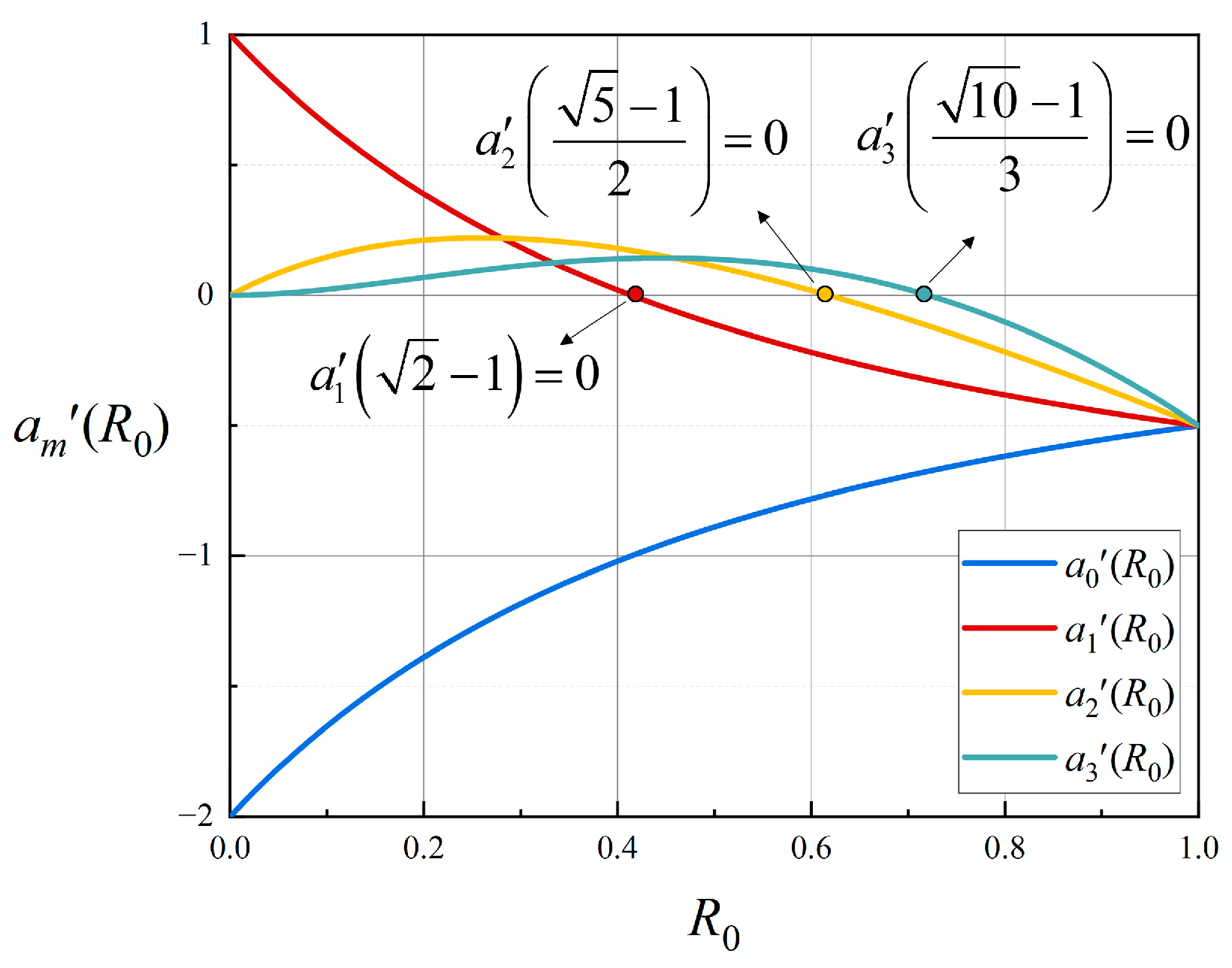
3.1.4. Reflectivity Changes in FPI

In ideal FPI configurations, the reflectivity R of semi-reflective surfaces is typically treated as a constant value. However, practical implementations exhibit wavelength-dependent reflectivity variations expressed as R(ν) = R₀ + δR(ν), where R₀ represents the mean reflectivity, and δR(ν) denotes the spectral deviation term. This variation primarily affects the harmonic coefficients a_m, which can be reformulated through Taylor expansion about R₀ as follows:

$$\begin{array}{l}{a}_m\left(\nu \right)=a_m+{a^{\prime }}_m\delta R\left(\nu \right)+o\left[\delta R{\left(\nu \right)}^n\right]\\ \left\{\begin{array}{l}{a}_m=R_0^m{\displaystyle \frac{1-R_0}{1+R_0}}\\ {a^{\prime }}_m={\displaystyle \frac{R_0^{m-1}\left[m\left(1-R_0^2\right)-2R_0\right]}{{\left(1+R_0\right)}^2}}\end{array}\right.\end{array}.$$

(18)

In the equation, the influence of reflectivity variations on the coefficients is denoted by a′_mδR(ν). The a′_m is the first derivative of a_m with respect to R₀, and it quantitatively represents the sensitivity of a_m to changes in reflectivity. From the analytical expression of a′_m, the functional dependencies of a′₀, a′₁, a′₂, and a′₃ on R₀ can be derived and plotted as characteristic curves, as shown in Figure 7. For the MJI-HI system achieving twofold spectral super-resolution, the dominant contributions originate from the m = 0 and 1 frequency-shifted components, whereas multifold super-resolution necessitates the inclusion of higher-order terms (m ≥ 2), each successively introducing finer spectral modulation through harmonic interference coupling proportional to its respective sensitivity coefficients a′_m.

For the m = 0 order, the sensitivity coefficient is given by a′₀ = −2/(1 + R₀)², with its value ranging from −2 to −0.5. As R₀ increases, the influence of reflectivity variations on a₀(ν) diminishes. For the m = 1 order, a′₁ = 0 when R₀ =−1 = 41.4%, rendering the coefficient minimally sensitive to small reflectivity fluctuations. Similarly, for the m = 2 order, a′₂ = 0 at R₀ = ($\sqrt{5}$ − 1)/2 = 61.8%. However, it is fundamentally impossible to simultaneously nullify the sensitivity of all m-order frequency-shifted components to δR(ν). For twofold spectral super-resolution, selecting an FPI with R₀ ≈ 41.4% effectively reduces the sensitivity of a₁. For threefold super-resolution, FPIs with R₀ ∈ [41.4%, 61.8%] achieve concurrently low sensitivity for both a₁ and a₂, thereby optimizing performance across multiple harmonic orders while maintaining robustness against reflectivity variations.

Taking R₀ = 40% as an example, a randomly generated reflectance variation curve δR(ν) is introduced. Under this error condition, the variations in the FPI transmission spectrum T_FPI-R and its constituent components are illustrated in Figure 8. Overall, the reflectance variation induces changes in the finesse across different wavelengths. By decomposing the spectrum into the DC component and harmonic components, it is observed that a₀, which is also determined by the reflectance, varies with wavenumber. Under this error, the interference intensities of other harmonic components shift at different wavenumber positions. Notably, since the selected R₀ is close to the zero point of a′₁ (R₀ = 41.4%), the fundamental harmonic component exhibits minimal deviation under this error in Figure 8c, remaining largely consistent with the ideal case.

Equation (18) is substituted into Equation (4) as follows:

$$\begin{array}{ll}{I}_{2-R}\left(\Delta \right)& ={\displaystyle \int B\left(\nu \right)\cos \left(2\pi \nu \Delta \right)\left[a_0\left(\nu \right)+{\displaystyle \sum _{m=1}^{\infty }2a_m\left(\nu \right)\cos \left(2\pi \nu m{\Delta }_{FPI}\right)}\right]}d\nu \\ & =I_2\left(\Delta \right)+{\displaystyle \int B\left(\nu \right)\cos \left(2\pi \nu \Delta \right)\left[{a^{\prime }}_0+{\displaystyle \sum _{m=1}^{\infty }2{a^{\prime }}_m\cos \left(2\pi \nu m{\Delta }_{FPI}\right)}\right]}\delta R\left(\nu \right)d\nu \\ & =I_2\left(\Delta \right)+{\displaystyle \sum _{m=0}^{\infty }{a^{\prime }}_m\delta \tilde{R}\left(\Delta \right)\ast I_0\left(\Delta \pm m{\Delta }_{FPI}\right)}\end{array},$$

(19)

where δ$\tilde{R}$(Δ) = FT[δR(ν)] denotes the Fourier transform of the reflectivity deviation function. Consequently, when accounting for wavelength-dependent reflectivity variations, the measured interferogram I₂(Δ) exhibits additional convolutional coupling between each frequency-shifted component and δ$\tilde{R}$(Δ), deviating from the theoretically predicted interferogram. To mitigate these reflectivity-induced perturbations, a dual-pronged strategy is required, i.e., (1) optimizing R₀ to drive the sensitivity coefficients a′_m as close to zero as possible, thereby minimizing their multiplicative interaction with δ$\tilde{R}$(Δ), and (2) reducing the magnitude of the reflectivity deviation δR(ν) through enhanced thin-film coating design and fabrication control, which suppresses the spectral distortion term δ$\tilde{R}$(Δ).

3.2. Optical Errors of FTIS

Based on the modulation method, FTIS can be classified into TMFTIS, SMFTIS, and TSMFTIS. Across these types of FTISs, the primary sources of error include mirror tilt error, collimation error, and beam splitter error. These errors affect interferograms I₁ and I₂ simultaneously, necessitating a detailed analysis of their impact on the inversion algorithm model and the super-resolution spectrum. Among these, collimation error can also influence the multiple-beam interference in the FPI, requiring a combined analysis of both effects. Additionally, the mirror tilt error in FTIS and the non-parallelism error in the FPI may interact and superimpose, making it essential to analyze the coupling effects of these errors comprehensively.

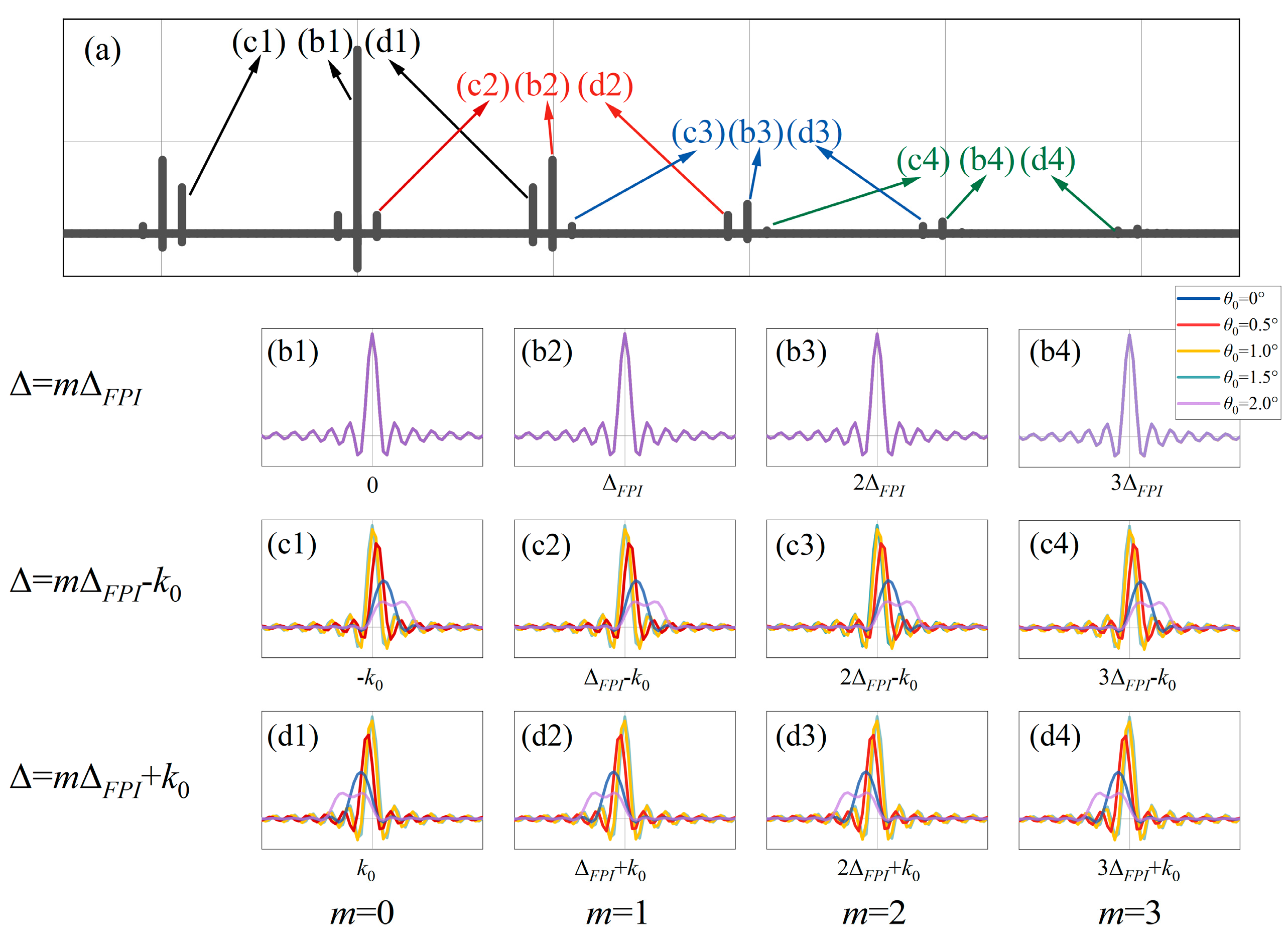
3.2.1. Collimation Error

In practical implementations, the beam exiting the collimation system from an object point exhibits non-ideal collimation with a finite divergence angle. As illustrated in Figure 9, rays with different divergence angles θ generate distinct OPDs in both the FTIS and FPI systems. Assuming uniform intensity distribution across the divergence angle range 2θ₀, the interference intensity of monochromatic light entering the FTIS can be expressed as follows:

$$\begin{array}{ll}{I}_{1-dive}\left(\nu ,\Delta \right)& ={\displaystyle {\int }_0^{2\pi }d\psi {\displaystyle {\int }_0^{{\theta }_0}B\left(\nu \right)\cos \left(2\pi v\Delta \cos \theta \right)\sin \theta d\theta }}/{\displaystyle {\int }_0^{2\pi }d\psi {\displaystyle {\int }_0^{{\theta }_0}\sin \theta d\theta }}\\ & =B\left(\nu \right)\cos \left[2\pi \Delta v\left(1-{\displaystyle \frac{1-\cos {\theta }_0}{2}}\right)\right]\sin \mathrm{c}\left[\Delta v\left(1-\cos {\theta }_0\right)\right]\end{array}.$$

(20)

Under ideal conditions, the interferometric spectrum produced using FTIS is a standard cosine function. Under the influence of the divergence angle, the FTIS two-beam interference introduces a modulation function sinc[νΔ(1 − cosθ₀)] and a wavenumber shift factor (1 − cosθ₀)/2. The effect on the double-beam interferometric spectrum is shown in Figure 10. In Figure 10, with a divergence angle of 1° and OPD values of Δ = 1, 2, and 3 mm, the interferometric spectrum under this error is compared with the ideal case. It can be seen that the divergence angle causes both a reduction in interference intensity and a drift in the wavenumber of the interferometric spectrum. As the OPD increases, the interference intensity at the same wavenumber position decreases, while the wavenumber drift remains unchanged. For the same OPD, as the wavenumber increases, the interference intensity decreases according to the modulation function sinc[νΔ(1 − cosθ₀)], and the periodic frequency of the double-beam interferogram is reduced due to the presence of the wavenumber drift factor.

The maximum incident light divergence angle corresponding to the spectral resolution limit of a conventional FTIS is given by the following:

$${\theta }_0=\sqrt{{\lambda }_{\min }/L}.$$

(21)

The total interference intensity I₁ is

$$\begin{array}{ll}{I}_{1-dive}\left(\Delta \right)& ={\displaystyle {\int }_0^{2\pi }d\psi {\displaystyle {\int }_0^{{\theta }_0}{I}_0\left(\Delta \cos \theta \right)\sin \theta d\theta }}/{\displaystyle {\int }_0^{2\pi }d\psi {\displaystyle {\int }_0^{{\theta }_0}\sin \theta d\theta }}\\ & ={\displaystyle {\int }_{\cos {\theta }_0}^1{I}_0\left(\Delta u\right)du}/\left(1-\cos {\theta }_0\right)\\ & =I_{0-dive}\left(\Delta \right)\end{array}.$$

(22)

The FPI is also affected by the divergence angle, and the incident angle of the same light beam is identical for both FTIS and FPI. The interferogram I₂ is given by the following:

$$\begin{array}{ll}{I}_{2-dive}\left(\Delta \right)& ={\displaystyle {\int }_0^{2\pi }d\psi {\displaystyle {\int }_0^{{\theta }_0}{I}_0\left(\Delta \cos \theta \right)\ast FT\left[a_0+{\displaystyle \sum _{m=1}^{\infty }2a_m\cos \left(m\cdot 2\pi \nu {\Delta }_{FPI}\cos \theta \right)}\right]\sin \theta d\theta }}/{\displaystyle {\int }_0^{2\pi }d\psi {\displaystyle {\int }_0^{{\omega }_0}\sin \theta d\theta }}\\ & =I_{0-dive}\left(\Delta \right)\ast \left[a_0\delta \left(\Delta \right)+{\displaystyle \sum _{m=1}^{\infty }{a}_m\delta \left(\Delta \pm m{\Delta }_{FPI}\right)}\right]\\ & =a_0{I}_{0-dive}\left(\Delta \right)+{\displaystyle \sum _{m=1}^{\infty }{a}_m{I}_{0-dive}\left[\left(\Delta \pm m{\Delta }_{FPI}\right)\right]}\end{array}.$$

(23)

Compared to Equation (6), I₀(Δ) in this equation becomes I_0-dive(Δ) = ∫I₀(Δu)du/(1 − cosθ₀). The frequency-shifted component response function a_mδ(Δ ± mΔ_FPI) remains unchanged, and the linear relationship formed by the FPI does not cause any additional effects. Therefore, the target in Equation (8) also changes from I₀(Δ) to I_0-dive(Δ), while the establishment and solution of the linear equation system remain unaffected. This indicates that the large optical path difference interferogram I₀(Δ) obtained using MJI-HI and the interferogram obtained using FTIS with the same maximum OPD are affected by the divergence angle in the same way. Therefore, the effect of the divergence angle on the MJI-HI with double super-resolution is the same as that on the FTIS with a maximum OPD of 2L. According to Equation (21), the maximum divergence angle for FTIS can be used to derive the maximum divergence angle for MJI-HI as θ₀ = (λ_min/2L) ^1/2.

3.2.2. Beam Splitter Spectral Error

In an ideal FTIS beam splitter, the reflectivity and transmissivity would maintain constant 50% values across all wavenumbers. However, in practical implementations, the reflectivity exhibits wavenumber-dependent variations, which can be modeled as R_FTIS(ν) = 0.5 + δR_FTIS(ν), with the corresponding transmissivity given by T_FTIS(ν) = 1 − R_FTIS(ν), under the assumption of negligible thin-film absorption losses. By incorporating Equation (2) and neglecting the DC component, the interferogram I₁(Δ) can be expressed as follows:

$$\begin{array}{ll}{I}_{1-BS}\left(\Delta \right)& ={\displaystyle \int \left[1-4\delta R_{FTIS}{\left(\nu \right)}^2\right]B\left(\nu \right)}\cos \left(2\pi \nu \Delta \right)d\nu \\ & =FT\left\{\left[1-4\delta R_{FTIS}{\left(\nu \right)}^2\right]B\left(\nu \right)\right\}=I_{0-BS}\left(\Delta \right)\end{array}.$$

(24)

A spectral reflectivity deviation in the beam splitter effectively modifies the incident spectrum to B(ν)[1 − 4δR_FTIS(ν)²]. This perturbation introduces a convolutional distortion in I_1-BS compared to the theoretical interferogram I₀, resulting in a beam-splitter-degraded signal denoted as I_0-BS.

The interferogram I₂ is

$$\begin{array}{ll}{I}_{2-BS}\left(\Delta \right)& ={\displaystyle \int \left[1-4\delta R_{FTIS}{\left(\nu \right)}^2\right]B\left(\nu \right)}{T}_{FPI}\left(\nu \right)\cos \left(2\pi \nu \Delta \right)d\nu \\ & =I_{0-BS}\left(\Delta \right)\ast \left[a_0\delta \left(\Delta \right)+{\displaystyle \sum _{m=1}^{\infty }{a}_m\delta \left(\Delta \pm m\cdot {\Delta }_{FPI}\right)}\right]\end{array}.$$

(25)

The linear relationships between I_1-BS, I_2-BS, and I_0-BS remain fundamentally unchanged, ensuring the inversion computation remains unaffected by these perturbations. The final calculated spectrum corresponds to the modulated spectral signal B(ν)[1 − 4δR_FTIS(ν)²].

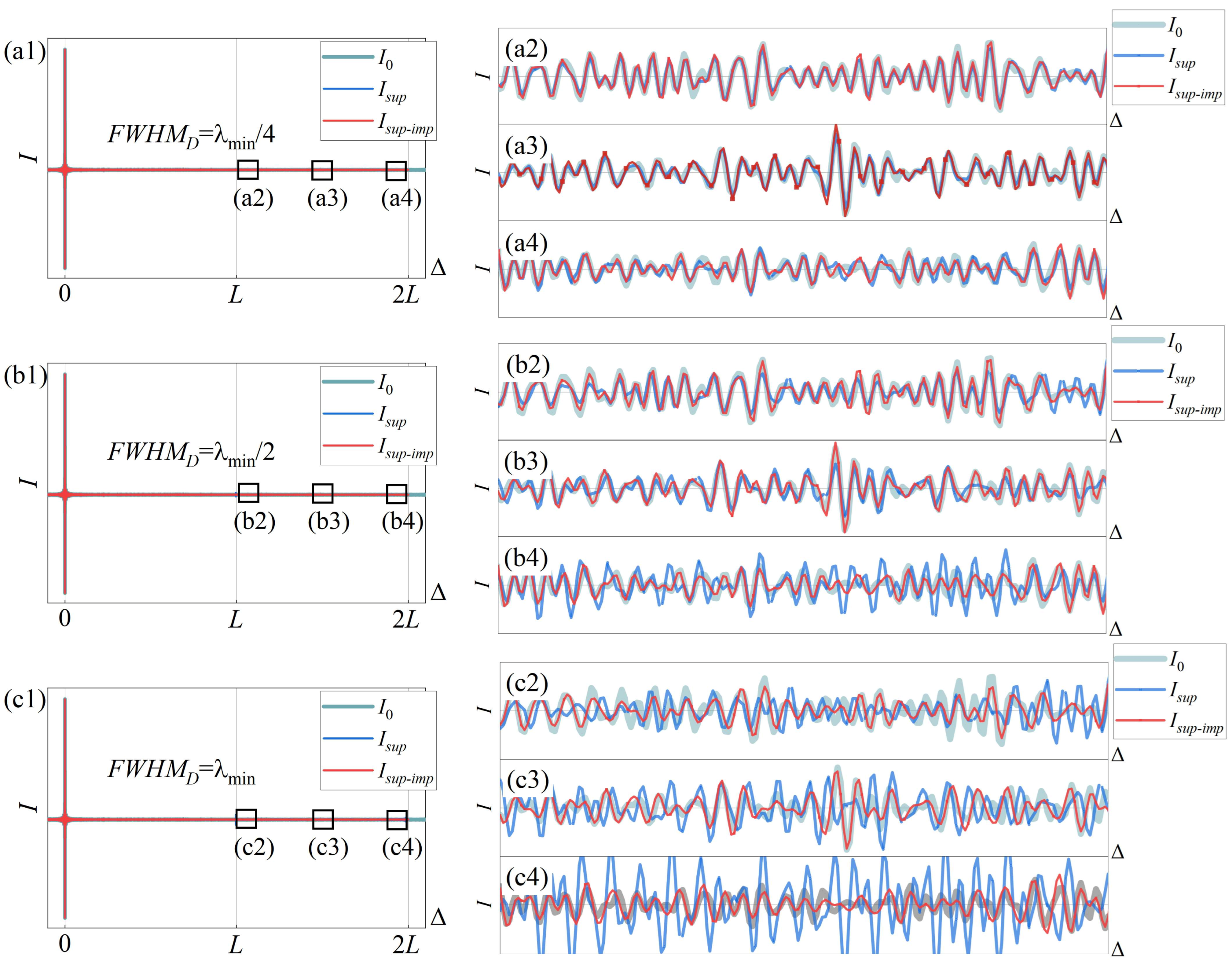
3.2.3. Mirror Tilt Error

In FTIS, optical components such as the fixed mirror, moving mirror, and beam splitter may deviate from their ideal positions due to alignment errors or external vibrations, leading to tilt and other issues. The two coherent parallel beams exiting the interferometer exhibit a wavefront tilt with an angle of 2β_FTIS. This tilt causes variations in the OPD at different positions within the aperture. When the aperture is circular, the normalized distribution of the OPD error is given by the following:

$$g_{FTIS}\left(\sigma \Delta \right)={\displaystyle \frac{1}{\pi {\beta }_{FTIS}{r}_0}}\sqrt{1-{\left(\sigma \Delta /2{\beta }_{FTIS}{r}_0\right)}^2}.$$

(26)

According to Equation (26), the FWHM of g_FTIS(σΔ) is given by FWHM_tilt = $2\sqrt{3}$β_FTISr₀. I₁ can be expressed as follows:

$$\begin{array}{ll}{I}_{1-tilt}\left(\Delta \right)& ={\displaystyle \int d\nu }{\displaystyle {\int }_{-{\beta }_{FTIS}{r}_0}^{{\beta }_{FTIS}{r}_0}B\left(\nu \right)\cos \left[2\pi \nu \left(\Delta +\sigma \Delta \right)\right]g_{FTIS}\left(\sigma \Delta \right)d(\sigma \Delta )}\\ & ={\displaystyle \int \left[B\left(\nu \right)\frac{2J_1\left(2\pi \nu 2r_0{\beta }_{FTIS}\right)}{2\pi \nu 2r_0{\beta }_{FTIS}}\right]\cos \left(2\pi \nu \Delta \right)d\nu }\end{array}.$$

(27)

The Bessel function forms the modulation function, and the higher the wavenumber, the faster the modulation depth decreases. This error does not affect the subsequent FPI, meaning T_FPI(ν) remains unchanged. Similarly, I₂ can be expressed as follows:

$$\begin{array}{ll}{I}_{2-tilt}\left(\nu \right)& ={\displaystyle \int d\nu }{\displaystyle {\int }_{-{\beta }_{FTIS}{r}_0}^{{\beta }_{FTIS}{r}_0}B\left(\nu \right)T_{FPI}\left(\nu \right)\cos \left[2\pi \nu \left(\Delta +\sigma \Delta \right)\right]g_{FTIS}\left(\sigma \Delta \right)d(\sigma \Delta )}\\ & ={\displaystyle \int \left[B\left(\nu \right)T_{FPI}\left(\nu \right)\frac{2J_1\left(2\nu r_0{\beta }_{FTIS}\right)}{2\pi \nu r_0{\beta }_{FTIS}}\right]\cos \left(2\pi \nu \Delta \right)d\nu }\end{array}.$$

(28)

The two interferograms can also be expressed in an integral form as follows:

$$\left\{\begin{array}{l}{I}_{1-tilt}\left(\Delta \right)={\displaystyle {\int }_{-2{\beta }_{FTIS}{r}_0}^{2{\beta }_{FTIS}{r}_0}{I}_0\left(\Delta +\sigma \Delta \right)g_{FTIS}\left(\sigma \Delta \right)d\sigma \Delta }\\ I_{2-tilt}\left(\Delta \right)={\displaystyle {\int }_{-2{\beta }_{FTIS}{r}_0}^{2{\beta }_{FTIS}{r}_0}{I}_0\left(\Delta +\sigma \Delta \right)\ast FT\left[T_{FPI}\left(\nu \right)\right]g_{FTIS}\left(\sigma \Delta \right)d\sigma \Delta }\end{array}\right..$$

(29)

In FTIS, the moving mirror’s positional stability during scanning is critical for maintaining interferometric accuracy. As the moving mirror translates, random tilt angles β_FTIS may arise due to mechanical imperfections, vibrations, or control system limitations. These tilts introduce spatially varying OPDs across the beam aperture. The g_FTIS(σΔ) changes with Δ. Consequently, the acquired interferograms I₁ and I₂ deviate from their idealized forms, manifesting as position-dependent phase noise that scales with β_FTIS.

For the fixed optical components, such as mirrors in SMFTIS and TSMFTIS, or stationary components, like the fixed mirror or beam splitter in FTIS, the tilt angles they introduce are fixed. Consequently, the OPD error distribution g_FTIS(σΔ) becomes a stationary function, allowing the interferogram to be expressed in a convolution form:

$$\left\{\begin{array}{ll}{I}_{1-tilt}\left(\Delta \right)& =I_0\left(\Delta \right)\ast g_{FTIS}\left(\Delta \right)\\ & =I_{0-tilt}\left(\Delta \right)\\ I_{2-tilt}\left(\Delta \right)& =I_0\left(\Delta \right)\ast g_{FTIS}\left(\Delta \right)\ast FT\left[T_{FPI}\left(\nu \right)\right]\\ & =I_{0-tilt}\left(\Delta \right)\ast \left[a_0\delta \left(\Delta \right)+{\displaystyle \sum _{m=1}^{\infty }{a}_m\delta \left(\Delta \pm m\cdot {\Delta }_{FPI}\right)}\right]\end{array}\right..$$

(30)

Both I_1-tilt and I_2-tilt maintain linear relationships with I_0-tilt. The response function a_mδ(Δ ± mΔ_FPI) remains unchanged, and the fixed-tilt-induced errors do not affect the core interferogram inversion algorithm. The reconstructed interferogram I₀ converges to I_0-tilt, demonstrating equivalence to interferograms acquired by an FTIS system with identical tilt errors.

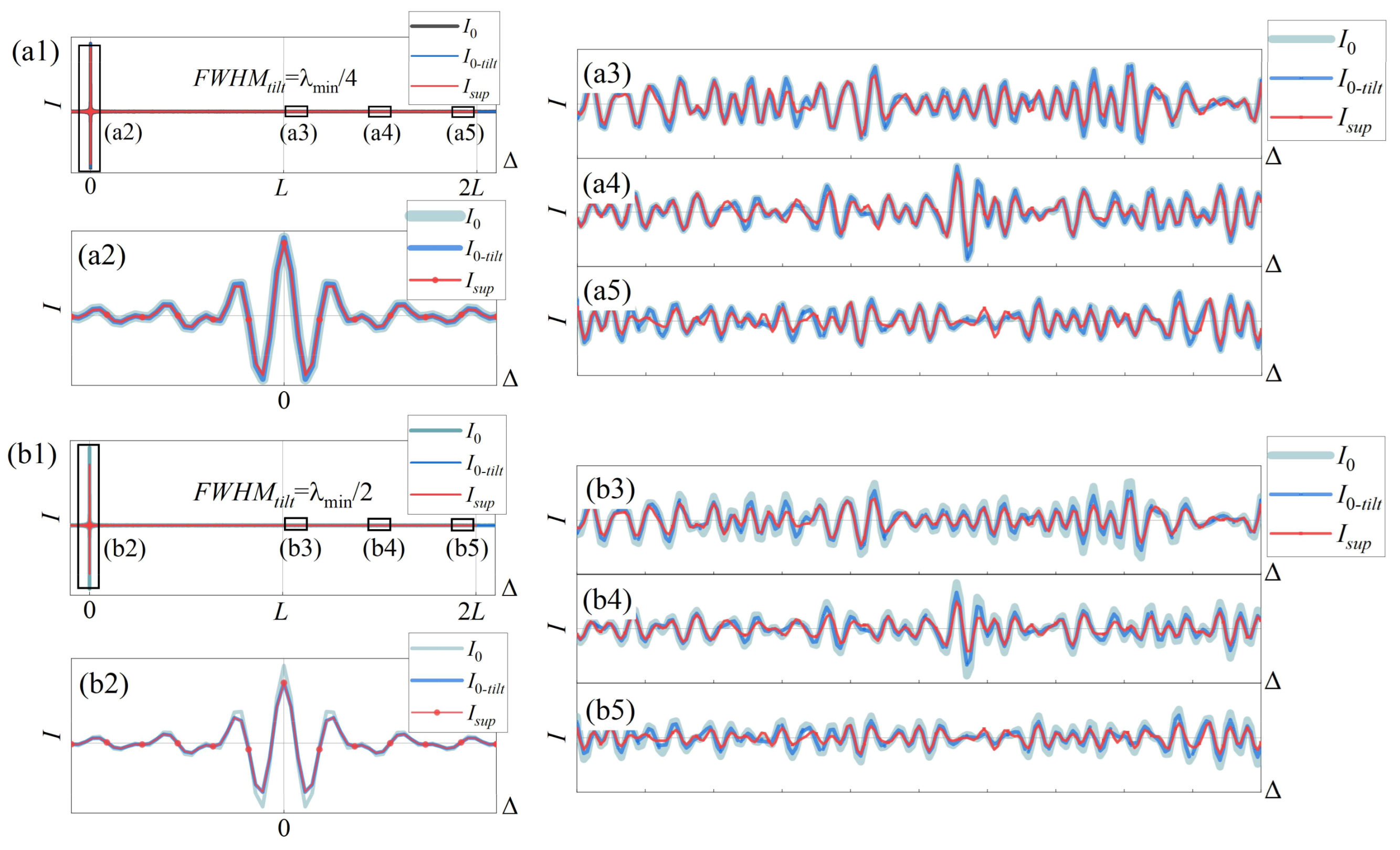
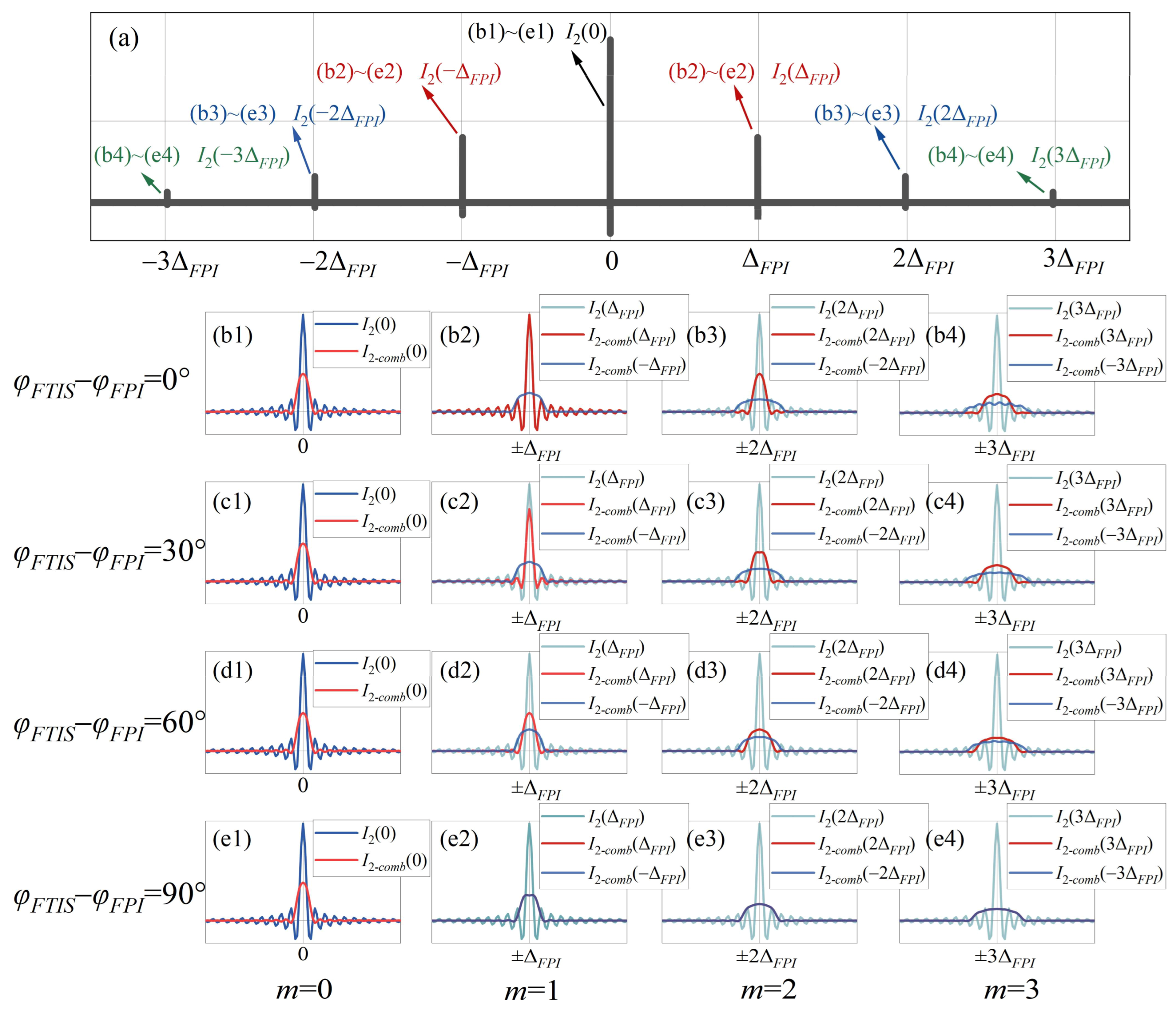
3.2.4. The Combined Error of FPI Non-Parallelism and FTIS Mirror Tilt Error

Non-parallelism errors in the FPI and tilt errors in the FTIS both induce wavefront angles between the coherent beams, where tilt errors in the FTIS manifest as a convolution of I₀(Δ) with g_FTIS(σΔ), while non-parallelism errors in the FPI result in the convolution of each frequency-shifted component a_mI₀(Δ ± Δ_FPI) with g_m(σΔ). Since both the OPD errors in the FTIS and cavity length errors in the FPI are spatially dependent on the beam’s position within the aperture, the combined effects of these errors cannot be linearly superimposed when analyzing the system.

Assuming a circular clear aperture, a polar coordinate system (r,φ) can be established to represent points within the aperture. As shown in Figure 11, let the FTIS be tilted along the φ_FTIS direction with a wavefront tilt angle 2β_FTIS and the FPI be tilted along the φ_FPI direction with a wavefront tilt angle 2β_FPI. For a point (r,φ), the OPD error introduced by the FTIS is σΔ = 2rβ_FTIScos(φ − φ_FTIS), while the cavity length error from the FPI is σΔ_FPI = 2rβ_FPIcos(φ − φ_FPI). Consequently, the monochromatic interference intensity of the interferogram I₂ can be expressed as follows:

$$\left\{\begin{array}{cc}\hfill I_{2-comb}\left(v,\Delta \right)& ={\displaystyle {\int }_0^{r_0}{\displaystyle {\int }_0^{2\pi }rB\left(\nu \right)\cos {\delta }_{FTIS}}}\left\{a_0+{\displaystyle \sum _{m=1}^{\infty }2a_m\cos m{\delta }_{FPI}}\right\}d\phi dr/\left(\pi r_0^2\right)\hfill \\ & ={\displaystyle {\int }_0^{r_0}{\displaystyle {\int }_0^{2\pi }{a}_{0}rB\left(\nu \right)\cos {\delta }_{FTIS}}}+rB\left(\nu \right){\displaystyle \sum _{m=1}^{\infty }{a}_m\left[\cos \left({\delta }_{FTIS}+m{\delta }_{FPI}\right)+\cos \left({\delta }_{FTIS}-m{\delta }_{FPI}\right)\right]}d\phi dr/\left(\pi r_0^2\right)\hfill \\ \hfill {\delta }_{FTIS}& =2\pi \nu \left[\Delta +2r{\beta }_{FTIS}\cos \left(\phi -{\phi }_{FTIS}\right)\right]\hfill \\ \hfill {\delta }_{FPI}& =2\pi \nu \left[{\Delta }_{FPI}+2r{\beta }_{FPI}\cos \left(\phi -{\phi }_{FPI}\right)\right]\hfill \end{array}\right..$$

(31)

In the equation, δ_FTIS represents the interference phase of the FTIS, and δ_FPI denotes the interference phase of the FPI. This expression comprises three components: the DC component of I₂ is given by β₀rB(ν)cosδ_FTIS, while the m-th and −m-th order frequency-shifted components correspond to β_mrB(ν)cos(δ_FTIS− − mδ_FPI) and β_mrB(ν)cos(δ_FTIS + mδ_FPI), respectively. Substituting the phase terms and simplifying yields the final form of the interferogram:

$$\left\{\begin{array}{cc}\hfill {\delta }_{FTIS}-m{\delta }_{FPI}& =2\pi v\left[\left(\Delta -m{\Delta }_{FPI}\right)+2r{\beta }_m\cos \left(\phi -{\phi }_m\right)\right]\hfill \\ \hfill {\delta }_{FTIS}+m{\delta }_{FPI}& =2\pi v\left[\left(\Delta +m{\Delta }_{FPI}\right)+2r{\beta }_{-m}\cos \left(\phi -{\phi }_{-m}\right)\right]\hfill \\ \hfill {\beta }_m& =\sqrt{{\beta }_{FTIS}^2+m^2{\beta }_{FPI}^2-2m{\beta }_{FTIS}{\beta }_{FPI}\cos \left({\phi }_{FTIS}-{\phi }_{FPI}\right)}\hfill \\ \hfill {\beta }_{-m}& =\sqrt{{\beta }_{FTIS}^2+m^2{\beta }_{FPI}^2+2m{\beta }_{FTIS}{\beta }_{FPI}\cos \left({\phi }_{FTIS}-{\phi }_{FPI}\right)}\hfill \\ \hfill {\phi }_m& =\arctan \left[\left({\beta }_{FTIS}\sin {\phi }_{FTIS}-m{\beta }_{FPI}\sin {\phi }_{FPI}\right)/\left({\beta }_{FTIS}\cos {\phi }_{FTIS}-m{\beta }_{FPI}\cos {\phi }_{FPI}\right)\right]\hfill \\ \hfill {\phi }_{-m}& =\arctan \left[\left({\beta }_{FTIS}\sin {\phi }_{FTIS}+m{\beta }_{FPI}\sin {\phi }_{FPI}\right)/\left({\beta }_{FTIS}\cos {\phi }_{FTIS}+m{\beta }_{FPI}\cos {\phi }_{FPI}\right)\right]\hfill \end{array}\right..$$

(32)

Therefore, for the m-th order frequency-shifted component, the combined errors from the FTIS and FPI can be equivalently modeled by generating a new effective tilt angle β_m oriented at φ_m. The same is true for the −m-th order frequency-shifted component. The relationships between β_m, φ_m, and the FTIS/FPI parameters are illustrated in Figure 12. In polar coordinates, the FTIS tilt error is represented as the vector ${\overrightarrow{x}}_{FTIS}$= (β_FTIS,φ_FTIS), while the non-parallelism error of the FPI’s m-th order frequency-shifted component is expressed as ${\overrightarrow{x}}_{FPI}$ = (mβ_FPI,φ_FPI). The equivalent tilt angle is then derived through vector summation in polar coordinates:

$$\left\{\begin{array}{c}\left({\beta }_m,{\phi }_m\right)={\overrightarrow{x}}_{FTIS}-{\overrightarrow{x}}_{FPI}\\ \left({\beta }_{-m},{\phi }_{-m}\right)={\overrightarrow{x}}_{FTIS}+{\overrightarrow{x}}_{FPI}\end{array}.\right.$$

(33)

Only when the tilt direction of FTIS is perpendicular to that of FPI, i.e., |φ_FTIS-φ_FPI| = π/2, the tilt angles β_m and β_−m are equal.

Substituting Equation (32) into Equation (31) gives the following:

$$\begin{array}{ll}{I}_{2-comb}(v,\Delta )& =a_{0}B(v){\displaystyle \frac{2J_1\left(2\pi v2r_0{\beta }_{FTLS}\right)}{2\pi v2r_0{\beta }_{FTIS}}}\cos (2\pi v\Delta )\\ & +{\displaystyle \sum _{m=1}^{\infty }}{a}_{m}B(v)\left\{{\displaystyle \frac{2J_1\left(2\pi v2r_0{\beta }_m\right)}{2\pi v2r_0{\beta }_m}}\cos \left[2\pi v\left(\Delta -m{\Delta }_{FPI}\right)\right]+{\displaystyle \frac{2J_1\left(2\pi v2r_0{\beta }_{-m}\right)}{2\pi v2r_0{\beta }_{-m}}}\cos \left[2\pi v\left(\Delta +m{\Delta }_{FPI}\right)\right]\right\}\end{array}$$

(34)

The total interference light intensity is

$$\left\{\begin{array}{ll}{I}_{2-comb}(\Delta )& =I_0(\Delta )\mathrm{*}\left\{a_0\delta (\Delta )\mathrm{*}{g}_{0-comb}(\Delta )+\sum _{m=1}^{\mathrm{\infty }}{a}_m\left[\delta \left(\Delta -m{\Delta }_{FPI}\right)\mathrm{*}{g}_{m-comb}(\Delta )+\delta \left(\Delta +m{\Delta }_{FPI}\right)\mathrm{*}{g}_{-m-comb}(\Delta )\right]\right\}\\ & =a_0{I}_0(\Delta )\mathrm{*}{g}_{\mathrm{egu} ,0}(\Delta )+\sum _{m=1}^{\mathrm{\infty }}{a}_m\left[I_0\left(\Delta -m{\Delta }_{FPI}\right)\mathrm{*}{g}_{m-comb}(\Delta )+I_0\left(\Delta +m{\Delta }_{FPI}\right)\mathrm{*}{g}_{-m-comb}(\Delta )\right] \\ g_{m-comb}(\Delta )& ={\displaystyle \frac{1}{\pi {\beta }_m{r}_0}}\sqrt{1-{\left(\Delta /2{\beta }_m{r}_0\right)}^2}\\ g_{-m-comb}(\Delta )& ={\displaystyle \frac{1}{\pi {\beta }_{-m}{r}_0}}\sqrt{1-{\left(\Delta /2{\beta }_{-m}{r}_0\right)}^2}\end{array}\right.$$

(35)

The normalized OPD error function for the m-th order, g_m-comb(Δ), is determined by the equivalent tilt angle β_m at each harmonic order m. Compared to Equation (6), the interferogram I₂ can be regarded as having a DC component and frequency-shifted components, each with different tilt angles β_m. The response function a_mδ(Δ − mΔ_FPI) convolves with g_m-comb(Δ), resulting in broadening. Consequently, when both error types coexist, the linear relationship between I_2-comb and I₀ is disrupted, and I_2-comb also loses its inherent symmetry. Such errors may significantly impact the MJI-HI system; thus, these errors must be minimized during system design and alignment to ensure their effects remain negligible.

4. Results and Discussion

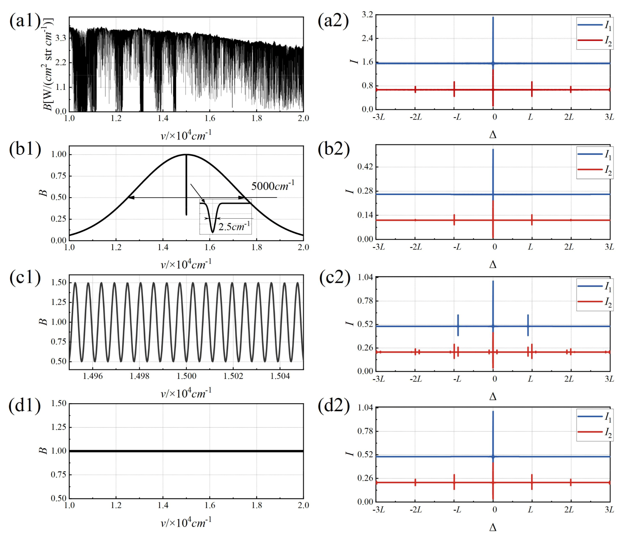
4.1. Error Analysis Simulation Experiment Conditions

We validate and discuss the above error analysis through the simulation experiments of MJI-HI with twofold spectral super-resolution. The main simulation conditions are listed in

Table 1. Simulation experiment conditions.

Simulation Conditions	Parameters
Spectral range	1 × 104~2 × 104 cm−1
Maximum OPD of FTIS	L = 2 mm
Spectral resolution of FTIS	Δν = 1/(2L) = 2.5 cm−1
FPI spacing distance	d = 0.995 mm
Reflectivity of FPI	R0 = 40%

.

The simulation experiments use four different input spectra, and the corresponding input spectra and interferograms are shown in Figure 13, where I₁ represents the interferogram in the optical path without an FPI, and I₂ represents the interferogram in the optical path with an FPI.

Figure 13(a1) shows the atmospheric spectrum calculated based on the HITRAN database, which is used to simulate actual target spectral detection [35]. Figure 13(a2) presents the corresponding interferograms I₁ and I₂, where, due to the effect of the FPI, I₂ exhibits multiple interference peaks at Δ = mΔ_FPI.

The input spectrum in Figure 13(b1) is obtained by subtracting two Gaussian functions with FWHM of 5000 and 2.5 cm⁻¹, where the Gaussian function at 5000 cm⁻¹ represents the low-frequency information of the spectrum, and the Gaussian function at 2.5 cm⁻¹ represents the high-frequency information. Figure 13(b2) shows the corresponding interferogram.

Figure 13(c1) represents an input spectrum modeled as a cosine function with a periodic frequency of k₀ = 1.8 mm: 1 + cos(2πk₀ν)/2; thus, under ideal conditions, the interferogram I₁ can be expressed as I₁ = δ(Δ)+ δ(Δ − k₀)/4 + δ(Δ + k₀)/4, while I₂ contains delta functions at Δ = mΔ_FPI and Δ = mΔ_FPI ± k₀. Thus, using a cosine function as the input spectrum allows the analysis of optical errors affecting different frequency-shifted components in I₂ at both the central position Δ = mΔ_FPI and the shifted positions Δ = mΔ_FPI ± k₀.

Figure 13(d1) represents an input spectrum of a constant value of 1, and the corresponding interferogram I₂ exhibits delta functions at Δ = mΔ_FPI, enabling the analysis of how optical errors affect the response functions of different frequency-shifted components.

By using different input spectra, the effects of various errors on the response functions of the frequency-shifted components are simulated and analyzed, along with the changes in the final super-resolution interferograms or spectra obtained using MJI-HI.

4.2. Simulation Experiment Results

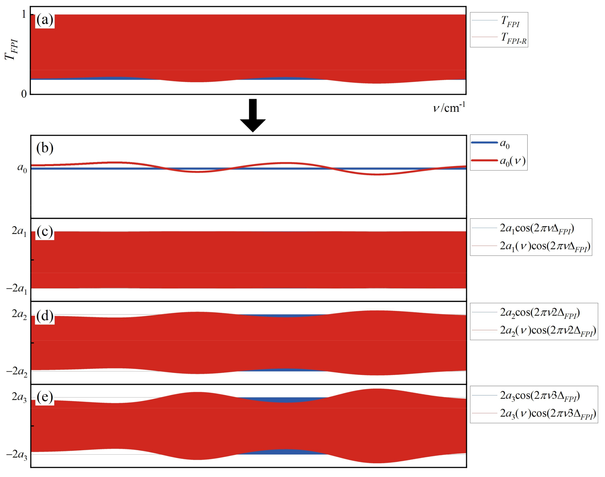
4.2.1. Broadening of the FPI Response

The non-parallelism and non-flatness errors of the FPI both lead to a decrease in multi-beam interference intensity and a broadening of the response function. Using B₀ = 1 as the input spectrum, a simulation analysis of the interferogram I₂ was conducted under different degrees of non-parallelism and non-flatness. According to Equation (17), at this point, I₂(Δ) can be expressed as the sum of the response functions a₀δ(Δ) + a_mδ(Δ ± mΔ_FPI) ∗ Defect_m(Δ), and the results of these response functions are shown in Figure 14. The simulations examined cases where FWHM_para and FWHM_flat were set to 0, λ_min/8(0.0625 μm), λ_min/4(0.125 μm), and λ_min/2(0.25 μm), respectively. When the optical defects of the FPI are zero, its interferogram is consistent with Equation (6), where the response function of each frequency-shifted component, a_mδ(Δ ± mΔ_FPI), is a δ function with energy decreasing stepwise. However, when non-parallelism and non-flatness exist, its interferogram matches Equation (17), and the DC component remains unaffected, while the response functions of higher-order frequency-shifted components undergo convolution with g_m and p_m, becoming a_mδ(Δ ± mΔ_FPI) ∗ Defect_m(Δ). As the order m of the frequency shift increases, the broadening of the frequency-shifted components increases progressively by a factor of m, and their amplitude decreases stepwise to 1/m. Larger optical defects lead to lower interference intensity. The simulation results are consistent with the analysis presented in Section 3.

When the broadening caused by FPI defects is relatively small, its impact can be neglected. Considering both optical defects comprehensively, the full width at half maximum (FWHM_D) of Defect₁ in Equation (17) is λ_min/4(0.125 μm), λ_min/2(0.25 μm), and λ_min (0.5 μm), respectively, with the broadening caused by non-parallelism and non-flatness each accounting for 50%. The interferogram reconstruction is performed using both the improved algorithm from Section 3.1.3 and the unimproved algorithm, and the results are shown in Figure 15. The red curve in the figure represents I_sup-imp, while the blue curve represents I_sup. From the results, it can be observed that when FWHM_D is small, the results of the improved and unimproved algorithms are relatively close. As FWHM_D increases, the error of I_sup also increases, whereas the results of I_sup-imp remain more stable and accurate. By applying the IFT to these interferograms, the super-resolution spectra are obtained, and their errors are calculated based on the following equation:

$$Error(dB)=10\lg \left[{\displaystyle \frac{{\displaystyle \sum {\left[B^{\prime }\left(\nu \right)-B\left(\nu \right)\right]}^2}}{{\displaystyle \sum {\left[B\left(\nu \right)\right]}^2}}}\right].$$

(36)

When FWHM_D is λ_min/4, λ_min/2, and λ_min, the errors of the improved algorithm are −18.70 dB, −18.74 dB, and −18.38 dB, respectively, while the errors of the unimproved algorithm are −18.60 dB, −18.04 dB, and −15.55 dB. The error of the unimproved algorithm increases significantly as non-parallelism increases, whereas the improved algorithm maintains a smaller and nearly constant error. Therefore, the improved algorithm is feasible and effective.

According to the Nyquist sampling theorem, the minimum sampling interval of the interferogram is λ_min/2, which, in this simulation, is 0.25 μm. Based on this, if the FWHM of the OPD error function of the FPI optical defect is smaller than λ_min/4, the broadening effect can be considered negligible. With the current mature FPI manufacturing technology, the non-parallelism tilt angle is typically better than 1″, and the non-flatness is within tens of nanometers, usually meeting this threshold. However, for cases with large broadening caused by special conditions such as large aperture sizes, this issue can be addressed using the improved algorithm.

4.2.2. Mirror Tilt Error of FTIS

According to the analysis in Section 3.2.2, the effect of fixed tilt error is to convolve I₀(Δ) with the optical path error function g_FTIS(Δ). For the interferogram I₂(Δ), this effect can be considered as each frequency-shifted component a_mI₀(Δ ± Δ_FPI) being convolved with g_FTIS(Δ). Therefore, I₁(Δ) and I₂(Δ) still maintain a linear relationship with I₀(Δ) ∗ g(Δ). Using Hitran spectral data as the input spectrum, we simulated and analyzed the MJI-HI spectral super-resolution results for cases where the FWHM of g_FTIS(Δ) is λ_min/4 (0.125 μm) and λ_min/2 (0.25 μm), as shown in Figure 16. Here, I₀ represents the FTIS interferogram without fixed tilt error, I_0-tilt represents the FTIS interferogram with fixed tilt error, and I_sup is the MJI-HI interferogram reconstruction result in the presence of fixed tilt error. The simulation results indicate that since the linear relationship is preserved, the reconstruction results remain highly accurate and conform to the mathematical model of the inversion algorithm. Converting I_0-tilt and I_sup into spectra and computing their errors relative to B₀ using Equation (36), we find that when FWHM_tilt = 0.125 μm, the errors for I_0-tilt and I_sup are −17.85 dB and −17.69 dB, respectively. When FWHM_tilt = 0.25 μm, the errors are −12.10 dB and −11.91 dB, respectively. The decrease in accuracy is due to the reduction in interferogram intensity, leading to spectral energy loss, which requires spectral correction processing. From the interferogram and spectral error comparison between I_sup and I_0-tilt, it can be observed that both are closer to each other than to I₀, indicating that the inversion algorithm produces results equivalent to I₀(Δ) ∗ g(Δ). Therefore, the fixed tilt error requirement for MJI-HI is the same as that for FTIS with the same aperture size, i.e., β_FTIS < 1/(14ν_maxr₀).

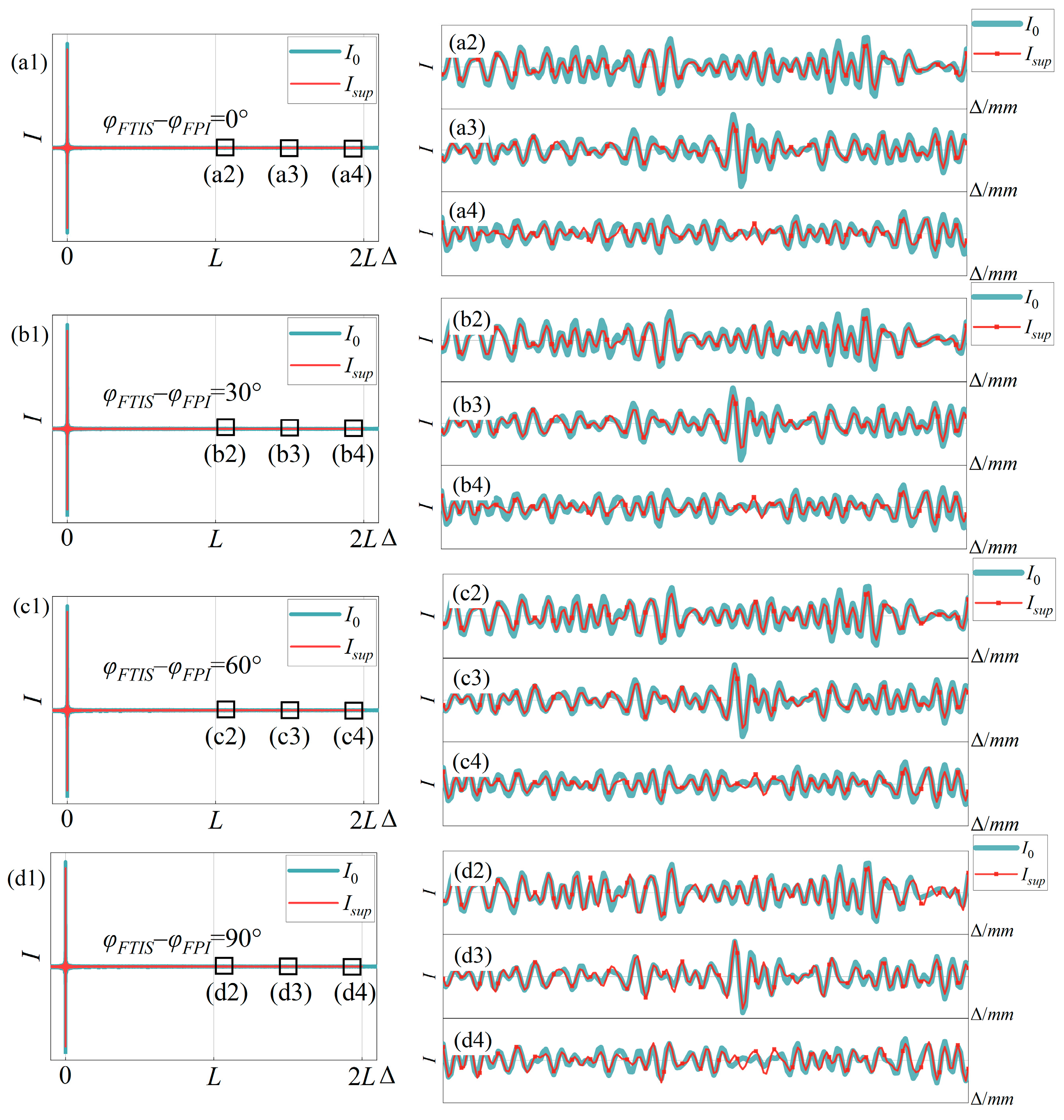
4.2.3. The Combined Error of FPI and FTIS

According to the analysis in Section 3.2.4, when both the FTIS tilt error and the FPI non-parallelism error are present, their combined effect on the interferogram can be equivalently considered as each m-th order frequency-shifted component experiencing a tilt error with an angle β_m. The magnitude of β_m depends on the tilt angles of FTIS (β_FTIS) and FPI (β_FPI), as well as the angle φ_FTIS − φ_FPI between their respective tilt directions. Assuming that the FTIS has a tilt angle of β_FTIS = 1″ and the FPI has a tilt angle of β_FPI= 1″, with tilt direction angles of φ_FTIS − φ_FPI = 0°, 30°, 60°, and 90°, we simulate the interferograms I₂(0), I₂(±Δ_FPI), I₂(±2Δ_FPI), and I₂(±3Δ_FPI) under these tilt error conditions using an input spectrum of B(ν) = 1. Based on Equation (35), under these simulation conditions, the interferograms are given by the following: I_2-comb(0) = a₀δ(Δ) ∗ g_0-comb(Δ), I_2-comb(mΔ_FPI) = a_mδ(Δ − mΔ_FPI) ∗ g_m-comb(Δ), and I_2-comb(−mΔ_FPI) = a_mδ(Δ + mΔ_FPI) ∗ g_−m-comb(Δ), which represent the response functions of each frequency-shifted component. The simulation results are shown in Figure 17, where I₂ (Δ) represents the ideal interferogram without errors, and I_2-comb(mΔ_FPI) and I_2-comb(−mΔ_FPI) are shifted to the same central position for comparison. It can be observed that as m increases, the convolution-broadening effect of g_m-comb(Δ) and g_−m-comb(Δ) on the response functions becomes more pronounced, indicating that β_m increases with m. For the m = 0 order, since β₀ = β_FTIS, the broadening caused by g_0-comb (Δ) remains the same regardless of φ_FTIS − φ_FPI. As shown in Figure 17(d1–d4,e1–e4), for m = 1,2,3, the difference between I_2-comb(mΔ_FPI) and I_2-comb(−mΔ_FPI) is the largest when φ_FTIS − φ_FPI = 0°, and as the angle approaches 90°, I_2-comb(mΔ_FPI) and I_2-comb(−mΔ_FPI) gradually converge. These simulation results are consistent with the analysis presented in Section 3.2.4.

Using the Hitran spectral data from Figure 13(a1,a2) as the input spectrum, the MJI-HI interferogram calculation results under the combined effects of FPI non-parallelism errors and FTIS tilt errors were obtained. We assume the FPI non-parallelism error satisfies FWHM_para= λ_min/4 (0.125 μm), as defined in Equation (13), and the FTIS tilt error satisfies FWHM_tilt = λ_min/4 (0.125 μm). The MJI-HI super-resolution interferogram I_sup calculation results for tilt direction angle differences of φ_FTIS − φ_FPI = 0°, 30°, 60°, and 90° were calculated separately, as shown in Figure 18. The results demonstrate that under these error conditions, the reconstructed I_sup remains largely consistent with I₀, with minor deviations, indicating a limited impact on MJI-HI performance. Converting I_sup to super-resolved spectra and calculating the error relative to B₀ using Equation (36), the errors for φ_FTIS − φ_FPI = 0°, 30°, 60°, and 90° are −17.61 dB, −17.63 dB, −17.65 dB, and −17.61 dB, respectively. These values closely align with the super-resolved spectral error (−17.85 dB) observed in Section 4.2.2 under FTIS tilt error alone (FWHM_tilt = 0.125 μm). This similarity arises because the interferogram I₁, also affected by FTIS tilt errors, becomes I_1-tilt, leading to final results closer to I_0-tilt. The slight precision degradation stems from reduced interference intensity due to FTIS tilt errors, which lowers the spectral energy. These findings confirm that when the FPI and FTIS broadening widths are better than I_0-tilt, the super-resolved spectra maintain high accuracy regardless of the angular offset between tilt directions.

4.2.4. Collimation Error of FTIS

According to the analysis in Section 3.2.1, the effect caused by the divergence angle is that the target interferogram I₀ becomes I_0-dive(Δ) = ∫I₀(Δu)du/(1 − cosθ₀). Therefore, when Δ is small, I_0-dive(Δ) will approach I₀, and when Δ is large, Δu will cause a larger shift. Using the cosine function from Figure 13(c1,c2) as the input spectrum, the interferogram I₂(Δ) will have δ functions at Δ = mΔ_FPI, Δ = mΔ_FPI + k₀, and Δ = mΔ_FPI − k₀. Simulations were conducted with maximum divergence angles θ₀ = 0°,0.5°,1.0°,1.5°, and 2.0°, with the results shown in Figure 19. As shown in Figure 19(b1–b4), the interferograms of I₂(mΔ_FPI) are almost identical for different divergence angles, indicating that the effect on the center of each frequency-shifted component can be ignored. As shown in Figure 19(c1–c4,d1–d4), in the interferogram of I₂(mΔ_FPI ± k₀), the δ functions broaden, and the width increases with the divergence angle. Additionally, the δ functions also shift, with the shift increasing as the divergence angle increases. As the order m increases, the broadening width and central shift remain unchanged. Therefore, the divergence angle affects I_0-dive(Δ), but I₂ and I₁ still maintain a linear relationship, and the inversion algorithm does not introduce additional errors.

Using the Gaussian function from Figure 13(c1,c2) as the input spectrum, the effect of the divergence angle on the super-resolved spectrum is analyzed. Simulations were conducted with the maximum divergence angles of θ₀ = 0°, 1.0°, and 2.0°, with the results shown in Figure 20. The simulation results show that the divergence angle has little effect on the Gaussian function with FWHM = 5000 cm⁻¹, which represents low-frequency information. However, for the Gaussian function with FWHM = 2.5 cm⁻¹, which represents high-frequency information, the divergence angle causes a shift in the center wavenumber and an increase in width. This is consistent with the conclusion from Equation (20), where the divergence angle reduces the coherent intensity, leading to a decrease in spectral resolution, and also produces a wavenumber drift factor (1 − cosθ₀)/2.

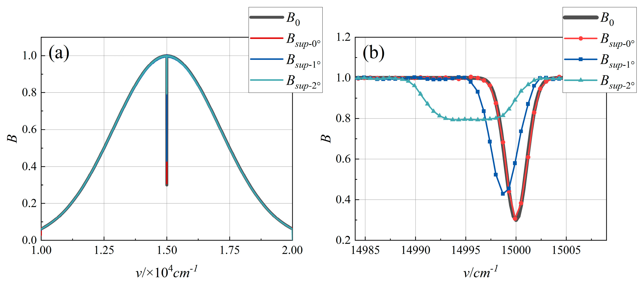
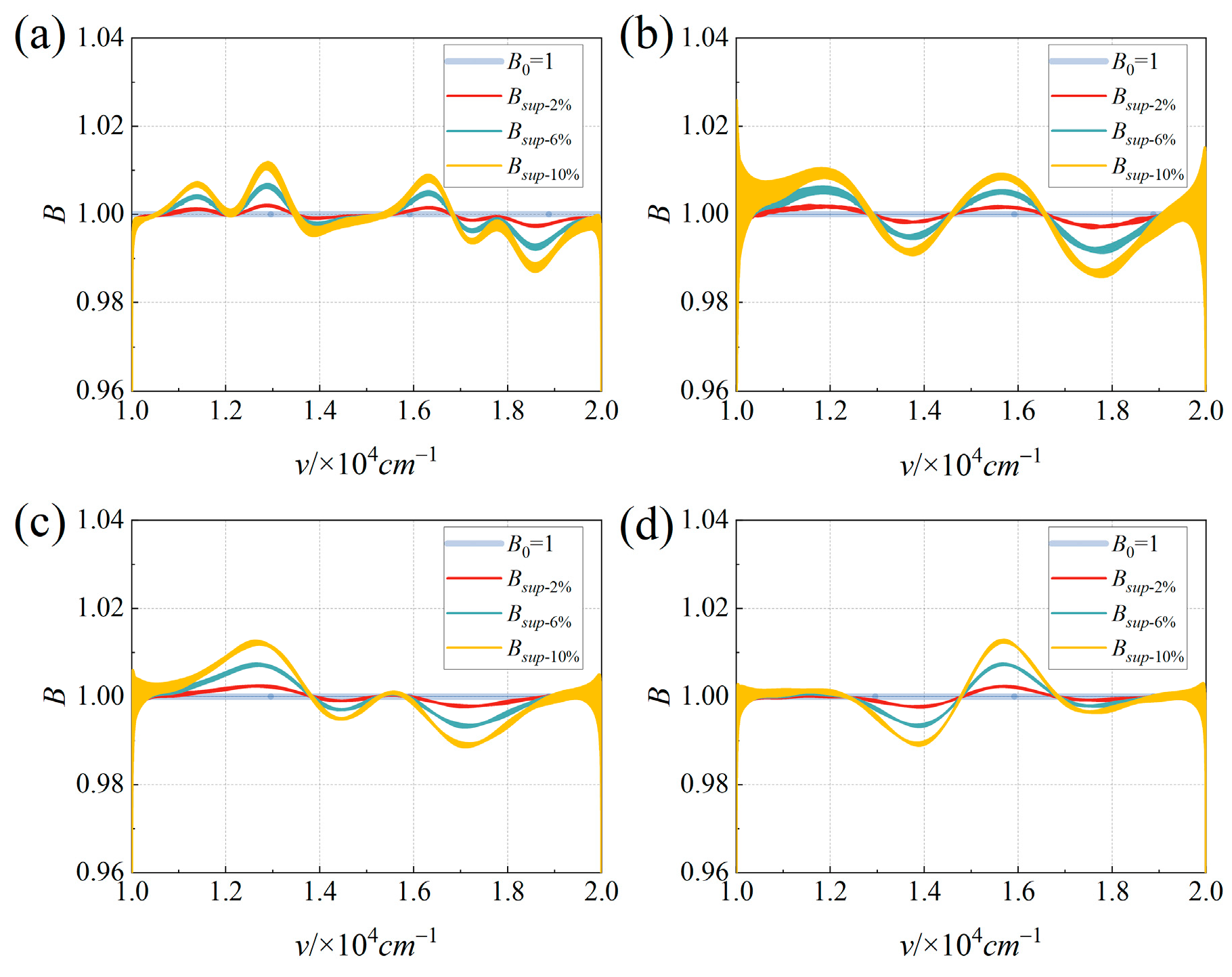
4.2.5. Reflectivity Variation Error of FPI

Based on the analysis in Section 3.1.4, changes in reflectance R cause a change in a_m, which is wavelength-dependent, and the sensitivity of a_m to changes in R varies for different orders of m. Using B₀ = 1 as the input spectrum in Figure 13, the effect of changes in R is analyzed based on I₂. When R is fixed, I₂(Δ) can be expressed as ∑a_mδ(Δ ± mΔ_FPI). When R changes, the difference between [a_m + a′_m${\tilde{R}}_m$(Δ)] ∗ δ(Δ ± mΔ_FPI) and a_mδ(Δ ± mΔ_FPI) allows us to evaluate the effect of reflectance variation on the interference pattern. Assuming an average reflectance of 40%, four smooth curves with different complexities are randomly generated to represent the variations in reflectance. The curves are scaled proportionally so that their maximum–minimum values are set to PV = 2%, 6%, and 10%, which simulate film layer reflectance tolerances of ±1%, ±3%, and ±5%. The simulation results for [a_m + a′_m${\tilde{R}}_m$(Δ)] ∗ δ(Δ ± mΔ_FPI) for m = 0 to 3 are shown in Figure 21. It can be observed that these δ functions remain consistent across different PV values. It can be concluded that changes in reflectance do not affect the linear relationship between I₁ and I₂, and the inversion algorithm remains applicable. For m = 0, 2, 3, slight differences appear at the side lobes of the δ functions as the PV value changes, whereas the δ function for m = 1 remains mostly unchanged. This is because R₀ = 40% is close to the zero point a_1′ of 41.3% in Equation (18), making a₁ less sensitive to changes in reflectance.

Using B₀ = 1 as the input spectrum, the simulation results of the MJI-HI super-resolved spectra for different PV values of the FPI reflectance are shown in Figure 22. It can be observed that the spectrum has become a curve due to the variation in R, and its shape is consistent with the four curves. For the case of a reflectance PV of 10%, the maximum fluctuation in the super-resolved spectrum for the four curves is approximately 0.024 to 0.025, which accounts for 2.4% to 2.5% of B₀, indicating that the impact on the spectrum is relatively small.

Based on the above analysis, the primary errors in the FPI include OPD offset, non-parallelism, surface irregularity, and reflectivity variations. Among these, OPD offset affects the positions of frequency-shifted components but does not disrupt the system’s linear relationship. This error can be calibrated by analyzing interference peaks in the joint interferogram. Non-parallelism and surface irregularity, which are errors of the same type, cause position-dependent optical path differences (OPDs) across the clear aperture. Their impact on the interferogram manifests as a convolution of each frequency-shifted component with the error distribution function, thereby degrading the linear relationship. When these errors are small, their effects can be neglected; however, for larger errors, the error distribution function must be incorporated into the system matrix by replacing the corresponding coefficients with vectorized representations, effectively simulating the convolution’s impact algorithmically. Reflectivity variations have a negligible effect on the linear relationship and can be ignored, as reflectivity tolerances within ±5% remain acceptable for the MJI-HI operation. The resulting super-resolved spectrum may exhibit distortions due to the reflectivity curve, but these can be corrected during spectral radiance calibration.

The primary errors in FTIS include collimation errors, beam splitter reflectivity spectral errors, and mirror tilt errors. These errors do not affect the linear relationship and do not deviate from the fundamental MJI-HI model. However, they introduce certain inaccuracies in the final calculated spectrum. Collimation errors cause wavenumber shifts and reduced spectral resolution, beam splitter errors lead to spectral distortions, and mirror tilt errors result in reduced coherence intensity. Notably, the mirror tilt errors in FTIS may interact with the non-parallelism errors in FPI, introducing an equivalent tilt angle for each frequency-shifted component in I₂. This interaction not only disrupts the linear relationship in MJI-HI but also causes the interferogram I₂ to lose symmetry. Through simulation analysis, it has been determined that MJI-HI maintains high inversion accuracy when the FWHM of the FTIS tilt error broadening function and the FPI non-parallelism error broadening function are both less than λ_min/4. Under these conditions, the effects of these errors can be neglected.

5. Conclusions

This study conducts a comprehensive optical error analysis of the spectral super-resolution technology based on the integration of a Fabry–Pérot interferometer (FPI) and Fourier-transform imaging spectroscopy (FTIS), referred to as the multi-component joint interferometric imaging spectrometer (MJI-HI). The foundational principle of MJI-HI is to generate multiple frequency-shifted components on the interferogram through the periodic modulation of the spectrum by the FPI and obtain a joint interferogram via linear superposition. The inversion algorithm establishes a system of linear equations based on the linear relationship between the joint interferogram and the original interferogram, enabling the recovery of high-frequency information carried by these frequency-shifted components that exceed the maximum OPD of the FTIS. However, the presence of certain optical errors disrupts this linear relationship, leading to reduced accuracy in interferogram reconstruction.

The primary errors in the FPI include optical path errors, non-parallelism errors, surface irregularity errors, and reflectivity variation errors. Based on the analysis results, an OPD calibration algorithm is proposed, and an improved inversion algorithm is developed to address the convolutional errors caused by non-parallelism and surface irregularities in the interferogram. For the FTIS, the main errors include collimation errors, mirror tilt errors, and beam splitter reflectivity variation errors. Based on the analysis results, these errors do not affect the linear relationship of MJI-HI but may lead to spectral distortion, wavelength shift, and energy reduction in the super-resolved spectra caused by diminished interference intensity. Among these, the tilt errors in the FTIS and the non-parallelism errors in the FPI exhibit mutual influence. This paper provides a detailed analysis of these interactions and establishes tolerance thresholds through simulation experiments, demonstrating that the impact of these errors on MJI-HI is negligible within the tolerance limits.

This study comprehensively summarizes the critical technical aspects of MJI-HI, validates the analysis through simulation experiments, and verifies the proposed improved algorithms. It offers detailed theoretical guidance for subsequent experimental development and research on MJI-HI, while also serving as an important theoretical reference for other optical technologies combining FPI and FTIS.

References

1. Zhang, W.; Wen, D.; Song, Z.; Wei, X.; Liu, G.; Li, Z. High Resolution and Fast Processing of Spectral Reconstruction in Fourier Transform Imaging Spectroscopy. Sensors 2018, 18, 4159. [Google Scholar] [CrossRef] [PubMed]
2. Horrocks, T.; Wedge, D.; Hackman, N.; Green, T.; Holden, E.J. Automated Geological Logging from FTIR Reflectance Spectra Utilising Geochemical and Historical Logging Constraints. Ore Geol. Rev. 2024, 168, 106004. [Google Scholar] [CrossRef]
3. Zhu, Q.; Wang, W.; Shan, C.; Xie, Y.; Zeng, X.; Wu, P.; Liang, B.; Liu, C. Effects of Biomass Burning on CO, HCN, C2H6, C2H2 and H2CO during Long-Term FTIR Measurements in Hefei, China. Opt. Express 2024, 32, 8343. [Google Scholar] [CrossRef]
4. Wiercik, P.; Kuśnierz, M.; Kabsch-Korbutowicz, M.; Plucińska, A.; Chrobot, P. Evaluation of Changes in Activated Sludge and Sewage Sludge Quality by FTIR Analysis and Laser Diffraction. Desalin. Water Treat. 2022, 273, 114–125. [Google Scholar] [CrossRef]
5. Cubas Pereira, D.; Pupin, B.; De Simone Borma, L. Influence of Sample Preparation Methods on FTIR Spectra for Taxonomic Identification of Tropical Trees in the Atlantic Forest. Heliyon 2024, 10, e27232. [Google Scholar] [CrossRef]
6. Barragán, R.C.; Castrellon-Uribe, J.; Garcia-Torales, G.; Rodríguez-Rivas, A. IR Characterization of Plant Leaves, Endemic to Semi-Tropical Regions, in Two Senescent States. Appl. Opt. 2020, 59, E126–E133. [Google Scholar] [CrossRef] [PubMed]
7. Suto, H.; Kataoka, F.; Kikuchi, N.; Knuteson, R.O.; Butz, A.; Haun, M.; Buijs, H.; Shiomi, K.; Imai, H.; Kuze, A. Thermal and Near-Infrared Sensor for Carbon Observation Fourier Transform Spectrometer-2 (TANSO-FTS-2) on the Greenhouse Gases Observing SATellite-2 (GOSAT-2) during Its First Year in Orbit. Atmos. Meas. Tech. 2021, 14, 2013–2039. [Google Scholar] [CrossRef]
8. Wei, R.; Zhang, X.; Zhou, J.; Zhou, S. Designs of Multipass Optical Configurations Based on the Use of a Cube Corner Retroreflector in the Interferometer. Appl. Opt. 2011, 50, 1673. [Google Scholar] [CrossRef]
9. Carli, B.; Carlotti, M.; Mencaraglia, F.; Rossi, E. Far-Infrared High-Resolution Fourier Transform Spectrometer. Appl. Opt. 1987, 26, 3818. [Google Scholar] [CrossRef]
10. Ahn, J.; Kim, J.-A.; Kang, C.-S.; Kim, J.-W.; Kim, S. High Resolution Interferometer with Multiple-Pass Optical Configuration. Opt. Express 2009, 17, 21042. [Google Scholar] [CrossRef]
11. Wei, R.Y.; Di, L.M.; Qiao, N.Z.; Chen, S.S. W-shaped common-path interferometer. Appl. Opt. 2020, 59, 10973–10979. [Google Scholar] [CrossRef] [PubMed]
12. Svensson, T.; Bergström, D.; Axelsson, L.; Fridlund, M.; Hallberg, T. Design, calibration and characterization of a low-cost spatial Fourier transform LWIR hyperspectral camera with spatial and temporal scanning modes. In Algorithms and Technologies for Multispectral, Hyperspectral, and Ultraspectral Imagery XXIV; SPIE: Orlando, FL, USA, 2018; pp. 261–275. [Google Scholar]
13. Cai, Q.; Xiangli, B.; Fu, Q.; Qian, L.; Li, Y.; Tan, Z. Conceptual Design of a Rotating Parallel-Mirror-Pair Interferometer. In Selected Papers from Conferences of the Photoelectronic Technology Committee of the Chinese Society of Astronautics: Optical Imaging, Remote Sensing, and Laser-Matter Interaction 2013, Suzhou, China, 20–29 October 2013; Ojeda-Castaneda, J., Han, S., Jia, P., Fang, J., Fan, D., Qian, L., Gu, Y., Yan, X., Eds.; SPIE Digital Library: Bellingham, WA, USA, 2014; p. 91420I. [Google Scholar]
14. Jackson, R.S. Continuous Scanning Interferometers for Mid-Infrared Spectrometry. In Handbook of Vibrational Spectroscopy; Chalmers, J.M., Griffiths, P.R., Eds.; Wiley: Hoboken, NJ, USA, 2001; ISBN 978-0-471-98847-2. [Google Scholar]
15. Châteauneuf, F.; Soucy, M.-A.; Perron, G.; Lévesque, L.; Tanii, J. Reliability Enhancement Activities for the TANSO Interferometer; Strojnik, M., Ed.; SPIE Digital Library: San Diego, CA, USA, 2006; p. 62970M. [Google Scholar]
16. Yu, L.; Li, H.; Li, J.; Li, W. Lossless Compression of Large Aperture Static Imaging Spectrometer Data. Appl. Sci. 2023, 13, 5632. [Google Scholar] [CrossRef]
17. Lucey, P.G.; Akagi, J.; Bingham, A.L.; Hinrichs, J.L.; Knobbe, E.T. A Compact Fourier Transform Imaging Spectrometer Employing a Variable Gap Fabry-Perot Interferometer; Druy, M.A., Crocombe, R.A., Eds.; SPIE Digital Library: Baltimore, MA, USA, 2014; p. 910110. [Google Scholar]
18. Zucco, M.; Pisani, M.; Caricato, V.; Egidi, A. A Hyperspectral Imager Based on a Fabry-Perot Interferometer with Dielectric Mirrors. Opt. Express 2014, 22, 1824. [Google Scholar] [CrossRef] [PubMed]
19. Pisani, M.; Zucco, M.E. Compact Imaging Spectrometer Combining Fourier Transform Spectroscopy with a Fabry-Perot Interferometer. Opt. Express 2009, 17, 8319. [Google Scholar] [CrossRef]
20. Al-Saeed, T.A.; Khalil, D.A. Fourier Transform Spectrometer Based on Fabry–Perot Interferometer. Appl. Opt. 2016, 55, 5322. [Google Scholar] [CrossRef]
21. Swinyard, B.; Ferlet, M. Cascaded Interferometric Imaging Spectrometer. Appl. Opt. 2007, 46, 6381. [Google Scholar] [CrossRef] [PubMed]
22. Yang, Q. Compact Ultrahigh Resolution Interferometric Spectrometer. Opt. Express 2019, 27, 30606. [Google Scholar] [CrossRef]
23. Iwata, T.; Koshoubu, J. Proposal for High-Resolution, Wide-Bandwidth, High-Optical-Throughput Spectroscopic System Using a Fabry-Perot Interferometer. Appl. Spectrosc. 1998, 52, 1008–1013. [Google Scholar] [CrossRef]
24. Yang, Q. Theoretical Analysis of Compact Ultrahigh-Spectral-Resolution Infrared Imaging Spectrometer. Opt. Express 2020, 28, 16616. [Google Scholar] [CrossRef]
25. Zhang, Y.; Liu, Y.; Wang, J.; Tang, Y.; He, P.; Chen, X.; Lv, Q. Joint Interference Imaging Spectral Super-Resolution Technology Based on FPI Modulation. In Proceedings of the Sixth Conference on Frontiers in Optical Imaging and Technology: Novel Imaging Systems, Nanjing, China, 22–24 October 2023; SPIE: Bellingham, WA, USA, 2024; Volume 13155, pp. 350–363. [Google Scholar]
26. Zhang, Y.; Lv, Q.; Tang, Y.; He, P.; Zhu, B.; Sui, X.; Yang, Y.; Bai, Y.; Liu, Y. Super-Resolution Multicomponent Joint-Interferometric Fabry–Perot-Based Technique. Appl. Sci. 2023, 13, 1012. [Google Scholar] [CrossRef]
27. McGill, M.J.; Skinner, W.R.; Irgang, T.D. Analysis Techniques for the Recovery of Winds and Backscatter Coefficients from a Multiple-Channel Incoherent Doppler Lidar. Appl. Opt. 1997, 36, 1253. [Google Scholar] [CrossRef] [PubMed]
28. Ghildiyal, S.; Balasubramaniam, R.; John, J. Effect of Flatness and Parallelism Errors on Fiber Optic Fabry Perot Interferometer of Low to Moderate Finesse and Its Experimental Validation. Opt. Fiber Technol. 2020, 60, 102372. [Google Scholar] [CrossRef]
29. Sloggett, G.J. Fringe Broadening in Fabry-Perot Interferometers. Appl. Opt. 1984, 23, 2427. [Google Scholar] [CrossRef]
30. Fahua, S.; Yiqi, X.; Aiai, Y.; Chenglin, L. Transmission spectral characteristics of F-P interferometer under multi-factors. Infrared Laser Eng. 2015, 44, 1800–1805. [Google Scholar]
31. Hu, J.; Huang, M.; Gao, H. Error Analysis on Dihedral Angle of Corner-Cube Reflectors in Fourier Transform Spectrometer. J. Appl. Opt. 2022, 43, 959–966. [Google Scholar] [CrossRef]
32. Bell, R. Introductory Fourier Transform Spectroscopy; Elsevier: Amsterdam, The Netherlands, 2012; ISBN 0-323-15210-4. [Google Scholar]
33. Yang, Q.; Zhou, R.; Zhao, B. Principle of the Moving-Mirror-Pair Interferometer and the Tilt Tolerance of the Double Moving Mirror. Appl. Opt. 2008, 47, 2486. [Google Scholar] [CrossRef]
34. Tang, Y.; Lv, Q.; Zhang, Y.; Zhu, B.; Chen, X.; Xiangli, B. Parallelism Error Analysis and Its Effect on Modulation Depth Based on a Rotating Parallel Mirror Fourier Spectrometer. Opt. Express 2023, 31, 5561. [Google Scholar] [CrossRef]
35. Kochanov, R.V.; Gordon, I.E.; Rothman, L.S.; Wcisło, P.; Hill, C.; Wilzewski, J.S. HITRAN Application Programming Interface (HAPI): A Comprehensive Approach to Working with Spectroscopic Data. J. Quant. Spectrosc. Radiat. Transf. 2016, 177, 15–30. [Google Scholar] [CrossRef]
Figure 1. Schematic diagram of FPI principle [26].
Applsci 15 02938 g001
Figure 2. Diagram of MJI-HI system structure.
Applsci 15 02938 g002
Figure 3. Schematic diagram of combined interference principle: (a) object spectrum B(ν) and (b) its interferogram I0(Δ) and (c) FPI-modulated spectrum B(ν)TFPI(ν) and (d) its interferogram I2(Δ).
Applsci 15 02938 g003
Figure 4. (a) The schematic diagram of the FPI non-parallelism error in the direction perpendicular to the optical axis and a locally magnified schematic diagram of the flatness error. (b) The schematic diagram of the distribution of the non-parallelism error along the optical axis.
Applsci 15 02938 g004
Figure 5. (a) The comparison and local magnification of the FPI transmittance spectra under ideal conditions (TFPI) and with parallelism errors (TFPI-para); TFPI and TFPI-para are decomposed into (b) the DC component, (c) fundamental frequency component, (d) second harmonic component, and (e) third harmonic component, with corresponding comparisons and local magnifications. Here, z is defined as 2πν2r0βFPI in Equation (12), and the curves ±2amJ1(mz)/(mz) can be regarded as the envelopes of the fundamental frequency and higher harmonic components of TFPI-para.
Applsci 15 02938 g005
Figure 6. (a) The comparison and local magnification of the FPI transmittance spectra under ideal conditions (TFPI) and with parallelism errors (TFPI-flat); TFPI and TFPI-flat are decomposed into (b) the DC component, (c) fundamental frequency component, (d) second harmonic component, and (e) third harmonic component, with corresponding comparisons and local magnifications. Here, the curves ±2amexp[−(mπσΔDν)2] can be regarded as the envelopes of the fundamental frequency and higher harmonic components of TFPI-flat.
Applsci 15 02938 g006
Figure 7. The curves of a′0 to a′3 as functions of R0. The zero points of a′m with respect to R0 are indicated by arrows, representing that at these points, am is less affected by changes in R0.
Applsci 15 02938 g007
Figure 8. (a) The comparison of the FPI transmittance spectrum under ideal conditions (TFPI) and under reflectance variation errors (TFPI-R); TFPI and TFPI-R decomposed into (b) the DC component, (c) the fundamental frequency component, (d) the second harmonic component, and (e) the third harmonic component for comparison.
Applsci 15 02938 g008
Figure 9. Beams with different divergence angles produce different OPDs in the FTIS and FPI. Here, θ0 is the maximum divergence half-angle, and ψ is the azimuth angle. The red arrows indicate the phase differences caused by the central aperture light in the FTIS and FPI, respectively, and the black arrows indicate the phase differences caused by the edge aperture light in the FTIS and FPI, respectively.
Applsci 15 02938 g009
Figure 10. Assuming a divergence angle of 1°, (a) FTIS with an OPD of 1 mm, (b) FTIS with an OPD of 2 mm, and (c) FTIS with an OPD of 3 mm: the overall comparison and local magnification of the FTIS double-beam interferometric spectrum.
Applsci 15 02938 g010
Figure 11. (a) In FTIS, the mirror tilt error causes the wavefront (blue surface) to deviate from the ideal wavefront (yellow surface), tilting in the φFTIS direction with a tilt angle of 2βFTIS; in FPI, the non-parallelism error causes the wavefront (blue surface) to deviate from the ideal wavefront (yellow surface), tilting in the φFPI direction with a tilt angle of 2βFPI, where the Z-axis represents the optical axis. (b) The relative tilt direction along the optical axis between the FTIS mirror tilt error and the FPI non-parallelism error.
Applsci 15 02938 g011
Figure 12. (a) The schematic diagram of the geometric relationship in polar coordinates between the vector (βm,φm) and the vectors x F T I S and x F P I ; (b) the schematic diagram of the geometric relationship between the vector (β−m,φ−m) and the vectors x F T I S and x F P I .
Applsci 15 02938 g012
Figure 13. (a1) Hitran data input spectrum and (a2) the error-free interferograms I1 and I2 obtained using MJI-HI; (b1) Gaussian function input spectrum and (b2) the error-free interferograms I1 and I2; (c1) cosine function input spectrum and (c2) the error-free interferograms I1 and I2; (d1) B0 = 1 input spectrum and (d2) the error-free interferograms I1 and I2.
Applsci 15 02938 g013
Figure 14. (a1a4). Broadening of the displacement components of orders m = 0, 1, 2, and 3 caused by different non-parallelism; (b1b4). broadening of the displacement components of orders m = 0, 1, 2, and 3 caused by different non-flatness.
Applsci 15 02938 g014
Figure 15. (a1) Interferogram reconstruction result when the FWHMD of Defect1 is λmin/4; (a2a4) are its local enlargements; (b1) interferogram reconstruction result when the FWHMD of Defect1 is λmin/2; (b2b4) are its local enlargements; (c1) interferogram reconstruction result when the FWHMD of Defect1 is λmin; (c2c4) are its local enlargements. Here, I0 is the ideal interferogram, Isup is the MJI-HI interferogram reconstruction result without using the improved method, and Isup−imp is the MJI-HI interferogram reconstruction result using the improved method.
Applsci 15 02938 g015
Figure 16. (a1) Interferogram reconstruction results when the FWHMtilt of gFTIS is λmin/4; (a2a5) are its local enlargements; (b1) interferogram reconstruction results when the FWHMtilt of gFTIS is λmin/2; (b2b5) are its local enlargements. Here, I0 represents the ideal interferogram, Isup denotes the MJI-HI reconstructed interferogram under mirror tilt errors, and I0-tilt is the interferogram obtained using FTIS with the same mirror tilt errors.
Applsci 15 02938 g016
Figure 17. (a) When B(ν) = 1 is used as the input spectrum, the overall situation of the interferogram I2; (b–e). When the tilt direction angle differences are 0°, 30°, 60°, and 90°, the response function convolution broadening of I2 occurs at ±mΔFPI; (b1b4). When the tilt direction angle difference is φFTISφFPI = 0°, the convolutional broadening of the response functions of the m = 0, ±1, ±2, ±3 order caused by the combined errors; (c1c4). When φFTISφFPI = 30°, the convolutional broadening of the response functions of the m = 0, ±1, ±2, ±3 order; (d1d4). When φFTISφFPI = 60°, the convolutional broadening of the response functions of the m = 0, ±1, ±2, ±3 order; (e1e4). When φFTISφFPI = 90°, the convolutional broadening of the response functions of the m = 0, ±1, ±2, ±3 order.
Applsci 15 02938 g017
Figure 18. (a1) Interferogram reconstruction result under combined errors when φFTISφFPI = 0°, with (a2a4) showing local magnifications; (b1) interferogram reconstruction result under combined errors when φFTISφFPI = 30°, with (b2b4) showing local magnifications; (c1) interferogram reconstruction result under combined errors when φFTISφFPI = 60°, with (c2c4) showing local magnifications; (d1) interferogram reconstruction result under combined errors when φFTISφFPI = 90°, with (d2d4) showing local magnifications; here, I0 represents the ideal interferogram, and Isup denotes the MJI-HI reconstructed interferogram under joint errors.
Applsci 15 02938 g018
Figure 19. (a) When the input spectrum is a cosine function with a periodic frequency of k0, the overall interferogram I2 is shown, indicating the specific positions of I2(mΔFPI), I2(mΔFPIk0), and I2(mΔFPI + k0) within I2. For divergence angles of 0°, 0.5°, 1.0°, 1.5°, and 2.0°, the convolution broadening of δ functions of the m = 0, 1, 2, 3 frequency-shift components due to collimation errors is observed at (b1b4). Δ = mΔFPI, at (c1c4). Δ = mΔFPk0, at (d1d4). Δ = mΔFPI + k0.
Applsci 15 02938 g019
Figure 20. (a) Super-resolution spectra obtained using MJI-HI with divergence angles of 0°, 1°, and 2°; (b) local magnification at wavenumber 1.5 × 104 cm−1. Here, B0 represents the input spectrum, and Bsup-θ denotes the super-resolution spectra obtained under different divergence angles using MJI-HI.
Applsci 15 02938 g020
Figure 21. (a1d1) The FPI reflectance spectra generated by curves 1–4 under PVs of 0%, 2%, 6%, and 10%, respectively. (a2a5) Correspond to curve 1, (b2b5) to curve 2, (c2c5) to curve 3, and (d2d5) to curve 4, illustrating the changes in the response functions of m = 0, 1, 2, 3 frequency-shift components due to reflectance variations.
Applsci 15 02938 g021
Figure 22. Using B0 = 1 as the input spectrum, the super-resolution spectral results obtained under reflectance variation (a) curve 1, (b) curve 2, (c) curve 3, and (d) curve 4 with PV = 2%, 6%, and 10% are shown. Here, Bsup-PV represents the super-resolution spectra obtained using MJI-HI under different FPI reflectance error levels.
Applsci 15 02938 g022