
Wind Turbines Around Cut-In Speed: Startup Optimization and Behavior Analysis Reported to MPP


Abstract
1. Introduction
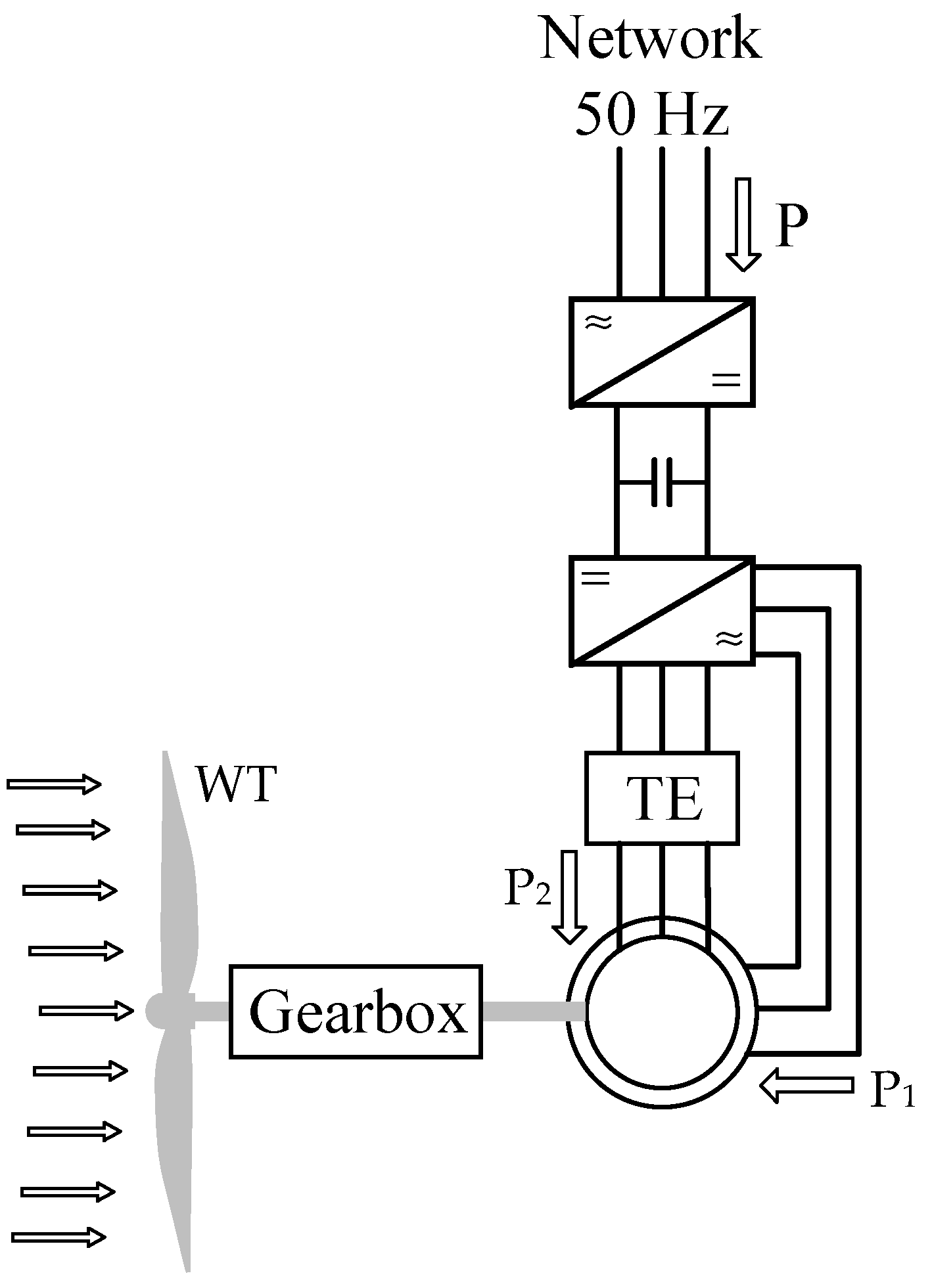
2. The Mathematical Model of the Double-Powered Induction Generator
- -
- Nominal power PN = PEG = 1.5 MW;
- -
- Nominal voltage, UN—690 V;
- -
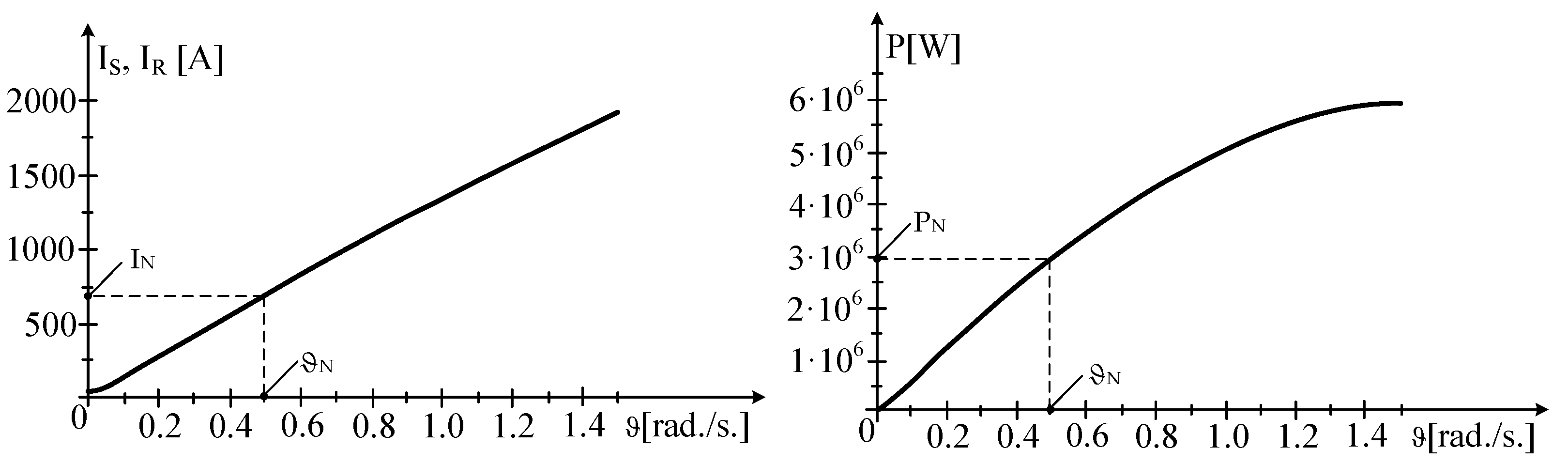
- Nominal current, IN = PEG/3UN = 1,500,000/3 · 690 = 724.64 A;
- -
- Nominal rotation, nN—1500 rpm.;
- -
- Maximum rotation, nmax—1800 rpm.;
- -
- Equivalent moment of inertia, J—136 [kgm2].
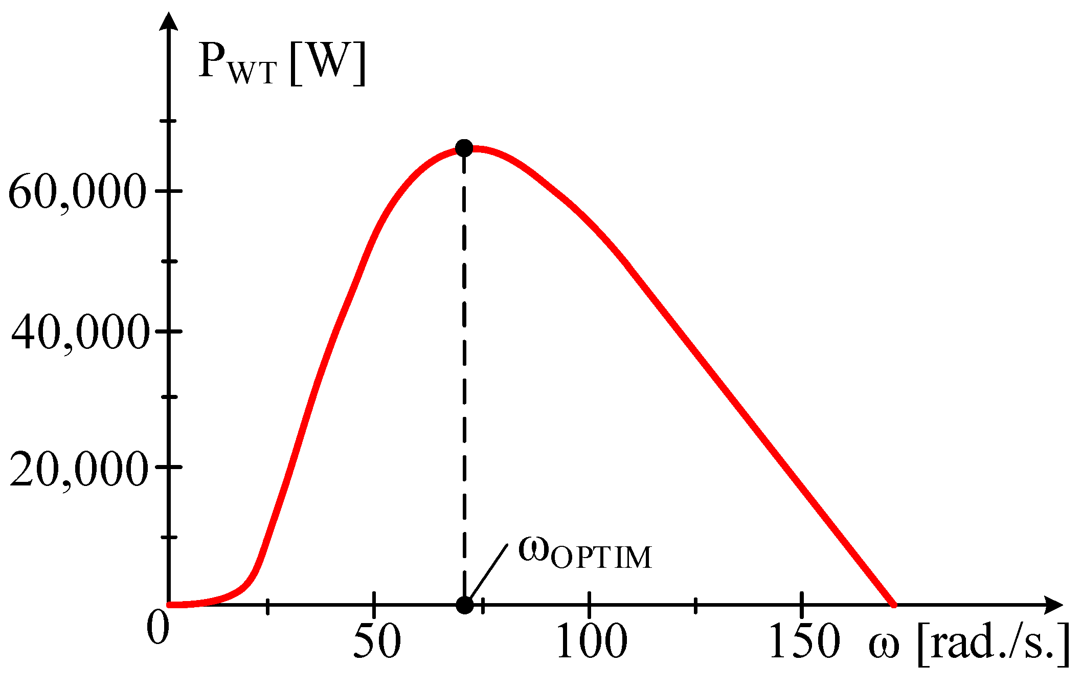
3. Mathematical Model of the Wind Turbine
4. Operating the Turbine by Switching the Generator to Engine Mode
- -
- disconnecting the EG from the grid (slower method);
- -
- switching the EG to engine mode (faster method).
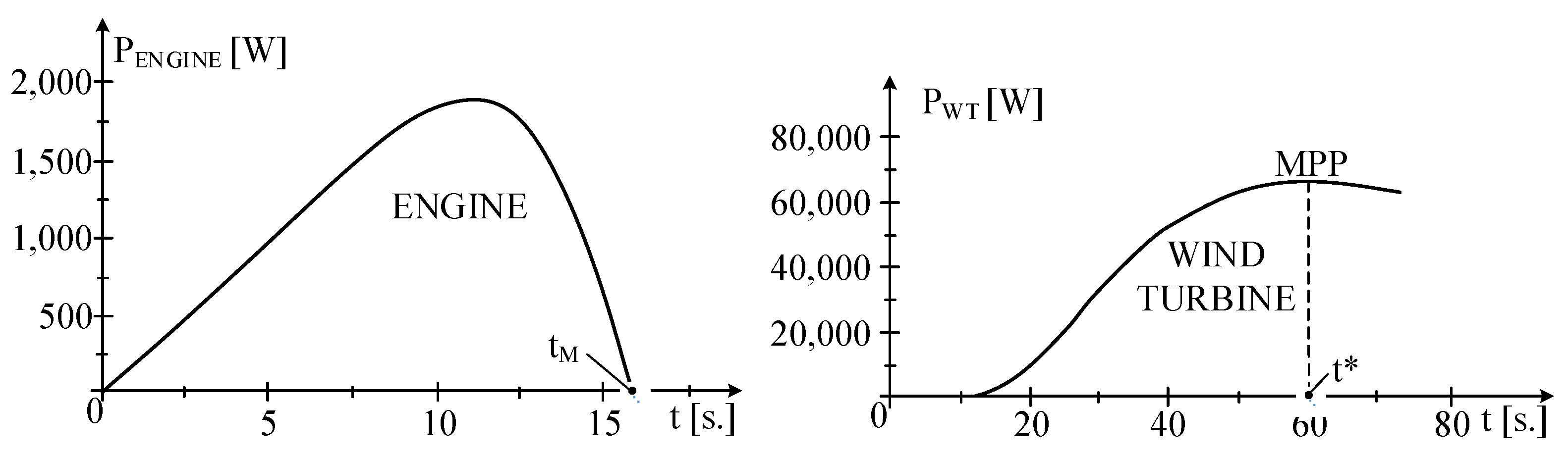
4.1. Case Study 1
- -
- only with the wind turbine and without power absorption from the network;
- -
- with wind turbine and motor, with power absorption from the grid.
4.1.1. Variant 1—Only with the Wind Turbine and Without Power Absorption from the Grid
4.1.2. Variant 2—With Wind Turbine and Motor with Power Absorption from the Network
4.2. Operation at Frequency Equality f1 = f2 = f
5. Mathematical Model of Dual Powered Asynchronous/Synchronous Motor
5.1. Stator Current Under Load and No-Load
5.2. Power to Synchronous Motor Shaft
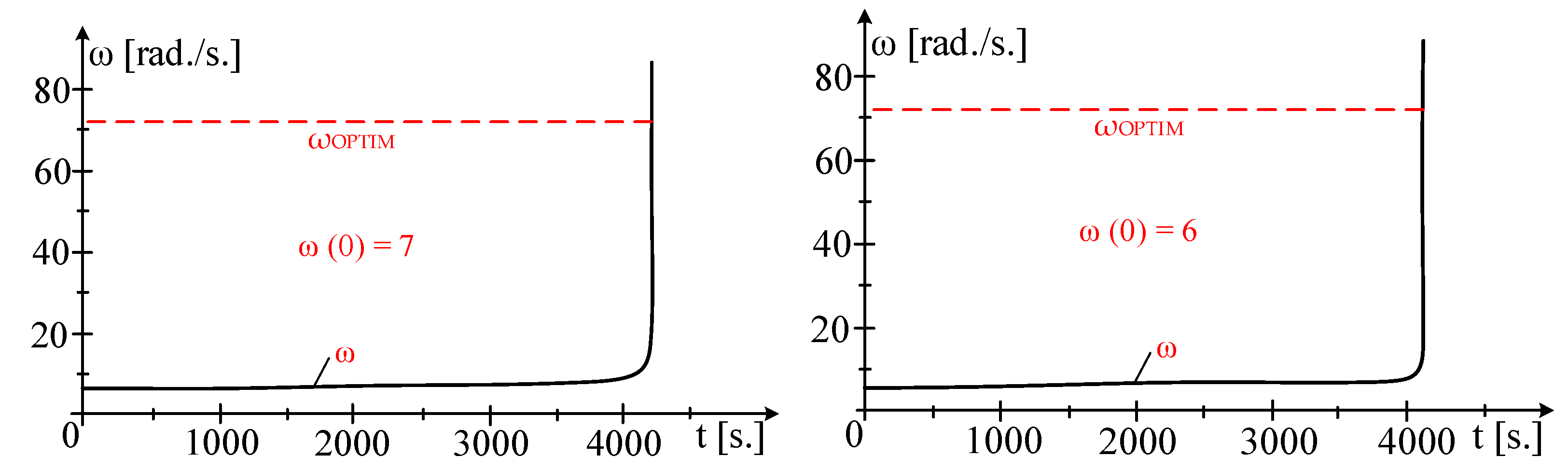
5.3. Visualization of the Process of Bringing It to the Optimal Rotational Speed
5.4. Achieving Optimal Speed and Switching to Generator Mode
5.5. Stationary Mode
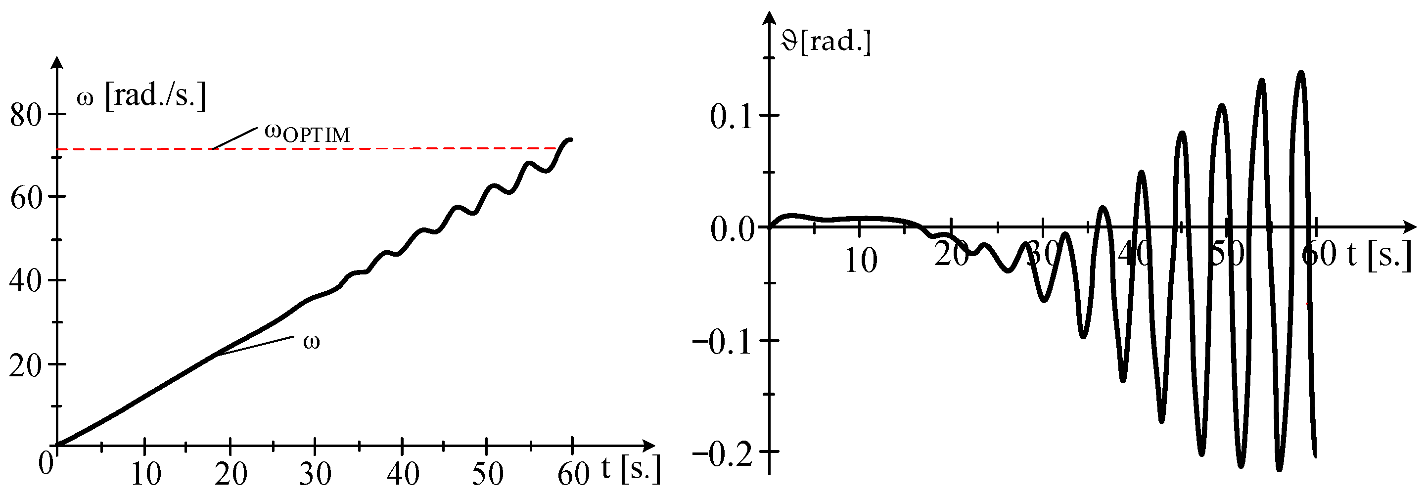
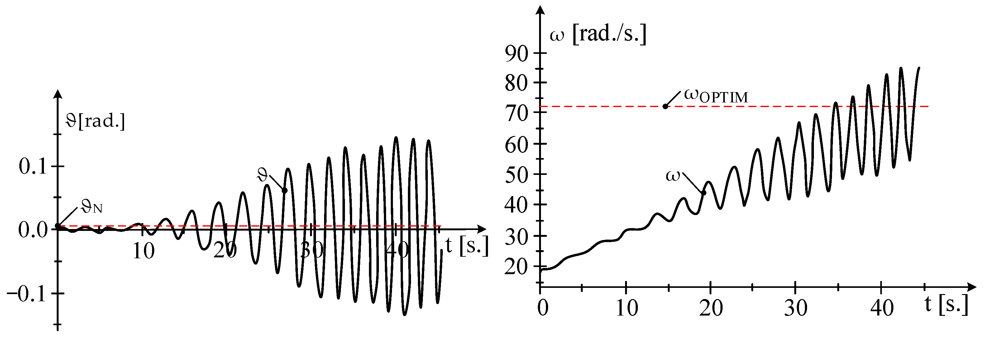
- At the beginning of the transient process, the mechanical angular speed, ω, and the charge angle, ϑ, vary linearly over time;
- At the end of the transient process, the mechanical angular speed, ω, and the charge angle, ϑ, vary oscillating over time;
- The oscillations of the load angle, ϑ, are more pronounced in cases where the motor is powered at variable voltage and frequency;
- The turbine enhances the fluctuations of the load angle, which are reflected in the variations in power output and current.
6. Discussion
- Develop a mathematical model for the wind turbine (WT) and the double-fed asynchronous/synchronous motor, derived from the induction generator with a wound rotor, utilizing experimental data as the foundation;
- Follow the transition of the asynchronous generator to a double-powered synchronous motor, with the stator and rotor connected to the same frequency network, so that the turbine operates at the point of maximum power in the shortest possible time interval;
- Visualize the process of bringing it to the optimal speed and interpreted the oscillations of the load angle and power at the double powered synchronous motor;
- Determine the oscillation of the load angle, the power when switching to generator mode as well as the operation at the maximum power point.
- When switching the asynchronous generator to the mode of a double-powered synchronous motor, at the same frequency, oscillations of the load angle and power occur;
- The most pronounced oscillations are in the stator and rotor power supply at variable frequency.
7. Conclusions
Author Contributions
Funding
Institutional Review Board Statement
Informed Consent Statement
Data Availability Statement
Conflicts of Interest
Abbreviations
| ω | mechanical angular speed |
| ωOPTIM | optimum angular speed |
| ωMAXIM | maximum angular speed |
| J | equivalent moment of inertia |
| PWT | power given by WT relative to the shaft of the electric motor/generator |
| PWT-MAX | maximum wind turbine power |
| PENGINE | electromagnetic power at the shaft of the induction motor |
| PN | nominal power |
| Psc | short-circuit power |
| PEG | power of the electric generator |
| P | mains power |
| P1 | power injected into the stator |
| P2 | power injected into the rotor |
| PS | active stator power |
| PR | active rotor power |
| UN | nominal voltage |
| US | stator voltage |
| UR | rotor voltage |
| IN | nominal current |
| Isc | short-circuit current |
| Ino-load | current from idle operation |
| IS | stator current |
| IR | rotor current |
| V | wind speed |
| nN | nominal rotation |
| nmax | maximum rotation |
| n1 | speed of the rotating field |
| n | rotational speed of the rotor |
| Zsc | short-circuit impedance |
| Rsc | short-circuit resistance |
| R1 | the resistance of the stator winding |
| R2 | the rotor winding resistance reduced to the stator |
| Xsc | short-circuit reactance |
| X1 | the reactance of the stator winding |
| X2 | the rotor winding reactance reduced to the stator |
| XM | magnetizing reactance |
| LM | magnetizing inductance |
| LS | stator inductance |
| LR | rotor inductance |
| s | slipping |
| N1 | number of turns per phase in the stator |
| N2 | number of turns per phase in the rotor |
| β | the angle of inclination of the blades |
| ρ | density of the air in the operating location |
| Rp | radius blades |
| Cp(λ) | power conversion coefficient |
| MM | mathematical model |
| kp | proportionality factor |
| f | frequency |
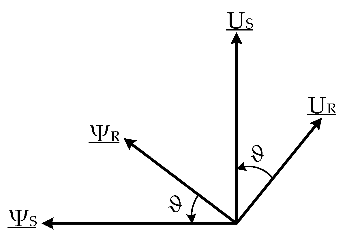
| ΨS | stator flux |
| ΨR | rotor flux |
| ϑ | load angle |
| σ | global dispersion factor |
| EG | electric generator |
| MWT | moment related to the shaft of the electric generator |
| MEG | electromagnetic torque at the electric generator |
| MPP | maximum power point |
| RES | renewable energy sources |
| POD | power oscillation damping |
| DFIG | double fed induction generator |
| WT | wind turbine |
| MAS | mechanical angular speed |
References
- Bishoge, O.K.; Zhang, L.L.; Mushi, W.G. The Potential Renewable Energy for Sustainable Development in Tanzania: A Review. Clean Technol. 2019, 1, 70–88. [Google Scholar] [CrossRef]
- Jamii, J.; Mimouni, F. Model of wind turbine-pumped storage hydro plant. In Proceedings of the 9th International Renewable Energy Congress (IREC), Hammamet, Tunisia, 20–22 March 2018. [Google Scholar]
- Khajah, A.M.H.A.; Philbin, S.P. Techno-Economic Analysis and Modelling of the Feasibility of Wind Energy in Kuwait. Clean Technol. 2022, 4, 14–34. [Google Scholar] [CrossRef]
- Sorandaru, C.; Muller, V.; Erdodi, M.G.; Edu, E.R.; Ancuti, M.C.; Musuroi, S.; Svoboda, M. Fundamental Issue for Wind Power Systems Operating at Variable Wind Speeds: The Dependence of the Optimal Angular Speed on the Wind Speed. In Proceedings of the International Conference and Exposition on Electrical And Power Engineering (EPE), Iasi, Romania, 20–22 October 2023. [Google Scholar]
- Pali, B.S.; Vadhera, S. An Innovative Continuous Power Generation System Comprising of Wind Energy Along with Pumped-Hydro Storage and Open Well. IEEE Trans. Sustain. Energy 2020, 11, 145–153. [Google Scholar] [CrossRef]
- Kambiz, T.; Milad, B.; Ali, M.-S.; Mo, J. A smart multiphysics approach for wind turbines design in industry 5.0. J. Ind. Inf. Integr. 2024, 42, 100704. [Google Scholar]
- Routray, A.; Hur, S.H. Power regulation of a wind farm through flexible operation of turbines using predictive control. Energy 2024, 313, 133917. [Google Scholar] [CrossRef]
- Deng, X.F.; Yang, J.; Sun, Y.; Song, D.R.; Yang, Y.G.; Joo, Y.H. An Effective Wind Speed Estimation Based Extended Optimal Torque Control for Maximum Wind Energy Capture. IEEE Access 2020, 8, 65959–65969. [Google Scholar] [CrossRef]
- Huynh, P.; Tungare, S.; Banerjee, A. Maximum Power Point Tracking for Wind Turbine Using Integrated Generator-Rectifier Systems. In Proceedings of the 11th Annual IEEE Energy Conversion Congress and Exposition (ECCE), Baltimore, MD, USA, 29 September–3 October 2019. [Google Scholar]
- Apostolos, G.P.; Apostolos, I.K.; Stavros, A.P. Solutions to Enhance Frequency Regulation in an Island System with Pumped-Hydro Storage Under 100% Renewable Energy Penetration. IEEE Access 2023, 11, 76675–76690. [Google Scholar]
- Apata, O.; Oyedokun, D.T.O. An overview of control techniques for wind turbine systems. Sci. Afr. 2020, 10, e00566. [Google Scholar] [CrossRef]
- An, Y.Y.; Li, Y.G.; Zhang, J.; Wang, T.; Liu, C.F. Enhanced Frequency Regulation Strategy for Wind Turbines Based on Over-speed De-loading Control. In Proceedings of the 5th Asia Conference on Power and Electrical Engineering (ACPEE), Chengdu, China, 4–7 June 2020. [Google Scholar]
- Rebello, E.; Watson, D.; Rodgers, M. Performance Analysis of a 10 MW Wind Farm in Providing Secondary Frequency Regulation: Experimental Aspects. IEEE Trans. Power Syst. 2019, 34, 3090–3097. [Google Scholar] [CrossRef]
- Edrah, M.; Zhao, X.W.; Hung, W.; Qi, P.Y.; Marshall, B.; Karcanias, A.; Baloch, S. Effects of POD Control on a DFIG Wind Turbine Structural System. IEEE Trans. Energy Convers. 2020, 35, 765–774. [Google Scholar] [CrossRef]
- Hua, Y.; Yujun, D.; Liye, X.; Qionglin, L.; Chen, Z.; Yi, W. Hydro-Tower Pumped Storage-based Wind Power Generator: Short-term Dynamics and Controls. In Proceedings of the 2nd Asian Conference on Frontiers of Power and Energy (ACFPE), Chengdu, China, 20–22 October 2023. [Google Scholar]
- Hussain, J.; Mishra, M.K. An Efficient Wind Speed Computation Method Using Sliding Mode Observers in Wind Energy Conversion System Control Applications. In Proceedings of the 8th IEEE International Conference on Power Electronics, Drives and Energy Systems (PEDES), Chennai, India, 18–21 December 2018. [Google Scholar]
- Youssef, B.; Seddik, B. DFIG-Based Wind Turbine Control Using High-Gain Observer. In Proceedings of the 1st International Conference on Innovative Research in Applied Science, Engineering and Technology (IRASET), Meknes, Morocco, 16–19 April 2020. [Google Scholar]
- Chioncel, C.P.; Chioncel, P.; Gillich, M.; Nierhoff, T. Overview of Classic and Modern Wind Measurement Techniques, Basis of Wind Project Development. Analele Univ. Eftimie Murgu Resita 2011, 3, 73–80. [Google Scholar]
- Sorandaru, C.; Musuroi, S.; Frigura-Iliasa, F.M.; Vatau, D.; Dordescu, M. Analysis of the Wind System Operation in the Optimal Energetic Area at Variable Wind Speed over Time. Sustainability 2019, 11, 1249. [Google Scholar] [CrossRef]
- Babescu, M. Sisteme automate de reglare. In Maşina sincronă: Modelare-Identificare-Simulare; Editura Politehnica Publisher: Timisoara, Romania, 2003; pp. 154–196. [Google Scholar]
- Yunus, Y.; Kambiz, T.; Mo, J. Wind Speed Forecasting using Machine Learning Approach based on Meteorological Data-A case study. Energy Environ. Res. 2022, 12, 11–25. [Google Scholar]
- Karthik, R.; Sri Hari, A.; Pavan Kumar, Y.V.; John Pradeep, D. Modelling and Control Design for Variable Speed Wind Turbine Energy System. In Proceedings of the 2020 International Conference on Artificial Intelligence and Signal Processing (AISP), Amaravati, India, 10–12 January 2020. [Google Scholar]
- Srinivasa Sudharsan, G.; Vishnupriyan, J.; Vijay Anand, K. Active flow control in Horizontal Axis Wind Turbine using PI-R controllers. In Proceedings of the 6th International Conference on Advanced Computing and Communication Systems (ICACCS), Coimbatore, India, 6–7 March 2020. [Google Scholar]
- Rezkallah, M.; Chandra, A.; Ibrahim, H. Wind-PV-Battery Hybrid Off-Grid System: Control Design and Real-Time Testing. Clean Technol. 2024, 6, 471–493. [Google Scholar] [CrossRef]
- Najih, Y.; Adar, M.; Aboulouard, A.; Khaouch, Z.; Bengourram, M.; Zekraoui, M. Mechatronic Control Model of a Novel Variable Speed Wind Turbine Concept with Power Splitting Drive Train: A Bond Graph Approach. In Proceedings of the 6th International Conference on Optimization and Applications (ICOA), Beni Mellal, Morocco, 20–21 April 2020. [Google Scholar]
- Fan, X.K.; Crisostomi, E.; Zhang, B.H.; Thomopulos, D. Rotor Speed Fluctuation Analysis for Rapid De-Loading of Variable Speed Wind Turbines. In Proceedings of the 20th IEEE Mediterranean Eletrotechnical Conference (IEEE MELECON), Electr Network, Palermo, Italy, 15–18 June 2020; pp. 482–487. [Google Scholar]
- Mohit, S.; Surya, S. Dynamic Models for Wind Turbines and Wind Power Plants; National Renewable Energy Laboratory: Golden, CO, USA, 2011. Available online: https://www.nrel.gov/docs/fy12osti/52780.pdf (accessed on 5 October 2024).
- Dobrin, E.; Ancuti, M.C.; Musuroi, S.; Sorandaru, C.; Ancuti, R.; Lazar, M.A. Dynamics of the Wind Power Plants at Small Wind Speeds. In Proceedings of the 14th International Symposium on Applied Computational Intelligence and Informatics (SACI), Timisoara, Romania, 21–23 May 2020. [Google Scholar]
- Chioncel, C.P.; Spunei, E.; Tirian, G.O. Visualizing the Maximum Energy Zone of Wind Turbines Operating at Time-Varying Wind Speeds. Sustainability 2024, 16, 2659. [Google Scholar] [CrossRef]
- Chioncel, C.P.; Spunei, E.; Tirian, G.O. The Problem of Power Variations in Wind Turbines Operating under Variable Wind Speeds over Time and the Need for Wind Energy Storage Systems. Energies 2024, 17, 5079. [Google Scholar] [CrossRef]
- Wind-Turbine-Models. Available online: https://en.wind-turbine-models.com/turbines/357-fuhrlaender-fl-md-77 (accessed on 6 November 2024).
- Song, Y.; Paek, I. Prediction and Validation of the Annual Energy Production of a Wind Turbine Using WindSim and a Dynamic Wind Turbine Model. Energies 2020, 13, 6604. [Google Scholar] [CrossRef]
- Boldea, I. Variable Speed Generators, 2nd ed.; Publisher Taylor & Francis Group: Abingdon, UK; CRC Press: Boca Raton, FL, USA, 2015; ISBN 978-1498723572. [Google Scholar]
- Yao, X.J.; Liu, Y.M.; Bao, J.Q.; Xing, Z.X. Research and Simulation of Direct Drive Wind Turbine VSCF Characteristic. In Proceedings of the IEEE International Conference on Automation and Logistics, Qingdao, China, 1–3 September 2008. [Google Scholar]
- Ragheb, M.; Ragheb, A.M. Wind Turbines Theory—The Betz Equation and Optimal Rotor Tip Speed Ratio. In Fundamental and Advanced Topics in Wind Power; Carriveau, R., Ed.; University of Windsor: Windsor, ON, Canada, 2011; pp. 19–38. [Google Scholar]
- Antar, E.; El Cheikh, A.; Elkhoury, M. A Dynamic Rotor Vertical-Axis Wind Turbine with a Blade Transitioning Capability. Energies 2019, 12, 1446. [Google Scholar] [CrossRef]
- Vadi, S.; Gürbüz, F.B.; Bayindir, R.; Hossain, E. Design and Simulation of a Grid Connected Wind Turbine with Permanent Magnet Synchronous Generator. In Proceedings of the 8th International Conference on Smart Grid (icSmartGrid), Paris, France, 17–19 June 2020. [Google Scholar]
- Carstea, C.; Butaru, F.; Ancuti, M.C.; Musuroi, S.; Deacu, A.; Babaita, M.; Stanciu, A.M. Wind Power Plants Operation at Variable Wind Speeds. In Proceedings of the 14th International Symposium on Applied Computational Intelligence and Informatics (SACI), Timisoara, Romania, 21–23 May 2020. [Google Scholar]
- Zhai, X.; Li, Z.; Li, Z.; Xue, Y.; Chang, X.; Su, J.; Jin, X.; Wang, P.; Sun, H. Risk-averse energy management for integrated electricity and heat systems considering building heating vertical imbalance: An asynchronous decentralized approach. Appl. Energy 2025, 353, 125271. [Google Scholar] [CrossRef]
- Zhang, H.; Li, Z.; Xue, Y.; Chang, X.; Su, J.; Wang, P.; Guo, Q.; Sun, H. A Stochastic Bi-Level Optimal Allocation Approach of Intelligent Buildings Considering Energy Storage Sharing Services. IEEE Trans. Consum. Electron. 2024, 70, 5142–5153. [Google Scholar] [CrossRef]


Disclaimer/Publisher’s Note: The statements, opinions and data contained in all publications are solely those of the individual author(s) and contributor(s) and not of MDPI and/or the editor(s). MDPI and/or the editor(s) disclaim responsibility for any injury to people or property resulting from any ideas, methods, instructions or products referred to in the content. |
© 2025 by the authors. Licensee MDPI, Basel, Switzerland. This article is an open access article distributed under the terms and conditions of the Creative Commons Attribution (CC BY) license (https://creativecommons.org/licenses/by/4.0/).
Share and Cite
Chioncel, C.P.; Spunei, E.; Tirian, G.-O. Wind Turbines Around Cut-In Speed: Startup Optimization and Behavior Analysis Reported to MPP. Appl. Sci. 2025, 15, 3026. https://doi.org/10.3390/app15063026
Chioncel CP, Spunei E, Tirian G-O. Wind Turbines Around Cut-In Speed: Startup Optimization and Behavior Analysis Reported to MPP. Applied Sciences. 2025; 15(6):3026. https://doi.org/10.3390/app15063026
Chicago/Turabian StyleChioncel, Cristian Paul, Elisabeta Spunei, and Gelu-Ovidiu Tirian. 2025. "Wind Turbines Around Cut-In Speed: Startup Optimization and Behavior Analysis Reported to MPP" Applied Sciences 15, no. 6: 3026. https://doi.org/10.3390/app15063026
APA StyleChioncel, C. P., Spunei, E., & Tirian, G.-O. (2025). Wind Turbines Around Cut-In Speed: Startup Optimization and Behavior Analysis Reported to MPP. Applied Sciences, 15(6), 3026. https://doi.org/10.3390/app15063026