Abstract
In this paper, we present a method for obtaining a manifold color correction transform for multiview images. The method can be applied in various scenarios, for correcting the colors of stitched images, adjusting the colors of images obtained in different lighting conditions, and performing virtual view synthesis based on images taken by different cameras or in different conditions. The provided derivation allows us to use the method to correct regular RGB images. The provided solution is specified as a transform matrix that provides the pixel-specific color transformation for each pixel and therefore is more general than the methods described in the literature, which only provide the transformed images without explicitly providing the transform. By providing the transform for each pixel separately, we can introduce a smoothness constraint based on the transformation similarity for neighboring pixels, a feature that is not present in the available literature.
1. Introduction
In many applications, we use multiple acquisition devices to record images of the same object. This results in multiple images of the same object with different gamut/color characteristics. Even a single camera can capture images with different colorings due to changing weather conditions. This variation affects image or object recognition algorithms, panorama creation, image stitching, virtual view creation, or Neural Radiance Field (NeRF) [1,2] estimation. To address these differences, color calibration is necessary. It allows us to find a mapping of colors from one image to another. Various methods exist to achieve this mapping or transformation. Nearly all of them assume constant color transformation across the whole image. In this paper, we are presenting a novel manifold color calibration method that allows per-pixel color transformation estimation between pairs of images, even when in partially occluded image pairs.
For example, in low-light conditions, we can take a dark color image and a near-infrared image of the same object [3], or take a shot with and without a flash [4] and then try to combine both of the images together.
Another example would be applications in view synthesis [5,6], where we can create a non-existing view of the scene from the viewpoint of so-called virtual cameras based on two (or more) images captured by real cameras recording the given scene. Even if both cameras are identical (which is not always possible), they can produce images with different color characteristics. This could happen even due to the different viewpoints from which the images were taken.
Although the problem is the most obvious for multi-camera scenarios, using a single camera can also lead to the different colorings of the captured images, for example, due to the changing weather conditions. In applications such as image/object recognition, this could significantly influence the performance of the algorithms used.
Yet another example is panorama creation or/and image stitching [7]. Where we can stitch or combine multiple images captured either by the same image sensor or by multiple sensors into one big continuous image.
In all the abovementioned situations, we can color calibrate the images in order to minimize the artifacts occurring due to the color mismatch. This can be performed by finding the mapping of colors from one image to the other.
There already exist many methods of finding such mappings or transformations, which map the color of all pixels from one image to the other.
The significance of color correction manifests itself in many applications, where different methods were demonstrated to effectively improve the performance of the whole system. One such example is multiview video compression, as evidenced in [8,9,10,11]. In those papers, the authors demonstrate an improvement in the coding of the multiview video after applying a preprocessing step of color matching of the sequences due to the improved accuracy of motion compensation and inter-view prediction.
The methods used to perform the color correction that is described in the literature can be based on histogram equalization [11,12,13]. A popular method is also using a single scaling factor, correction coefficient, or a polynomial to correct for the color differences [14,15,16,17]. A low-dimensional matrix correction can also be used [18]. Another way to color correct the images is to use the color transfer technique [19]. In recent years, neural networks have been used to perform similar tasks and can be used to perform color transfer as well; an example of this color transfer method can be found in [20].
In practice, it is important to not only correct the colors of the images but also maintain sufficient quality of the corrected images without degrading the contrast of the processed images [21]. Thus, the correction algorithm should also consider the texture/contrast information in the processed images.
Another way of performing the color correction is to solve a manifold optimization problem defined globally for the entire image. Such an approach can be found in [8,22,23]. The authors of [8,23] define color correction as an optimization problem with priors both from the source image and from the target image. From the source image, the priors are color characteristics and color distribution, while from the target image, the priors tend to preserve the spatial and temporal structure of the image, after color correction. Similarly, the paper [22] introduces a method for global optimization of pixel values for large baseline multiview sequences, preserving the structure and spatio-temporal consistency.
The paper [24] introduces a parametric linear method and a nonparametric nonlinear method to deal with different color changes between pairs of images. The method proposed is a modified Laplacian Eigenmaps, which is a nonlinear manifold learning approach. The used goal function for color transfer is a quadratic cost function with a quadratic regularizer. The described method only searches for image sample values of a target image, matching the color characteristics of a source image.
In many applications, only a fraction of the pixels from one image directly correspond to any other image. For example, in image stitching, images only partially overlap. Similarly, in view synthesis, synthesized images from a virtual camera contain holes caused by disocclusions, where some parts of the scene are not visible due to perspective changes between the source view and the virtual view created with the source view data. Thus, only part of the real image has corresponding pixels in the virtual image. Yet we can obtain color transformation for all of the pixels in the images in order to seamlessly combine them together.
Color characteristics can vary across images due to effects like ambient occlusion, nonuniform lighting, shadows, and non-Lambertian reflections. Most color calibration techniques do not work reliably for these cases, only averaging color distribution and color characteristics across entire images. But in many applications, we can retain that non-uniformity during the color transformation from one image to the other, since they are inherent for some objects and materials. We can preserve these features for a color-corrected view.
To obtain a proper transformation that preserves the aforementioned effects, one needs to estimate per-pixel color transformation from one image to the other. An important factor of novelty of the work presented in this paper is the fact that the optimization algorithm does not work on the pixel values themselves, but rather on the transformations applied to those pixels. In this way, our method can use optimization constraints that do not refer to pixel values, but rather to the transformations that are applied to the pixel values. In this way, it is possible to obtain a smooth transformation field that can better capture the specific properties of a given scene. Additionally, the presented method includes parameters that can be used to adjust the smoothness of the transformation manifold. We also provide values of the parameters that were found to provide good results for all the tested sequences.
In this paper, we describe such a method and provide experimental results obtained with the use of the method.
In this paper, we first present the formal description of the optimization problem in a simple abstract space and then provide an analytical solution for this space.
From there, we move on to a more complex case, where the problem is defined in a 2D grid, normally used in image and video processing. We present the problem formulation in this 2D grid space and provide a solution for such a space.
The final part of derivation considers the occlusions and non-overlapping parts of the scene, the phenomena usually encountered in practical applications. The solution provided for the 2D grid is therefore modified to deal with occlusions and provide accurate transformation for those parts of the image, even in case of the absence of correspondence data.
The rest of the paper is organized as follows: Section 2 defines formally the actual problem, Section 3 provides an analytical solution, Section 4 describes the same problem in a 2D grid that is commonly used in digital images, Section 5 provides the solution for a 2D grid, Section 6 provides information about the application for occluded parts of the virtual image, Section 7 provides experimental results performed with the use of the described method, and Section 8 summarizes the entire paper with conclusions.
2. Problem Definition
Let us assume we have two images, left and right, that represent the same viewpoint of a scene. Let us assume that and are n-component vectors of colors of pixel p in the left and right images. The n denotes the number of components in an image increased by 1 since the operations are performed in homogenous coordinates, which offer more flexibility over regular cartesian coordinates. Therefore, commonly n will be 4 for homogenous coordinates of RGB color space.
We would like to estimate a manifold of per-pixel transformation such that for all pixels p
where
For an RGB image, the matrix will be a 4 × 4 (since we are operating in homogenous coordinates, as explained before), and there is a p such matrix, one for every pixel in the image (p is the number of pixels in the image). Please note that at this stage, the matrix is agnostic to the way the pixels are organized in the image since p is merely an index.
In the further part of the derivation, we will continue to use n as the size of the matrix Ap since the method can be applied not only to RGB images but potentially also to multispectral and hyperspectral images.
The problem considered in this paper is to find the transformation for a given pair of images, e.g., coming from a pair of cameras in stereoscopic applications.
3. Derivation of the Solution
Because the system of Equation (1) for every pixel is under-determined, we can define the minimization problem with a goal function . We can transform color of left image pixel through as close as possible to the color of the right image pixel with the same pixel index
where is the Euclidean norm.
Moreover, we can have a smooth manifold , which means that the two transformations and for two neighboring pixels or should be similar. It means that both transformations applied to one (any) of those pixels should give the same result (or at least as close as possible). We denote as any of the two pixels or
So, finally, we can minimize the difference (3). We compute the derivative of (3) with respect to every element of manifold
All derivatives with respect to from the sum in (5) except are equal to from which follows that
Lemma 1.
Assume some vector then the square of Euclidean norm is:
So, any derivative of a square of Euclidean norm of this vector can be expressed as:
Using Lemma 1 in (6), we have
Lemma 2.
Let us define a vector in which all components are 0 except for -th, which is 1. Now, we can calculate the derivative of matrix with respect to its element
Because all matrix components are independent of except element, so
So, using Lemma 2 in (9), we have
Lemma 3.
Let us define a vector in which all components are 0 except for -th, which is 1. Now, we can define the selection of -th component as:
where L is an component vector.
where is by matrix and mean -th row of a matrix .
Using Lemma 3 on (11), we have
Similarly, we would like to minimize (4). So, we compute the derivative of (4) with respect to every element of manifold
All derivatives with respect to from the sum in (15) except for the pair and are equal to , so
Using Lemma 1 in (16), we have
Using Lemma 2 in (17), we have
Using Lemma 3 on (18), we have
Similarly, we compute the derivative of (4) with respect to every element of manifold
All derivatives with respect to from the sum in (20) except for the pair and are equal to so
Using Lemma 1 in (21), we have
Using Lemma 2 in (22), we have
Using Lemma 3 on (23), we have
In order to estimate manifold , we create a system of equations for pixel
We can express (25) as
where is a vector composed of all coefficients of the matrix , and vector is defined as follows
And the matrix is a block-based matrix composed of defined as follows
For a manifold composed of pixels, we can define the system of Equation (25) using the Formula (26) as
where and are a concatenation of and for all pixels in the image
And can be defined as a block matrix composed of
Similarly, in order to estimate manifold based on , we create a system of Equations (19) and (24) for pixel and q
Using a definition of given in (29), we can rewrite Equation (33) as
The exact formulation of matrix for all of the pixels depends strongly on the relationship between the position of pixels and .
4. Formulation in 2D Pixel Grid
Suppose we have an image of size by and we can indicate the pixel position by its coordinates in the image. Moreover, suppose that we introduce 2 smoothness constraints: one vertical and one horizontal. It means that pixel and have two neighboring pixels in which the coordinate differs only by 1.
Similarly, pixel and have two neighboring pixels whose u coordinate differs only by 1.
Moreover, we will assume that condition (34) is reflective and must hold for both pixels and , so:
will lead to
Combining both (38) and (39) together results in
After making such assumptions, we can provide an explicit form of , vectors, and matrix for any given pixel based on (31), (32), and (40). As the conditions and need to be satisfied simultaneously, we introduce two coefficients and to control the strength of the smoothness prior to in both directions on the 2D grid. The values of coefficients and were experimentally adjusted for universally good results among the tested sequences. The value of 0.1 was found to work well in our experiments, independent of the sequence contents and scene complexity. It needs to be stressed, however, that different resolutions of the sequences may require a slight modification of the values, but we found during the experiments that the method is not sensitive to the actual value of the coefficients and .
The final form of Equation (43) for all of the pixels is just a sum of (41) and (42)
5. Solution on a 2D Grid
The solution of obtained Equation (43) is simply given by
However, solving for on an average image is not an easy task. For a typical RGB image of resolution 1920 × 1080 vectors have the size of and the square matrix is of that same size. The main problem is to inverse the matrix, mainly because it is so enormous.
Fortunately, matrix is also vastly sparse with most of its coefficients located along the first, second, and W-diagonal (where W stands for the width of the image under consideration). There are many algorithms for efficient inversing (or pseudo-inversing) such huge sparse matrices.
In the experiments further on we have used Transpose-Free Quasi-Minimal Residual Algorithm [25,26,27].
After solving Equation (43) for we obtained an estimation of the manifold of per-pixel transformation allowing per-pixel color transformation between both of the images.
This allows the transformation of one image into a color space of the other, retaining its local color characteristics. After transformation, depending on the use case, one can directly output the transformed image as the final result, as can be performed in the “flash–no flash” application, merge them via some kind of blending or averaging, or inpaint one of the images by the content of the other or stitch them together to create a larger panorama.
6. Notes on Partially Overlapping Images
In the case of partially overlapping images like in the case of image stitching or view synthesis, a form of the matrix and the vector needs to be adjusted. Without loss of generality, let us assume that the left image is more complete, i.e., it has pixels in places where the right image does not. So, there are two possibilities: either left and right images do not have a given pixel or just the right pixel is not available. In both cases, for these pixels’ positions, condition cannot be used due to a lack of explicit pixel correspondence. In the second case, depending on the surroundings, we have pixel color values in the left image that can be used in condition for smooth manifold estimation.
For the first case, is as shown in (46)
In the second case, the is given as (47)
7. Experiments
The foundation of our experiments was the reference virtual view synthesis software VSRS [28]. It should be noted that VSRS does not include any color correction algorithm. Our algorithm was implemented within this software package.
We modified the post-processing only after the forward depth map projection step and the backward texture warping step had been carried out, and before the inpainting step.
For our testing, we employed several well-known and recognizable multiview test sequences equipped with high-quality depth maps. This set includes linear and arc multiview content. Used multiview test sequences exhibit a whole range of effects like ambient occlusions, nonuniform lighting, shadows, and non-Lambertian reflections. Table 1 lists the sequences used in the experiment.

Table 1.
Test sequences used in the experiment.
We rendered virtual views using the original VSRS and VSRS implementing our method. The virtual views were generated from data from the two views specified as the right and left views in Table 1. The set of data consists of the images, depth maps, and camera parameters. The virtual view matched the position of the third camera used during sequence acquisition.
The quality of the resulting virtual view has been measured as a luminance PSNR value of the virtual view generated with respect to the view recorded by the real camera at the same spatial position. The numerical results are presented in Table 2. A demonstration of the improvement provided by our method over the original method is shown in Figure 1, where details of the virtual views are compared.
Table 2.
Quality (PSNR) of the virtual views.
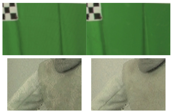
Figure 1.
Details of the virtual views: Top row: Poznan Blocks, Bottom row: Poznan Fencing 2. Original VSRS on the left, modified VSRS with proposed color correction on the right. As can be seen on the right-hand side images, most of the artifacts due to color mismatch are eliminated.
It can clearly be seen that the presented method significantly improves the quality of a virtual view by providing consistent colors of the pixels from different views. The artifacts stemming from slight differences between the color characteristics of the cameras and/or lighting conditions are reduced significantly.
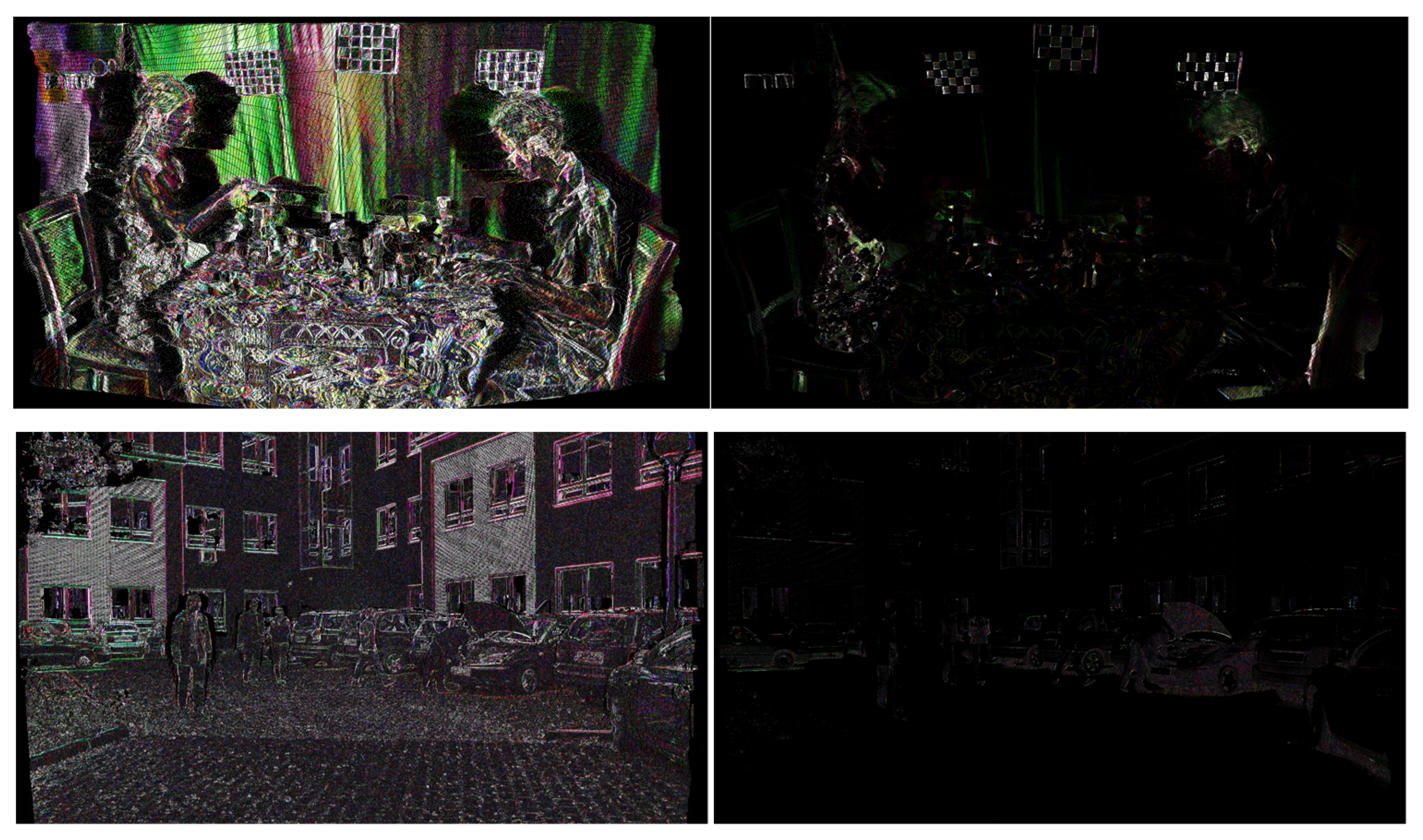
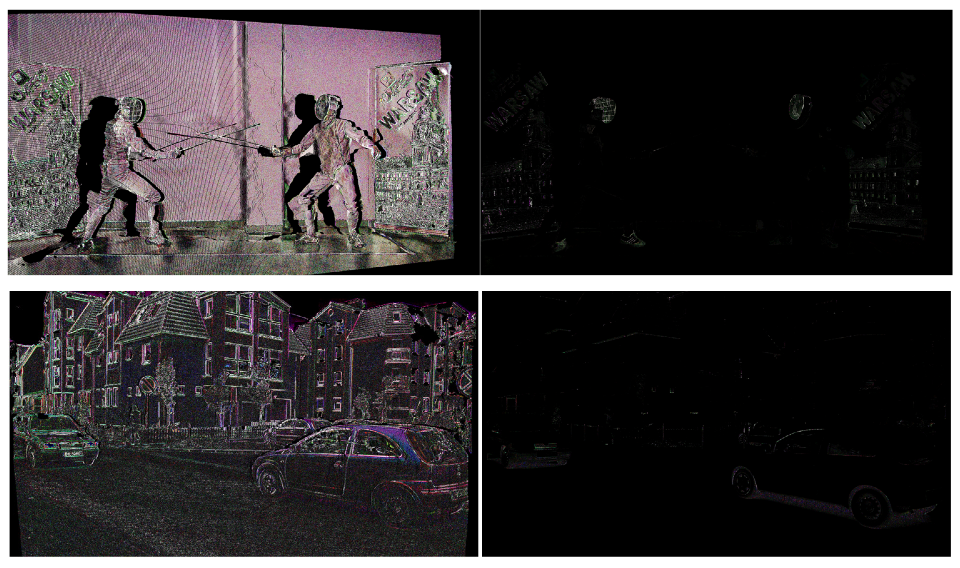
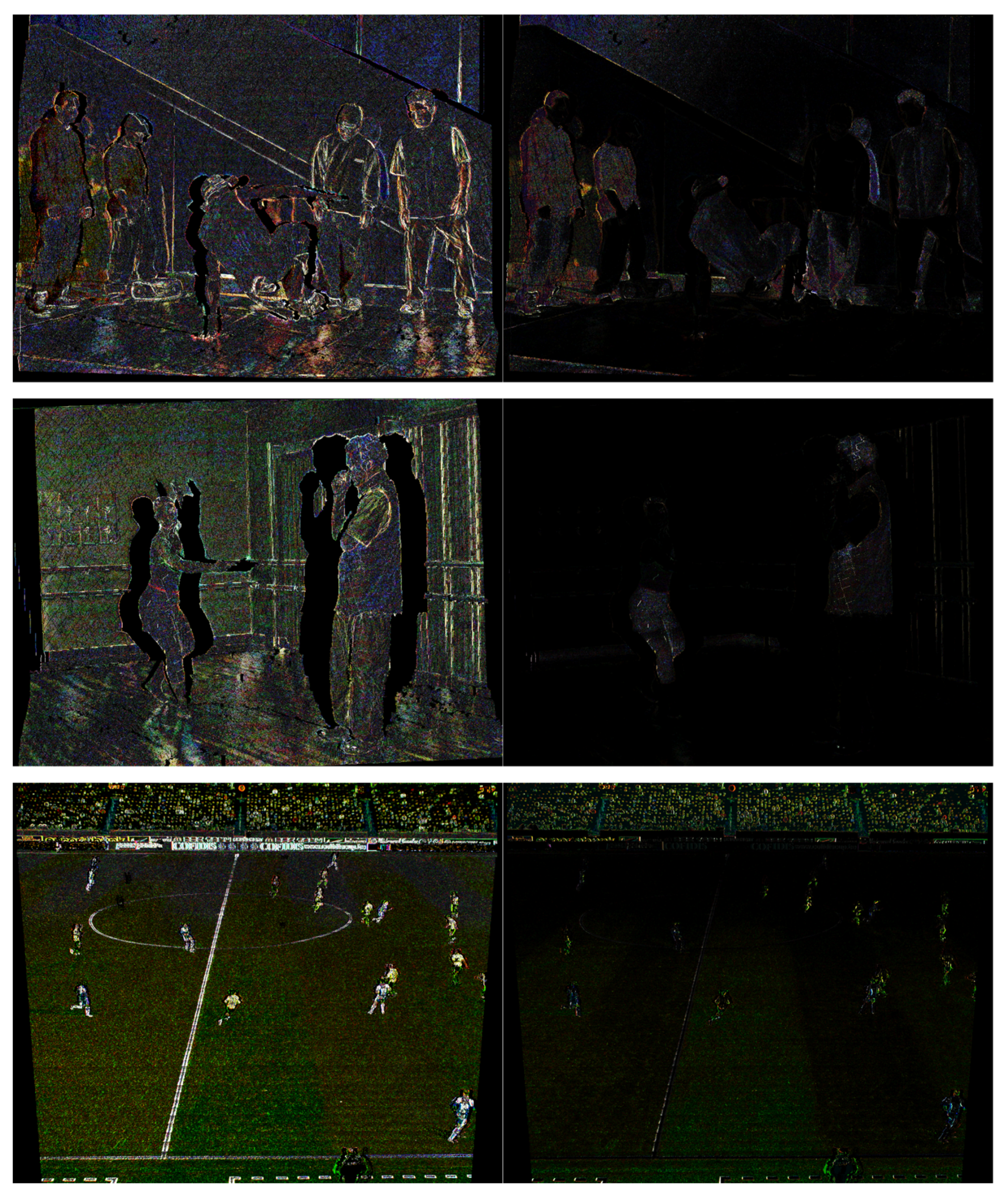
The PSNR value measured against a real view is a commonly used measure of quality for virtual view synthesis research. For color correction algorithms, however, a more significant figure of merit would be the comparison between the virtual view synthesized only from the left and only from the right view. Table 3 shows the values of the error (measured as a mean value of SSD for pixel values) for the virtual view generated from the left view calculated against the virtual view generated from the right view for three cases: no color correction applied, the global color correction applied according to the method described in [33], and the proposed method. A visual comparison of the differences between the virtual view generated from the left view and the virtual view generated from the right view is presented in Figure 2 and Figure 3. The proposed method outperforms significantly the global color correction method.
Table 3.
Mean values of SSD for the virtual view generated from the left view compared to the virtual view generated from the right view.
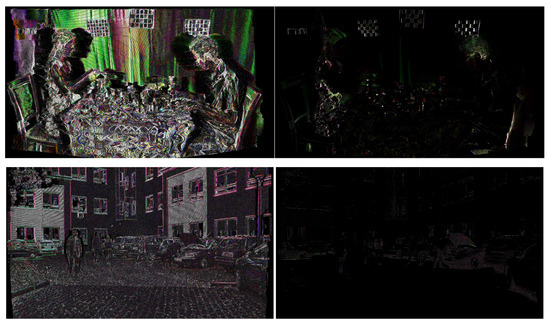
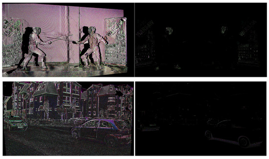
Figure 2.
Comparison of the differences between the virtual view generated from the left view and the virtual view generated from the right view: Left column—original VSRS, right column—modified VSRS. From the top: Poznan Blocks, Poznan Street, Poznan Fencing 2, Poznan Carpark.
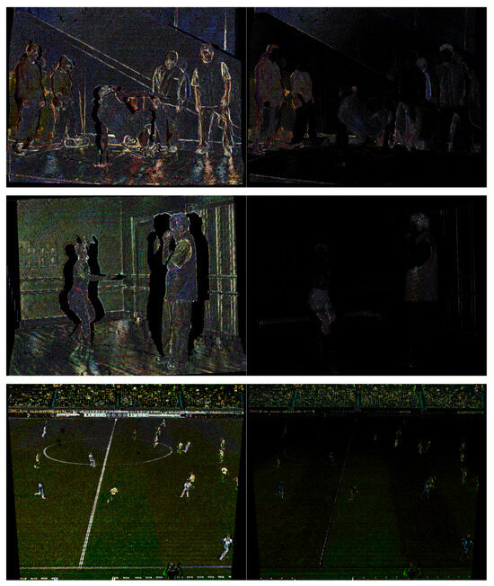
Figure 3.
Comparison of the differences between the virtual view generated from the left view and the virtual view generated from the right view: Left column—original VSRS, right column—modified VSRS. From the top: Breakdancer, Ballet, Soccer.
In order to test our method in a flash/no-flash scenario, we use the images from [4], as supplied in [34]. The proposed method of estimating per-pixel color transfer manifold can be used to correct images captured with flash to its low-light ambient counterpart, to match the no-flash colors (Figure 4).
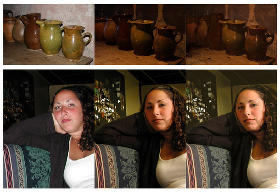
Figure 4.
Results of the proposed method for images with different lighting conditions. From the left: image with flash, no-flash image, result of our color-correction of the image with flash.
As can be seen, the proposed method is able to perform the color correction of the flash image so that it matches the colors of the image taken without flash. It can be seen that the artifacts common to images taken with flash, as non-Lambertian reflections are correctly processed.
8. Summary
In the paper, we have presented a new formulation of the per-pixel color calibration between images. The presented method can be applied to images with an arbitrary number of channels due to the flexibility and generalization provided by our derivation. The proposed algorithm is based on per-pixel manifold color transformation estimation. The proposed algorithm estimated a smooth manifold of color transformations across the whole image, even in the case when not all pixels have correspondence. The method allows for color profile mapping in difficult areas, like occluded regions of images, in shadows, and in the presence of reflections and a non-uniform lighting. The proposed method provides a gain in objective quality measure PSNR of 1.10 dB on average over seven different test sequences. The proposed method provided improvement for all tested sequences; the quality increase was in the range from 2.83 dB to 0.15 dB. The explanation of the differences may be attributed qualitatively to the different lighting conditions. Smaller improvements were observed for outdoor sequences recorded during a cloudy day, with no bright sun, and for sequences with uniform ambient lighting. For sequences with artificial light, the improvement was significantly larger. The subjective quality increase is also significant, as presented by the images in Figure 1 and Figure 4.
Much more improvement due to the use of the proposed method is observed when SSD between the virtual view synthesized from the left view is compared to the view synthesized from the right view. Here, when compared to the no color correction scenario, the reduction was more than 20-fold, with a maximum of 87-fold SSD reduction. When compared to a scenario where a competing method [33] is used, the SSD reduction is from 19.8-fold to 79.9-fold.
The presented method is envisaged to be applied as a preprocessing step in a post-production phase, since the computational complexity is significant, the most time-consuming part being the large sparse matrix inversion. While real-time image processing was beyond the scope of this work, it is worth noting that faster matrix inversion methods exist, which would reduce the computational complexity of our method.
The method significantly improves the quality of the virtual view synthesized from the multi-camera setups by applying color correction to all original views. It can be used in immersive video applications, where it can greatly reduce the color mismatch between camera views. It is also useful for single images in the scenario, flash–no flash images, as evidenced in the experiments.
Author Contributions
Conceptualization, K.W. and T.G.; methodology, S.G.; software, K.W.; validation, S.G., T.G. and K.K.; formal analysis, S.G.; investigation, T.G. and K.K.; writing—original draft preparation, K.W.; writing—review and editing, T.G. and K.K. All authors have read and agreed to the published version of the manuscript.
Funding
Project funded by The National Centre for Research and Development in the LIDER Programme (LIDER/34/0177/L-8/16/NCBR/2017). The work was supported by the Ministry of Science and Higher Education, Poland.
Institutional Review Board Statement
Not applicable.
Informed Consent Statement
Not applicable.
Data Availability Statement
The original contributions presented in the study are included in the article, further inquiries can be directed to the corresponding author.
Conflicts of Interest
Author Krzysztof Wegner was employed by the company Mucha sp. z o.o. The remaining authors declare that the research was conducted in the absence of any commercial or financial relationships that could be construed as a potential conflict of interest.
References
- Mildenhall, B.; Srinivasan, P.P.; Tancik, M.; Barron, J.T.; Ramamoorthi, R.; Ng, R. NeRF: Representing scenes as neural radiance fields for view synthesis. Commun. ACM 2021, 65, 99–106. [Google Scholar] [CrossRef]
- Wang, P.; Liu, Y.; Chen, Z.; Liu, L.; Liu, Z.; Komura, T.; Theobalt, C.; Wang, W. F2-nerf: Fast neural radiance field training with free camera trajectories. In Proceedings of the IEEE/CVF Conference on Computer Vision and Pattern Recognition, Vancouver, BC, Canada, 17–24 June 2023; pp. 4150–4159. [Google Scholar]
- Nawaz, A.; Kanwal, I.; Idrees, S.; Imtiaz, R.; Jalil, A.; Ali, A.; Ahmed, J. Fusion of color and infrared images using gradient transfer and total variation minimization. In Proceedings of the 2nd International Conference on Computer and Communication Systems (ICCCS), Krakow, Poland, 11–14 July 2017; pp. 82–85. [Google Scholar] [CrossRef]
- Petschnigg, G.; Szeliski, R.; Agrawala, M.; Cohen, M.; Hoppe, H.; Toyama, K. Digital photography with flash and no-flash image pairs. ACM Trans. Graph. 2004, 23, 664–672. [Google Scholar] [CrossRef]
- Furukawa, Y.; Hernández, C. Multi-View Stereo: A Tutorial. Found. Trends® Comput. Graph. Vis. 2015, 9, 1–148. [Google Scholar] [CrossRef]
- Li, Y.; Li, Y.; Yao, J.; Gong, Y.; Li, L. Global Color Consistency Correction for Large-Scale Images in 3-D Reconstruction. IEEE J. Sel. Top. Appl. Earth Obs. Remote Sens. 2022, 15, 3074–3308. [Google Scholar] [CrossRef]
- Chung, K.-L.; Lee, C.-Y. Fusion-Based Multiview Color Correction via Minimum Weight-First-Then-Larger Outdegree Target Image Selection. IEEE Trans. Geosci. Remote Sens. 2024, 62, 4707716. [Google Scholar] [CrossRef]
- Lu, S.-P.; Ceulemans, B.; Munteanu, A.; Schelkens, P. Spatio-Temporally Consistent Color and Structure Optimization for Multiview Video Color Correction. IEEE Trans. Multimed. 2015, 17, 577–590. [Google Scholar] [CrossRef]
- Chen, Y.; Cai, C.; Liu, J. YUV Correction for Multi-View Video Compression. In Proceedings of the 18th International Conference on Pattern Recognition (ICPR’06), Hong Kong, China, 20–24 August 2006; pp. 734–737. [Google Scholar] [CrossRef]
- Fezza, S.A.; Larabi, M.-C.; Faraoun, K.M. Coding and rendering enhancement of multi-view video by color correction. In Proceedings of the European Workshop on Visual Information Processing (EUVIP), Paris, France, 10–12 June 2013; pp. 166–171. [Google Scholar]
- Fezza, S.A.; Larabi, M.-C. Color calibration of multi-view video plus depth for advanced 3D video. Signal Image Video Process. 2015, 9, 177–191. [Google Scholar] [CrossRef]
- Ganelin, I.; Nasiopoulos, P. Virtual View Color Estimation for Free Viewpoint TV Applications Using Gaussian Mixture Model. In Proceedings of the 25th IEEE International Conference on Image Processing (ICIP), Athens, Greece, 7–10 October 2018; pp. 3898–3902. [Google Scholar] [CrossRef]
- Ding, C.; Ma, Z. Multi-Camera Color Correction via Hybrid Histogram Matching. IEEE Trans. Circuits Syst. Video Technol. 2021, 31, 3327–3337. [Google Scholar] [CrossRef]
- Joshi, N. Color Calibration for Arrays of Inexpensive Image Sensors, Technoly Report; CSTR 2004-02 3/31/04 4/4/04; Stanford University: Stanford, CA, USA, 2004. [Google Scholar]
- Suominen, J.; Egiazarian, K. Camera Color Correction Using Splines. Electron. Imaging 2024, 36, 165-1–165-6. [Google Scholar] [CrossRef]
- Qiao, Y.; Jiao, L.; Yang, S.; Hou, B.; Feng, J. Color Correction and Depth-Based Hierarchical Hole Filling in Free Viewpoint Generation. IEEE Trans. Broadcast. 2019, 65, 294–307. [Google Scholar] [CrossRef]
- Dziembowski, A.; Mieloch, D.; Różek, S.; Domański, M. Color Correction for Immersive Video Applications. IEEE Access 2021, 9, 75626–75640. [Google Scholar] [CrossRef]
- Ilie, A.; Welch, G. Ensuring color consistency across multiple cameras. In Proceedings of the Tenth IEEE International Conference on Computer Vision (ICCV’05) Volume 1, Beijing, China, 17–21 October 2005; Volume 2, pp. 1268–1275. [Google Scholar] [CrossRef]
- Reinhard, E.; Adhikhmin, M.; Gooch, B.; Shirley, P. Color transfer between images. IEEE Comput. Graph. Appl. 2001, 21, 34–41. [Google Scholar] [CrossRef]
- Flynn, J.; Neulander, I.; Philbin, J.; Snavely, N. DeepStereo: Learning to Predict New Views From the World’s Imagery. arXiv 2016, arXiv:1506.06825. [Google Scholar] [CrossRef]
- Li, Y.; Li, L.; Yao, J.; Xia, M.; Wang, H. Contrast-Aware Color Consistency Correction for Multiple Images. IEEE J. Sel. Top. Appl. Earth Obs. Remote Sens. 2022, 15, 4941–4955. [Google Scholar] [CrossRef]
- Ye, S.; Lu, S.-P.; Munteanu, A. Color correction for large-baseline multiview video. Signal Process. Image Commun. 2017, 53, 40–50. [Google Scholar] [CrossRef]
- Ceulemans, B.; Lu, S.-P.; Schelkens, P.; Munteanu, A. Globally optimized multiview video color correction using dense spatio-temporal matching. In Proceedings of the 2015 3DTV-Conference: The True Vision-Capture, Transmission and Display of 3D Video (3DTV-CON), Lisbon, Portugal, 8–10 July 2015; pp. 1–4. [Google Scholar] [CrossRef]
- Liao, D.; Qian, Y.; Li, Z.-N. Semisupervised manifold learning for color transfer between multiview images. In Proceedings of the 23rd International Conference on Pattern Recognition (ICPR), Cancun, Mexico, 4–8 December 2016; pp. 259–264. [Google Scholar] [CrossRef]
- Freund, R.W. A Transpose-Free Quasi-Minimal Residual Algorithm for Non-Hermitian Linear Systems. SIAM J. Sci. Comput. 1993, 14, 470–482. [Google Scholar] [CrossRef]
- Saad, Y. Iterative Methods for Sparse Linear Systems: Second Edition; Society for Industrial and Applied Mathematics: Philadelphia, PA, USA, 2003. [Google Scholar] [CrossRef]
- Kelley, C.T. Iterative Methods for Linear and Nonlinear Equations; Society for Industrial and Applied Mathematics: Philadelphia, PA, USA, 1995. [Google Scholar] [CrossRef]
- Senoh, T.; Kenji, J.; Nobuji, T.; Hiroshi, Y.; Wegner, K. View Synthesis Reference Software (VSRS) 4.2 with improved inpainting and hole filing. In Proceedings of the ISO/IEC JTC1/SC29/WG11 MPEG2017, Hobart, Australia, 1–7 April 2017. [Google Scholar]
- Domański, M.; Grajek, T.; Klimaszewski, K.; Kurc, M.; Stankiewicz, O.; Stankowski, J.; Wegner, K. Poznań Multiview Video Test Sequences and Camera Parameters M17050. In Proceedings of the ISO/IEC JTC1/SC29/WG11, MPEG2009, Xian, China, 26–30 October 2009. [Google Scholar]
- Domański, M.; Dziembowski, A.; Kuehn, A.; Kurc, M.; Łuczak, A.; Mieloch, D.; Siast, J.; Stankiewicz, O.; Wegner, K. Poznan Blocks—A Multiview Video Test Sequence and Camera Parameters for Free Viewpoint Television M32243. In Proceedings of the ISO/IEC JTC1/SC29/WG11 MPEG2014, San Jose, CA, USA, 13–17 January 2014. [Google Scholar]
- Zitnick, C.; Kang, S.B.; Uyttendaele, M.; Winder, S.; Szeliski, R. High-quality video view interpolation using a layered representation. ACM Trans. Graph. 2004, 23, 600–608. [Google Scholar] [CrossRef]
- Goorts, P. The Genk Dataset, Real-Time Adaptive Plane Sweeping for Free Viewpoint Navigation in Soccer Scenes. Ph.D. Thesis, Hasselt University, Hasselt, Belgium, 2014; pp. 175–180. [Google Scholar]
- Senoh, T.; Tetsutani, N.; Yasuda, H. [MPEG-I Visual] Proposal of Trimming and Color Matching of Multi-View Sequences M47170. In Proceedings of the ISO/IEC JTC1/SC29/WG11 MPEG2019, Geneva, Switzerland, 25–29 March 2019. [Google Scholar]
- Afifi, M.; Digital Photography with Flash and No-Flash Image Pairs. MATLAB Central File Exchange. Available online: https://www.mathworks.com/matlabcentral/fileexchange/62625-digital-photography-with-flash-and-no-flash-image-pairs (accessed on 7 March 2025).

Disclaimer/Publisher’s Note: The statements, opinions and data contained in all publications are solely those of the individual author(s) and contributor(s) and not of MDPI and/or the editor(s). MDPI and/or the editor(s) disclaim responsibility for any injury to people or property resulting from any ideas, methods, instructions or products referred to in the content. |
© 2025 by the authors. Licensee MDPI, Basel, Switzerland. This article is an open access article distributed under the terms and conditions of the Creative Commons Attribution (CC BY) license (https://creativecommons.org/licenses/by/4.0/).