Article

Deep Learning for Anomaly Detection in CNC Machine Vibration Data: A RoughLSTM-Based Approach

1
Department of Computer Engineering, Faculty of Engineering, Şırnak University, Şırnak 73000, Turkey
2
Department of Mechanical and Metal Technology, Şırnak Vocational School, Şırnak University, Şırnak 73000, Turkey
*
Author to whom correspondence should be addressed.
Appl. Sci. 2025, 15(6), 3179; https://doi.org/10.3390/app15063179
Submission received: 5 February 2025 / Revised: 26 February 2025 / Accepted: 11 March 2025 / Published: 14 March 2025

Abstract

:
Ensuring the reliability and efficiency of computer numerical control (CNC) machines is crucial for industrial production. Traditional anomaly detection methods often struggle with uncertainty in vibration data, leading to misclassifications and ineffective predictive maintenance. This study proposes rough long short-term memory (RoughLSTM), a novel hybrid model integrating rough set theory (RST) with LSTM to enhance anomaly detection in CNC machine vibration data. RoughLSTM classifies input data into lower, upper, and boundary regions using an adaptive threshold derived from RST, improving uncertainty handling. The proposed method is evaluated on real-world vibration data from CNC milling machines, achieving a classification accuracy of 94.3%, a false positive rate of 3.7%, and a false negative rate of 2.0%, outperforming conventional LSTM models. Moreover, the comparative performance analysis highlights RoughLSTM’s competitive or superior accuracy compared to CNN–LSTM and WaveletLSTMa across various operational scenarios. These findings highlight RoughLSTM’s potential to improve fault diagnosis and predictive maintenance, ultimately reducing machine downtime and maintenance costs in industrial settings.

1. Introduction

In industrial production, equipment longevity and durability are crucial for ensuring efficient and successful operations. As manufacturing demands evolve, older equipment must be modernized to align with contemporary production requirements. Industry 4.0 has driven significant transformations in production technologies, focusing on modernizing legacy machines to improve efficiency and intelligence. This modernization is essential for integrating advanced digital technologies, such as the Internet of Things (IoT) and big data analytics, into existing industrial infrastructure. Legacy production machines, initially designed without the foresight of modern digital capabilities, often lack inherent support for technologies like IoT and data-driven analytics. Retrofitting these machines with sensors and data collection systems enables real-time data acquisition, optimizing production processes, detecting faults early, and improving product quality [1]. Analyzing these data is crucial for predictive maintenance, process optimization, and operational efficiency. Modernized machines not only provide companies with a competitive edge but also contribute to cost efficiency and sustainability. Among the critical components of this industrial transformation are CNC machines. CNC machines are indispensable in modern manufacturing due to their precision, speed, and ability to perform complex operations [2]. However, these machines are often subjected to various operational challenges, such as vibrations, tool wear, and errors, which can significantly impact production quality and efficiency [3]. In particular, vibrations in milling machines can lead to severe issues, including tool breakage, chip clogging, and improper tool clamping, all of which can disrupt production processes [4]. Therefore, the effective monitoring and analysis of vibration data are essential for maintaining production quality and preventing potential failures.
The integration of advanced process monitoring systems and machine learning algorithms has revolutionized the way industrial processes are managed. Machine learning, in particular, has emerged as a powerful tool for analyzing data collected from production machines, enabling the prediction of systematic issues and the implementation of proactive solutions. This approach not only reduces the likelihood of equipment failures but also enhances the overall efficiency and reliability of production processes. In this context, this study introduces a novel approach called rough long short-term memory (RoughLSTM), which combines the strengths of LSTM networks with rough set theory (RST) to address the limitations of traditional anomaly detection methods. LSTM networks, a specialized form of recurrent neural networks (RNNs), are widely used for time series data analysis due to their ability to capture long-term dependencies and model complex sequential relationships. However, LSTM models often rely on fixed classification thresholds, which can lead to false positives or false negatives, especially when dealing with uncertain or ambiguous data. Rough set theory, on the other hand, provides a mathematical framework for handling uncertainty and incompleteness in data, making it particularly suitable for applications where data ambiguity is prevalent.
The proposed RoughLSTM model leverages the strengths of both LSTM and RST to enhance anomaly detection in industrial settings. By integrating RST into the LSTM framework, the model can explicitly handle uncertain data and improve the accuracy of classification, particularly for ambiguous cases. This is achieved by defining an uncertainty threshold (ε) that divides the model’s output into three distinct regions: the upper approach, lower approach, and boundary region. The upper approach and lower approach represent definitive classifications, while the boundary region contains ambiguous samples that require further analysis. This adaptive decision mechanism allows the model to reduce false positives and false negatives, thereby improving the reliability and interpretability of anomaly detection. The contributions of this study are twofold. First, it introduces a novel hybrid model that combines the temporal modeling capabilities of LSTM with the uncertainty management features of RST. Second, it demonstrates the effectiveness of this approach in improving anomaly detection accuracy, particularly in complex industrial environments where data uncertainty is a significant challenge. By addressing the limitations of traditional LSTM models, RoughLSTM offers a more robust and flexible solution for industrial applications, paving the way for more reliable and efficient production processes. In the following sections, we provide a detailed overview of the theoretical foundations of RST and LSTM networks, followed by a comprehensive description of the proposed RoughLSTM model. The experimental results and performance evaluation of the model are also presented, highlighting its advantages over traditional approaches in industrial anomaly detection.
Detecting anomalies that occur during machining processes is crucial, whether they are easily observable, as in finishing operations, or harder to detect, as in rough machining operations that escape systematic observations. The efficiency of milling operations depends on the material’s capacity to be removed as quickly as possible [5]. However, due to vibrations (chatter) and associated side effects such as poor surface quality, tool and spindle damage, and noise, the material removal rate significantly decreases. Despite the development of various methods to control these negative effects [6], the chatter phenomenon still remains a limiting factor in the efficiency of many machining operations.
Advancements in computational power have allowed data-driven methods such as machine learning [7,8] and signal processing [9] to become important research areas for anomaly detection. These methods have the potential to capture the complexity and variability of systems that traditional knowledge and model-based approaches cannot effectively represent. Supervised machine-learning-based methods treat anomaly detection as a classification problem, distinguishing between healthy and faulty states by training models with both normal and abnormal data examples. Altinors et al. [10] developed methods based on sound signal analysis to detect damage in motors and achieved high accuracy using decision trees (DT), support vector machines (SVM), and k-nearest neighbor (kNN) classifiers. However, it is important to highlight the limitations of supervised-learning-based techniques in detecting errors that were not explicitly trained during the model training phase. Since the trained model can only learn from patterns found in the training dataset, it may struggle to recognize new fault patterns not present in the training data. In a study by Han et al. [11], it was stated that growth in anomaly detection is possible by developing a new anomaly development method (Self-ACM) based on self-supervised learning, in which feature maps are modeled with self-supervised adversarial learning. In the study, an innovative THZ dataset was created to be used in anomaly detection. Self-supervised learning increased the accuracy in anomaly detection by allowing the model to learn richer representations. In another study [12], the CARLA model, which offers a self-supervised contrastive representation learning approach for anomaly detection in time series data, is proposed. CARLA has been tested on seven large time series datasets and achieved higher F1-score and AU–PR values than existing self-supervised, semi-supervised, and unsupervised methods. Fatemifar et al. [13] propose a new method for pure anomaly detection with an adaptive margin using self-supervised deep metric learning. The deep metric learning (DM) method based on Mahalanobis distance was developed to calculate feature distances, achieving a performance increase of up to 1.8% compared to existing methods. Han et al. [14] propose a self-supervised multi-transformation learning model for anomaly detection in time series data. The model detects anomalous data by using the reconstruction errors of two transformations as anomaly scores. In a study by Choubey et al. [15], where a model based on contrastive learning is proposed for anomaly detection in electrical load data, the model is trained with a contrastive loss function by separating the input into positive and negative pairs. The model increases scalability and cost-effectiveness by reducing the need for large labeled data. Fadi et al. [16] propose a novel contrastive-learning-based framework, ACAD (adaptive contrastive learning for smart contract attack detection) for anomaly detection in smart contracts. Conducted experiments show that ACAD outperforms existing methods. Chi and Mao [17] propose a novel one-class anomaly detection algorithm that combines contrastive learning and transfer learning methods to perform reliable anomaly detection with limited sensor data in industrial processes. The proposed model consists of three main components: anomaly detection, transfer learning, and contrastive learning. In another study [18], a new model called multi-granular contrastive learning (MulGad) is proposed for anomaly detection in multivariate time series. The proposed model combines contextual contrastive learning and cross-series contrastive learning to capture both fine- and coarse-grained discriminative information. Kang and Kang [19] propose the variable temporal transformer (VTT) model for anomaly detection in multivariate time series data. The model has been tested on real-world datasets such as SWaT, SMD, MSL, and SMAP and has been proven to outperform traditional methods. The GDTS model proposed in another study [20] sets a new standard in anomaly detection by combining graph diffusion and transformer-based time series modeling. In a study by Sui and Jiang [21], a new approach is presented to provide more reliable data analysis in ocean sciences and climate research. A transformer- and fast Fourier transform (FFT)-based model is proposed for anomaly detection in an Argo dataset. As a result of the experiments, it has been seen that the developed model exhibits successful performance in terms of F1-score, sensitivity, and accuracy.
Deep learning plays a significant role in the design of methods for detecting abnormal behavior in machines and facilitates the development of new diagnostic techniques by monitoring vibration signals. Algorithms in this field aim to model with high-level data abstraction through architectures where both linear and nonlinear operations are sequential. Deep learning primarily deals with classification (discrete outputs) and regression (continuous outputs) problems to answer questions on large datasets [22]. Due to its ability to process data and automatically recognize features at multiple levels of abstraction, deep learning has become a highly popular method for extracting information (features) from data [23]. In industrial contexts, tasks such as (i) reducing the number of failures, (ii) increasing the reliability of production tools, (iii) improving availability rates, and (iv) optimizing spare parts stock management are of great importance. Regularly collected vibration data from rotating machines allow the detection or prediction of possible faults through vibration analysis [24]. Fault detection is typically done using image processing techniques, which take advantage of various detection and analysis methods to automate specific tasks. Image processing technology can classify objects or detect abnormalities or production defects in an image. Segmentation can be defined as a detection task based on placing an element at the nearest pixel in an image. Therefore, image analysis provides powerful tools for visualizing and recognizing flaws in systems [25].
In a study by Kounta et al. [26], an approach based on mechanical information was first developed to determine the most suitable signal processing method, and then a deep-learning-based method was proposed to automatically detect vibration phenomena. In this approach, input images obtained from the fast Fourier transform (FFT) analysis of vibration signals from the processing of Alstom industrial railway systems were used. Deep learning utilized pretrained deep neural networks such as VGG16 and ResNet50 to extract features from image data. The model’s accuracy was evaluated by adding a test dataset with noisy and more uncertain images, and it was shown that the model successfully detected these uncertain conditions thanks to the clean cases used for training. As a result, the model demonstrated a high overall performance with an accuracy rate of 73.71%.
A new approach based on wavelet-transformed LSTM autoencoder networks was proposed to monitor vibration signals [27]. The study emphasizes the ability of LSTM autoencoders to learn temporal patterns from input signals, while highlighting the ability of wavelet transform to effectively capture the dynamics and interactions of different frequency components of the signals. Data-driven strategies use machine learning and deep learning techniques to extract the most informative features from available data (such as sensor, image, or text information) [28]. Jang et al. [29] developed an artificial neural network (ANN) to predict milling energy based on selected machining parameters and integrated this network with a particle swarm optimization (PSO) algorithm to determine the optimal machining parameters for minimum energy consumption. Aydin et al. [30] used a neuro-fuzzy inference system supported by PSO optimization to predict surface roughness and cutting zone temperature. Zuperl et al. [31] utilized artificial neural networks to model the dynamic relationship between machining parameters and milling force. Liao et al. [32] proposed a method to monitor the manufacturing process by combining time–frequency analysis with deep neural networks. In their study, acoustic emission signals were obtained during turning operations with different spindle speeds, feed rates, and cutting depths. A literature review reveals that the authors have addressed topics such as real-time process and machine condition monitoring, fault detection, and diagnosis of bearings in rotating machines, considering changes in spindle speed, feed rate, and overall mean band frequency amplitude in vibration detection.
An integrated model using a pretrained deep neural network, AlexNet [33], with self-excited vibration theory and short-time Fourier transform (STFT), was used by a study to detect vibrations (chatter) [34]. Continuous wavelet transform (CWT) was applied to obtain vibration-rich images, which were then used during signal preprocessing. These images were later used as training data for deep neural networks [35]. A real-time vibration detection approach was developed based on continuous wavelet transform scalograms and convolutional neural networks (CNNs), predicting system states (stable, transient, and unstable) [36]. The transfer learning model proposed by the study contained analytical solutions and a CNN, and it was able to detect vibration without requiring real data during the training phase. However, this model is based on a simple approach using a root mean square (RMS) threshold.
An LSTM variant was used for vibration detection in high-speed milling operations [37]. Online vibration detection based on current signals from a CNC machine was presented, where LSTM was trained to detect vibrations in simulated sequences of control currents. Recently, deep neural networks have been effectively used in time-series classification tasks. Multi-scale convolutional neural networks (MCNNs) [38], fully convolutional networks (FCNs), and residual networks (ResNets) [39] incorporate CNN-based deep learning approaches for univariate time series classification. These methods stand out as powerful tools for processing and classifying time-series data.
In a study aimed at predicting water quality variables, an integrated CNN–LSTM model was developed [40], and traditional machine learning models such as support vector regression (SVR) and decision trees (DTs) were also developed for comparison. The results showed that the LSTM model outperformed the CNN model in predicting dissolved oxygen (DO). The hybrid model formed by integrating LSTM and CNN successfully captured both low and high levels. Su et al. [41] developed a milling force prediction method based on image data using convolutional CNN with high accuracy. Vaishnav et al. [42] predicted the development of milling forces by combining a physical model with a neural network, but this approach overlooked signal noise and distortions caused by unmodeled dynamics.
Hybrid neural networks that combine different network structures have been proposed to more precisely capture complex dynamic behaviors. Qin et al. [43] proposed a hybrid neural network combining CNN and LSTM to predict cutting torque in tunnel boring machines and demonstrated its superior performance compared to a single neural network. In another study [44], two sub-networks involving LSTM were integrated with CNN to predict system rigidity and grinding force patterns for large-scale milling processes. In another study [45], fully convolutional networks were extended with LSTM recurrent neural network (RNN) submodules to improve time series classification. To monitor milling forces in noninvasive ways, a method capable of making real-time predictions based on spindle vibration was proposed, where a hybrid neural network combining LSTM with deep neural networks (DNNs) was used to model the relationship between milling force and spindle vibration [46]. The accuracy of milling force prediction using the hybrid neural network was increased by 16.7% compared to existing data-driven prediction methods.
Another study [47] proposed a rough-knowledge-based ensemble learning framework for production quality prediction. The proposed model consisted of three main components: (i) identification of critical parameters in different production stages through attribute reduction and decision rule extraction using RST, (ii) LSTM, and (iii) enhancement of LSTM’s learning performance using AdaBoost. LSTM, due to its ability to model long-term dependencies and short-term relationships, is gaining increasing interest as an artificial intelligence method with superior prediction performance in areas such as production quality prediction [48], remaining useful life prediction [49], and production cycle time forecasting [50]. However, to the authors’ knowledge, there are not many studies on anomaly detection using the LSTM model.
Anomaly detection in manufacturing processes is a critical step in enhancing production efficiency, improving quality, and extending equipment lifespan. Anomalies occurring in production machinery can lead to process interruptions or system failures. Optimization-based anomaly detection enables the early prediction of such disruptions, thereby making maintenance processes more effective. Factors such as uncontrolled vibrations, surface defects, and out-of-tolerance products can negatively impact quality. By detecting such anomalies in advance, production quality can be significantly improved. Sudden machine failures can cause production halts and lead to high maintenance costs. Optimizing cutting tools, spindles, and energy consumption in machining processes helps reduce unnecessary material waste and energy losses. Anomaly detection provides real-time feedback on machine conditions during production, enabling operators and production managers to make timely decisions.
In modern manufacturing systems, analyzing large volumes of data is essential, rendering traditional methods insufficient. At this point, machine-learning- and deep-learning-based approaches have gained prominence. This study aims to effectively identify anomalies by analyzing time-series data through the design of a RoughLSTM hybrid model.

2. Materials and Methods

This section offers a concise introduction to the LSTM model and the fundamentals of rough set theory.

2.1. Rough Set Theory

RST [51] is a mathematical approach designed to manage uncertainties and incompleteness in data. Unlike other methods, it can directly reveal hidden patterns in data without the need for membership functions or additional information. This characteristic sets it apart from approaches such as fuzzy logic or Dempster–Shafer theory. RST is widely used in fields such as data mining, pattern recognition, and text mining. It also independently supports tasks such as classification, rule inference, feature selection, and dimensionality reduction [52,53].
RST operates by organizing data into structures called approximation sets. This method classifies uncertain data and generates approximate values for concepts. RST uses equivalence relations to classify data during analysis, deriving new concepts and rules in the process. While fuzzy set theory expresses uncertainty through membership functions, RST addresses uncertainties using precise boundaries. One of the fundamental components of RST is the “information system”, which represents raw data collected from various sources [54]. This system provides a foundational framework for analyzing data and transforming them into meaningful insights. If a system contains decision attributes, it is referred to as a decision table. If decision attributes are not present, the system is termed an information table. Mathematically, a decision table or information system is represented as S = ( U , A , D ) , where U = x 1 , x 2 , , x n denotes the universal set consisting of objects, A = a 1 , a 2 , , a m denotes a conditional attribute set, and D = d 1 , d 2 , , d k denotes a decision attribute set. If D , (i.e., the set of decision attributes is not empty), the system S is considered a decision table. However, if D = , the system is referred to as an information table.
The indiscernibility relation, also known as the discernibility relation, evaluates the similarity or distinction between objects within a knowledge system by considering a specific subset of attributes. For any subset of conditional attributes T A , referred to as I N D ( T ) , the T-indiscernibility relation is defined as follows:
I N D T = x i , x j U 2 a T , a x i = a ( x j ) }
In the formula, the equivalence classes of the T-indiscernibility relation are denoted as [ x ] T . RST employs lower ( T _ X ) and upper ( T ¯ X ) approximations to analyze subsets X U based on attributes T A , as follows:
T _ X = x     [ x ] T X } :   O b j e c t s   d e f i n i t i v e l y   i n   X . T ¯ X = x   [ x ] T X } : O b j e c t s   p o s s i b l e   i n   X .
These approximations help identify regions within rough sets, distinguishing between definite membership x T _ X and possible membership ( x T ¯ X ).

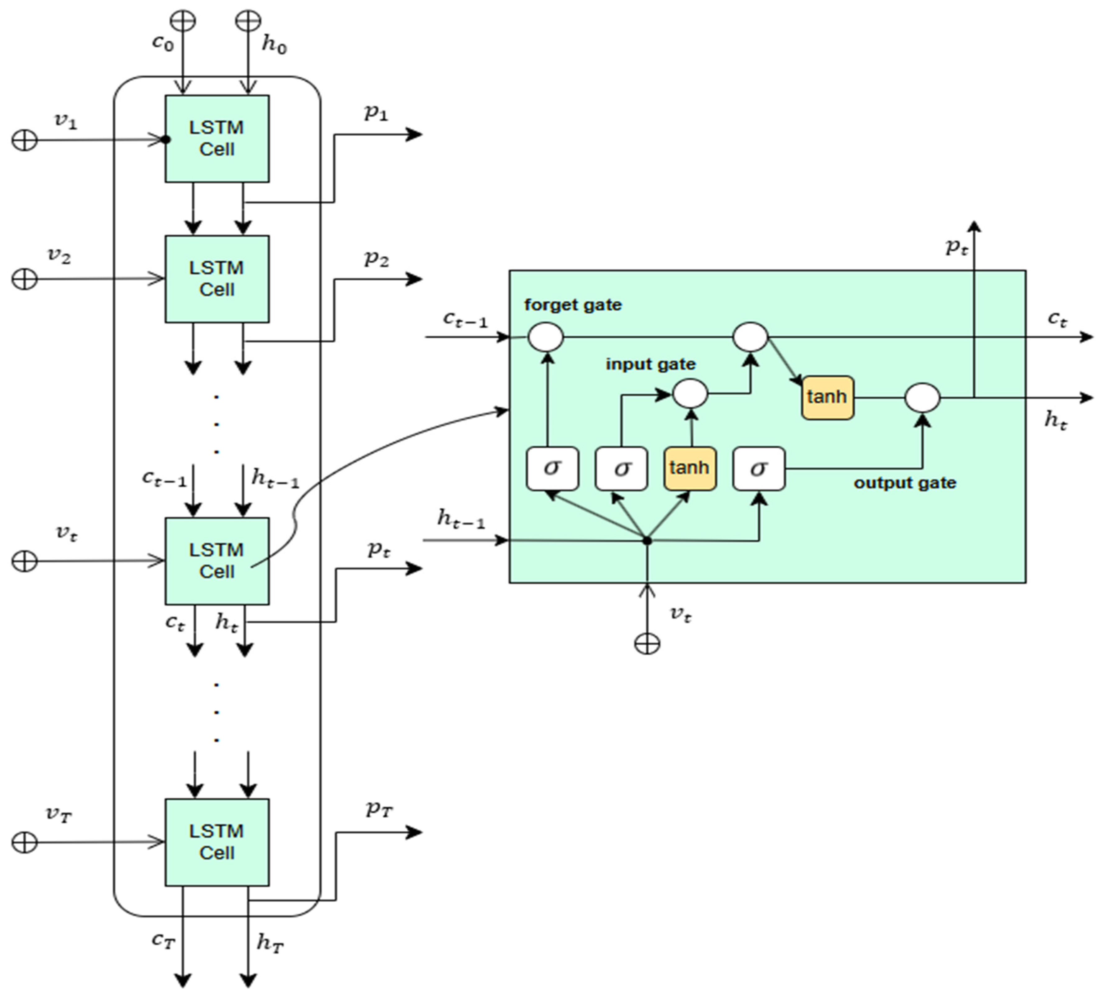
2.2. Long Short-Term Memory

LSTM is a type of artificial neural network architecture specifically designed for time series data and sequential data modeling [55]. LSTM addresses one of the fundamental problems faced by traditional recurrent neural networks (RNNs), known as the “vanishing gradient” problem, and provides the ability to store and retrieve information over long time intervals. This capability of LSTM to store, process, and recall information over extended periods makes it highly effective in modeling complex relationships in sequential data.
The LSTM architecture differs from that of traditional RNNs by incorporating specialized memory cells and gate mechanisms that control access to these cells. Through the input gate, forget gate, and output gate, the model dynamically determines when to take in, store, and output information [56]. These mechanisms also enable the model to filter out unnecessary information while learning long-term dependencies. In LSTM networks, memory management is facilitated by a structure called the cell state, which is effectively controlled through the gates.
The architecture of an LSTM layer with T time steps and the structure of an LSTM cell is illustrated in Figure 1, where the input time series data are denoted as v = v 1 , v 2 , , v t , , v T , and the output values are represented as p = p 1 , p 2 , , p t , , p T .
In Figure 1, h t represents the output, also referred to as the hidden state, while c t denotes the cell state at time step t . A standard LSTM cell consists of sigmoid ( σ ) and hyperbolic tangent activation functions (tanh), along with pointwise addition ( + ) and multiplication ( ) operations. By updating the gates on the memory cell c t —namely, the input gate ( i t ) , forget gate ( f t ) , and output gate ( p t ) —the LSTM can predict the target variables p = p 1 , p 2 , , p t , , p T . In an LSTM layer, the learnable weights are divided into three groups: input weights ( W ), recurrent weights ( R ), and bias ( b ). These matrices represent the concatenated input weights, recurrent weights, and bias values for each component. The layer combines these matrices according to the following equations.
W = W i W f W p W c R = R i R f R p R c   b = b i b f b p b c
In this context, the mathematical formulation of the LSTM is described below:
i t = σ W i v t + R i h t 1 + b i
f t = σ W f v t + R f h t 1 + b f
p t = σ W p v t + R p h t 1 + b p
c t = f t c t 1 + i t c ~ t
c ~ t = σ W c v t + R c h t 1 + b c
h t = v t σ c t
where c t 1 and h t 1 are, respectively, the previous cell state and its output vector, and h t is the output vector.

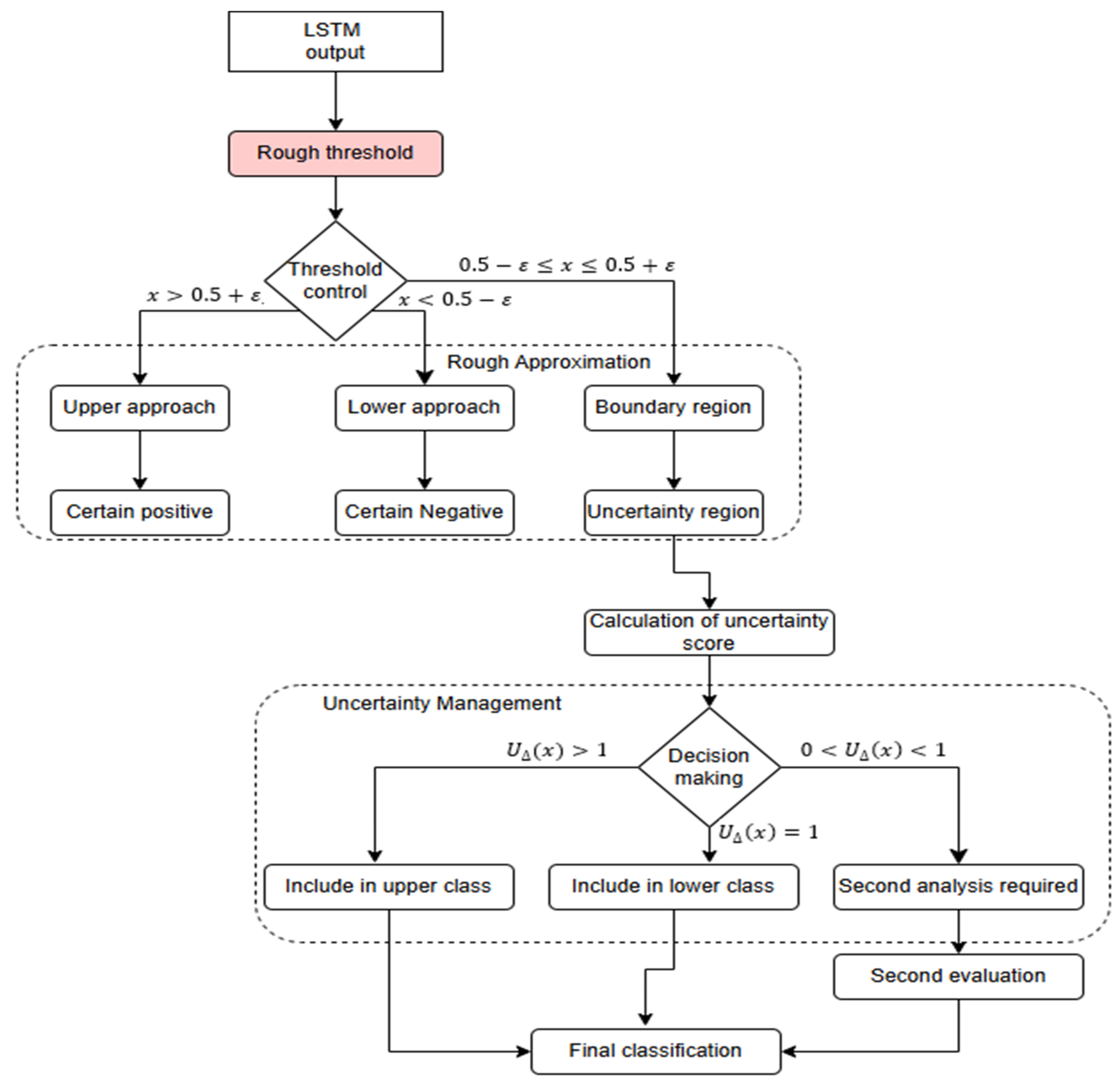
3. Proposed Model: RoughLSTM

In this study, a novel approach called RoughLSTM is proposed. This method integrates the LSTM model, commonly used in time series data analysis, with RST in order to overcome the limitations of LSTM and obtain more reliable results, particularly for complex problems such as anomaly detection. Although LSTM has shown considerable success in time series analysis, it generates outputs based on exact classification thresholds, which may lead to false positive or false negative results, especially when dealing with uncertain or ambiguous data. Rough set theory, on the other hand, models these uncertainties explicitly, offering a more flexible approach to the classification process. RoughLSTM combines the strengths of LSTM in time series analysis with the uncertainty management capabilities of RST. This enables a clearer distinction between the regions of certain and uncertain classes. The proposed architecture begins with a preprocessing phase that includes normalization, windowing with a size of 50, and data augmentation for time series inputs. The core structure consists of two LSTM layers with 100 and 50 units, respectively, separated by dropout layers to prevent overfitting. The model incorporates two fully connected layers—an initial layer with two units and a final layer with thirty units—utilizing ReLU activation functions throughout and Softmax activation in the output layer. A key feature of this architecture is the rough set layer with an epsilon value of 0.1, which processes the outputs to classify signals as either normal or anomalous. In particular, handling examples in boundary regions more accurately enhances the overall accuracy of the model and allows for more reliable classification of uncertain data. The working mechanism of the proposed RoughLSTM model is schematically illustrated in Figure 2. This diagram presents the data flow, components, and processing steps of the model in detail. Additionally, the internal functioning of the rough set layer in the RoughLSTM model is explained in detail, and an operational diagram is provided in Figure 3 to visualize this process.
In this study, RST is used to process the outputs of the LSTM model. The LSTM model processes the time series data and generates an output value for each time step. These output values are typically expressed as a probability score (e.g., in the range of [0, 1]). However, classifying these scores based on an exact threshold value (e.g., 0.5) may result in incorrect outcomes for ambiguous examples. To address this issue, an uncertainty threshold (ε) is introduced, which is determined heuristically based on the distribution of model outputs. The selection of ε is guided by empirical analysis, ensuring that the boundary region effectively captures ambiguous cases while maintaining a balance between false positives and false negatives. This threshold is optimized according to the data distribution and determines the precision of the model. In this context, the uncertainty region ( u r ) is defined as follows:
u r = 0.5 ε ,   0.5 + ε
In the formula, 0.5 indicates the decision boundary in the classification problem. Moreover, this stage divides the outputs of the model into three main regions: the upper approach, lower approach, and border region.
Upper approach ( r R ¯ ): The samples in this region definitively belong to a specific class. The mathematical expression for this region is as follows:
r R ¯ x = x x > 0.5 + ε
Definite positive samples, i.e., those with values greater than 0.5 + ε , are considered anomalies with high confidence. These are the most reliable and accurately detected anomaly samples by the model.
Lower approach ( r R _ ): This includes definitive negative samples. Mathematically, it is expressed as follows:
r R _ x = x x < 0.5 ε
Definite negative samples, i.e., those with values less than 0.5 − ε, are classified as normal cases with high confidence. This region represents the samples that the model confidently identifies as normal.
Boundary region ( r R r ): The boundary region contains ambiguous samples. The samples in this region require further analysis and are defined as follows:
r R r x = x   0.5 ε x 0.5 + ε
Ambiguous samples, where the data fall between 0.5 − ε and 0.5 + ε, are cases that require further analysis. This region represents situations where the model needs additional information or secondary evaluations.
In the next step, the uncertainty score is calculated. For each ambiguous sample, an uncertainty score is calculated based on its distance from the boundary region. This score is then normalized to a standard value.
U ( x ) = | x 0.5 | ε
where x represents the output value of the model. Once the uncertainty score is determined, the decision mechanism classifies samples based on their uncertainty levels:
High-score samples ( U ( x ) > 1 ): These samples are far from the boundary region, making them highly reliable for classification.
  • If x > 0.5 + ε , the sample is classified as an anomaly with high confidence.
  • If x < 0.5 ε , the sample is classified as normal with high confidence.
Low-score samples ( U x = 1 ): These samples lie exactly on the boundary of the uncertainty region. They can still be classified using the standard threshold-based approach but may require additional verification.
Medium-score samples ( 0 < U x < 1 ): These samples fall within the uncertainty region and require further analysis before making a final decision. A secondary analysis can involve additional contextual information, feature extraction, or ensemble-based decision-making to improve classification reliability.
By incorporating this adaptive decision mechanism, RoughLSTM effectively mitigates the limitations of sharp classification boundaries in standard LSTM models. This approach enhances the robustness of anomaly detection by reducing false positives and false negatives, improving interpretability, and allowing for a more flexible decision-making process in uncertain cases.
The step-by-step operation of the RoughLSTM model is detailed in the pseudocode provided in Algorithm 1. This pseudocode clearly outlines the key components of the model, including data input, handling of uncertainties in the rough set layer, and time series analysis performed by the LSTM network. Thus, the implementation and workflow of the RoughLSTM model are systematically presented.
Algorithm 1 RoughLSTM Pseudocode
1: procedure RoughLSTM(signal, num samples, anomaly intervals)
2: Convert signal to double if necessary
3: Normalize signal
                      ▷ Windowing the Signal
4: Define window size = 50, overlap = 25
5: Compute num windows
6: for i = 1 to num windows do
7: Extract window from signal
8: Check if window overlaps with any anomaly intervals
9: Label as normal (1) or anomalous (0)
10: end for
                      ▷ Rough Set Parameters
11: Define ϵ = 0.1 (uncertainty threshold)
12: Generate additional noisy samples
                      ▷ Convert Data to LSTM Format
13: Store augmented data
14: Convert each window to cell array format
                      ▷ Train-Test Split
15: Shuffle data
16: Split into Train (70%), Validation (15%), and Test (15%)
                      ▷ Convert Labels to Categorical
17: Convert 0 (Anomalous) and 1 (Normal) to categorical format
                      ▷ Define Rough-LSTM Model
18: Define network layers (LSTM, Dropout, Rough Set Layer, Fully Con- nected)
                      ▷ Train the Model
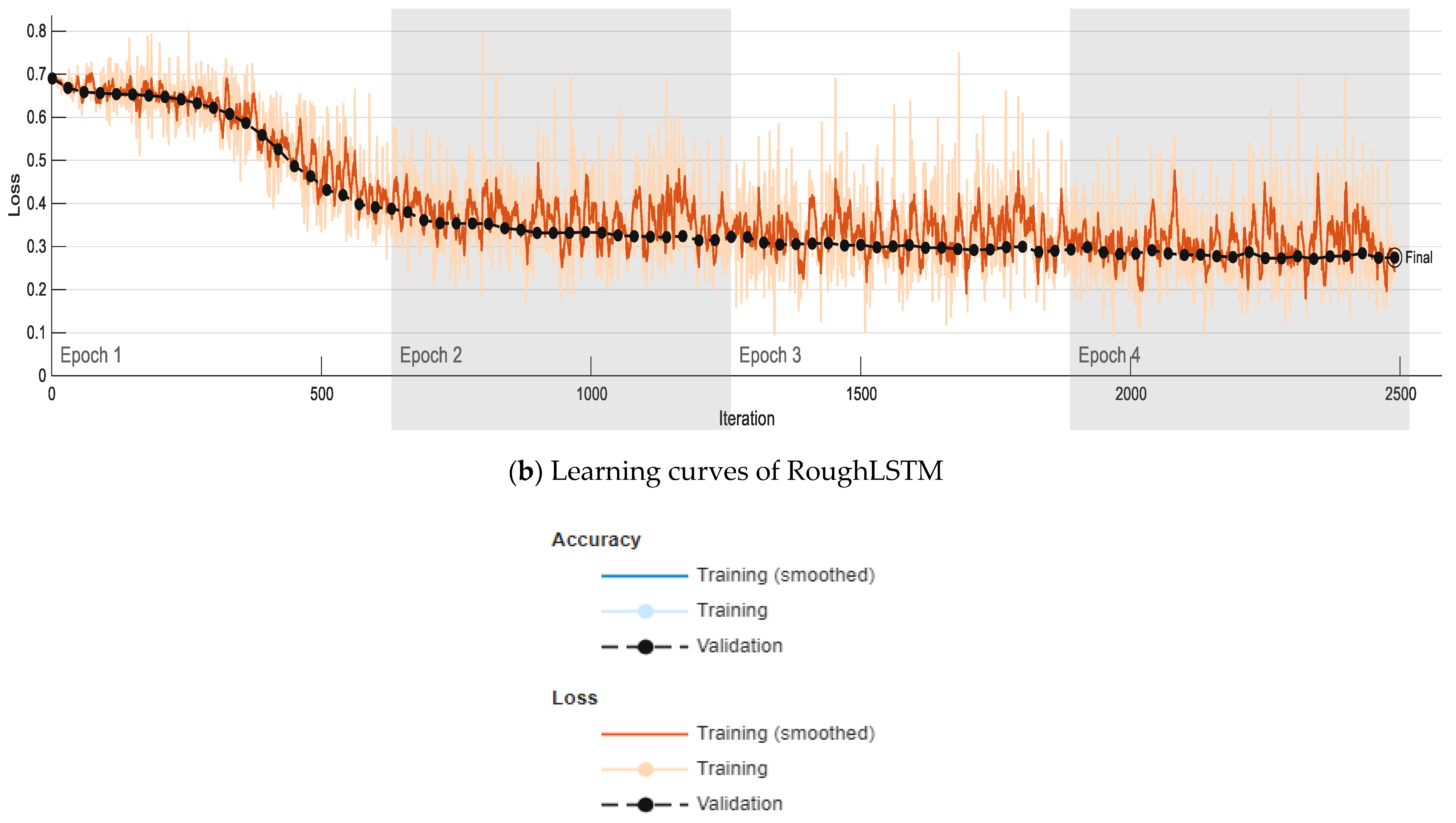
19: Train using Adam optimizer with 50 epochs
                      ▷ Testing and Post-processing
20: Predict using trained model
21: Apply Rough Set Post-processin
                      ▷ Compute Accuracy
22: Compare predictions with ground truth
23: Compute accuracy
24: return Y PredRoughLSTM, accuracyRoughLSTM
25: end procedure

4. Experimental Results and Discussion
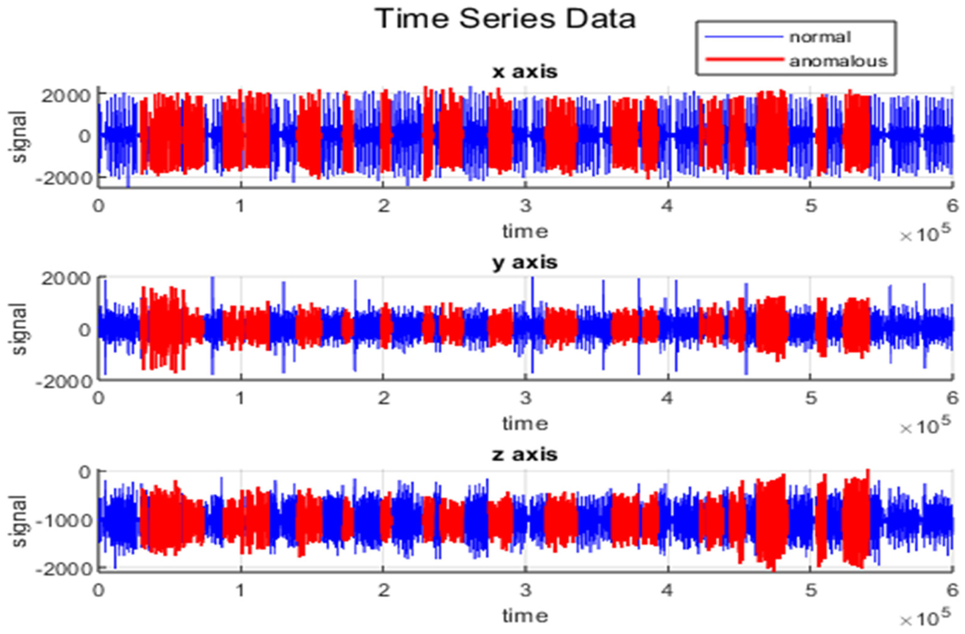
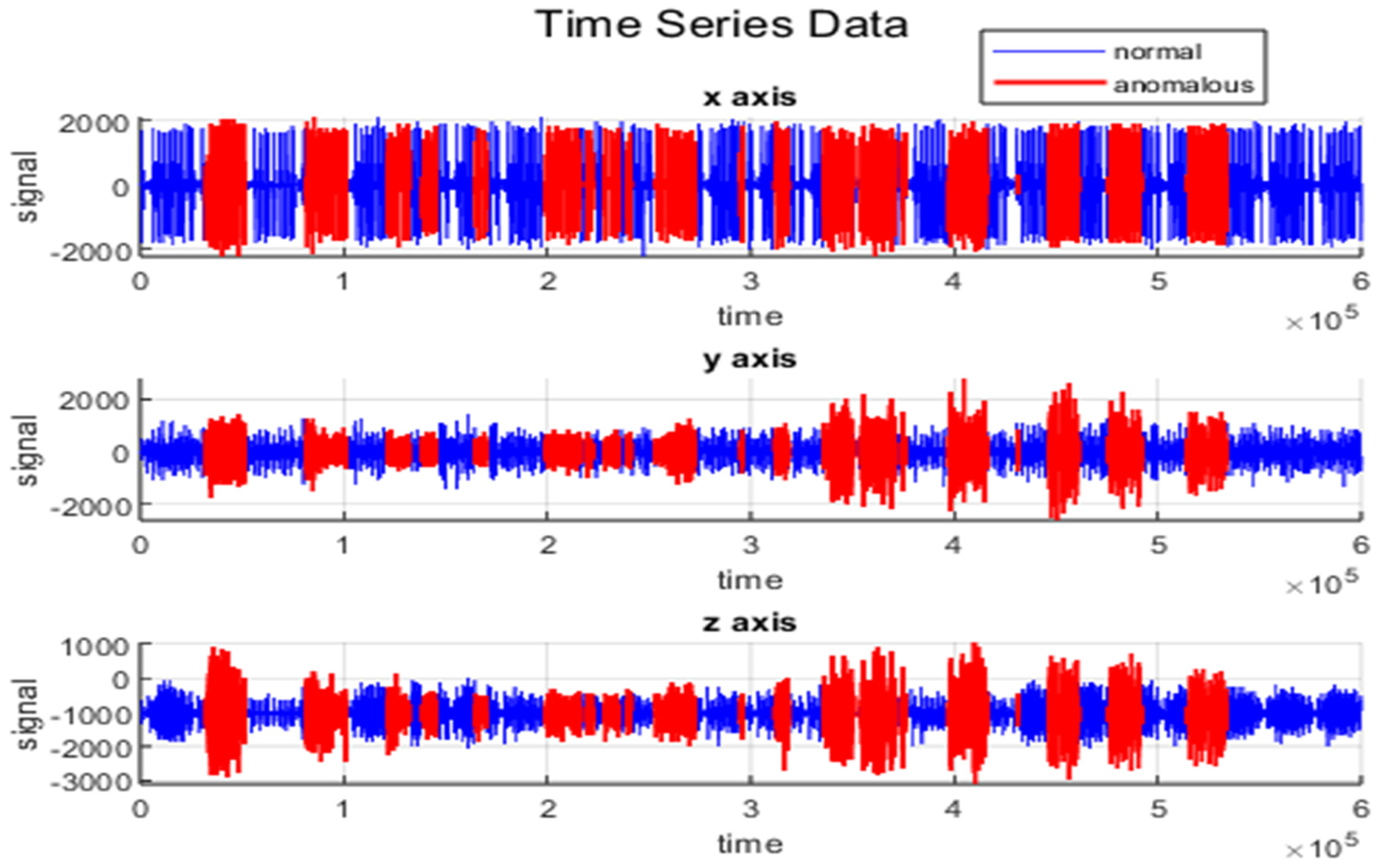
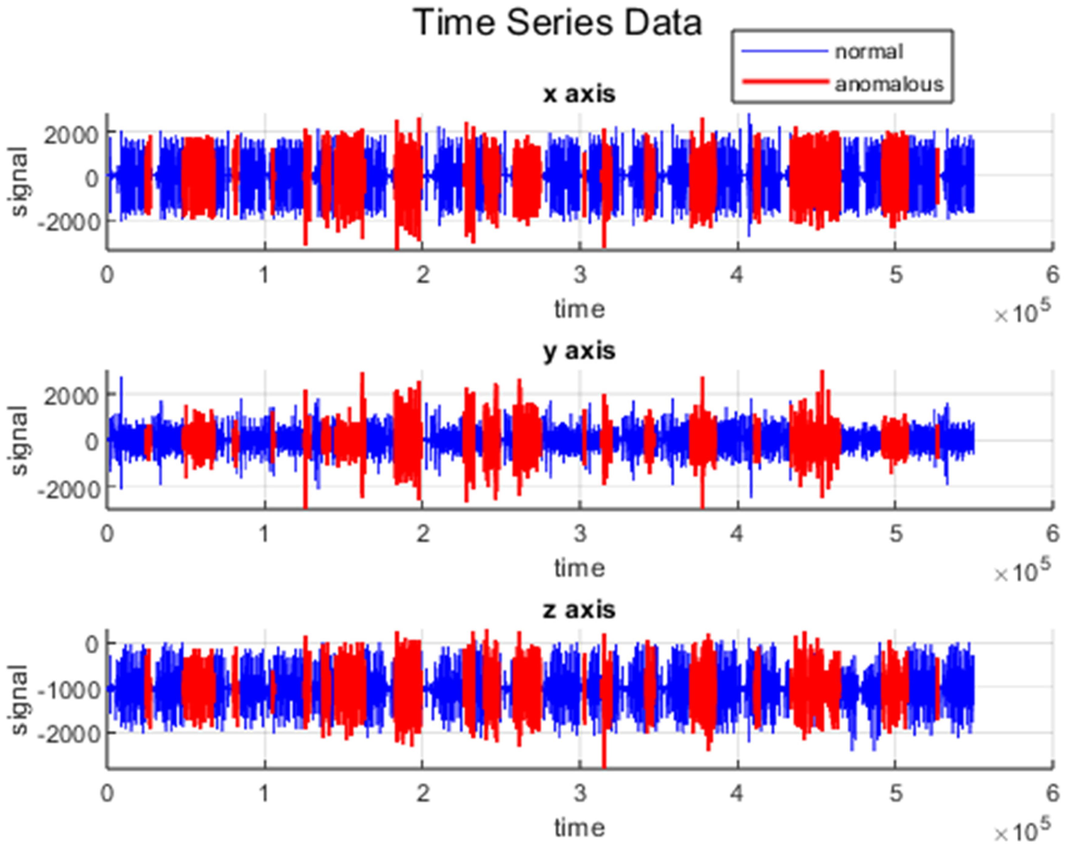
In this section, the dataset used is first described, followed by an explanation of the performance evaluation metrics, and finally, the performance analysis of the models is conducted.

4.1. Dataset

The dataset presented in this study is a comprehensive collection of vibration data acquired from CNC milling machines in a real-world production environment. The data were collected over a two-year period (October 2018 to August 2021) from three different CNC machines (M01, M02, and M03) operating in a production plant [57]. The dataset is designed to address the challenges of industrial machine learning applications, particularly in the context of process monitoring and anomaly detection. The dataset consists of vibration data collected during various tool operations (OPs) performed by the CNC machines. Each operation represents a specific machining process with unique parameters, such as spindle speed, feed rate, and duration. The dataset includes 15 different tool operations, each characterized by its own set of parameters, as summarized in Table 1.
Tool operations: Each operation (OP00 to OP14) is defined by its spindle speed (RPM), feed rate (mm/s), and duration (seconds). For example, OP00 is a step drill operation with a spindle speed of 250 RPM, a feed rate of 100 mm/s, and a duration of 132 s.
Data segmentation: The raw vibration data were manually segmented into individual tool operations. Each segment corresponds to a specific operation performed by the machine. The dataset includes labeled data, where each tool operation is annotated as either “OK” (normal) or “NOK” (abnormal). The annotations were provided by production experts based on the quality control checks performed after each batch of workpieces. The abnormal cases (NOK) include process failures such as tool breakage, improper tool clamping, and chip jamming [57].

4.2. Evaluation Metrics

A confusion matrix is a performance evaluation table used for classification models. It summarizes the number of correct and incorrect predictions across different classes, providing insights into model performance. The structure of the confusion matrix is presented in Table 2.
Accuracy is a measure of the proportion of instances that are correctly classified [58]. Mathematically expressed:
A c c u r a c y = T P + T N T P + T N + F P + F N
The receiver operating characteristic (ROC) curve is a graphical representation used to evaluate the performance of a classification model, especially in binary classification problems. It plots the true positive rate (TPR) against the false positive rate (FPR) at various threshold levels, showing the trade-off between sensitivity and specificity.
TPR: Measures how well the model correctly identifies positive instances. Mathematical expression:
T P R = T P T P + F N
FPR: Measures the proportion of negative instances that are incorrectly classified as positive. Mathematical expression:
F P R = F P F P + T N

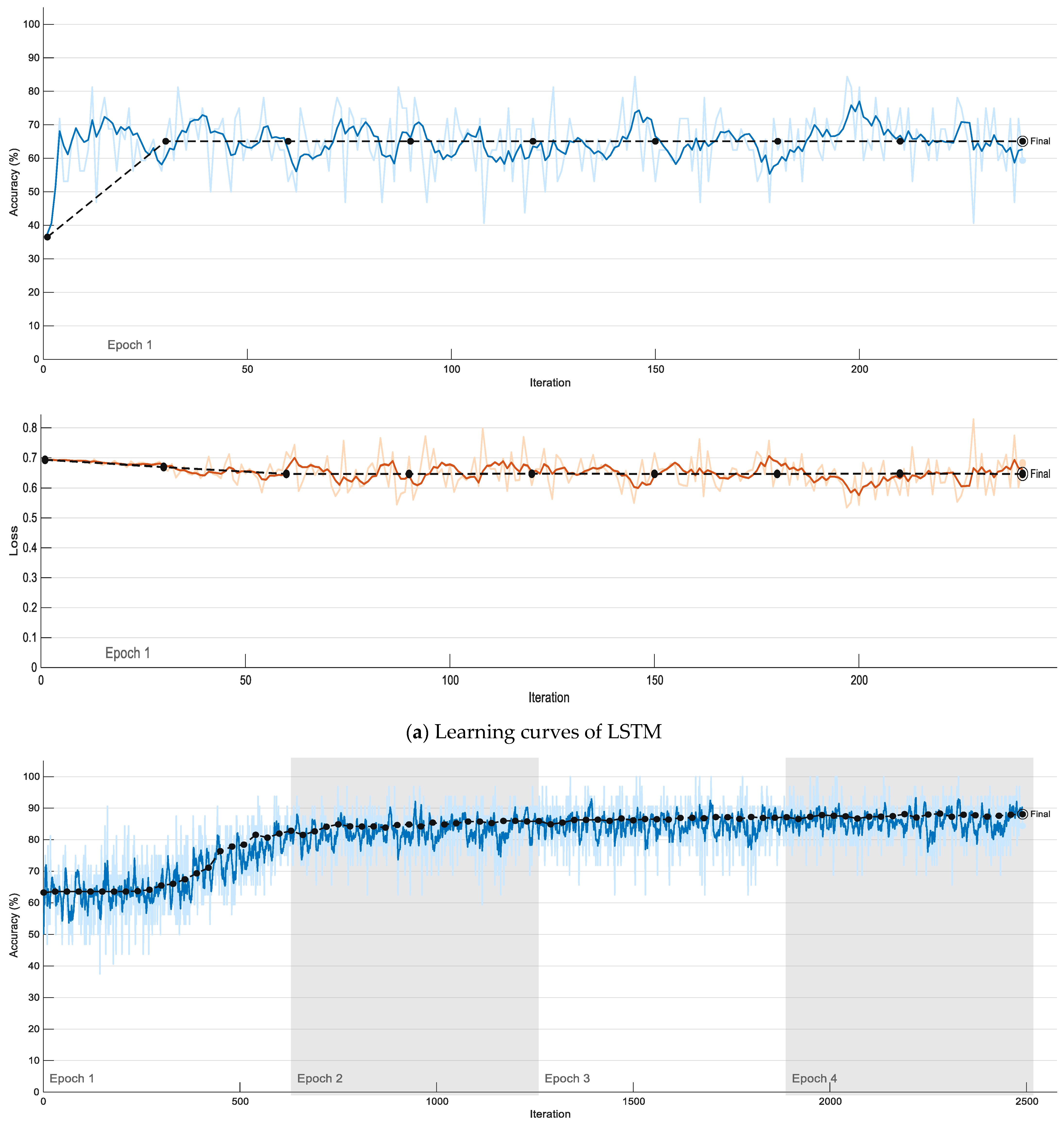
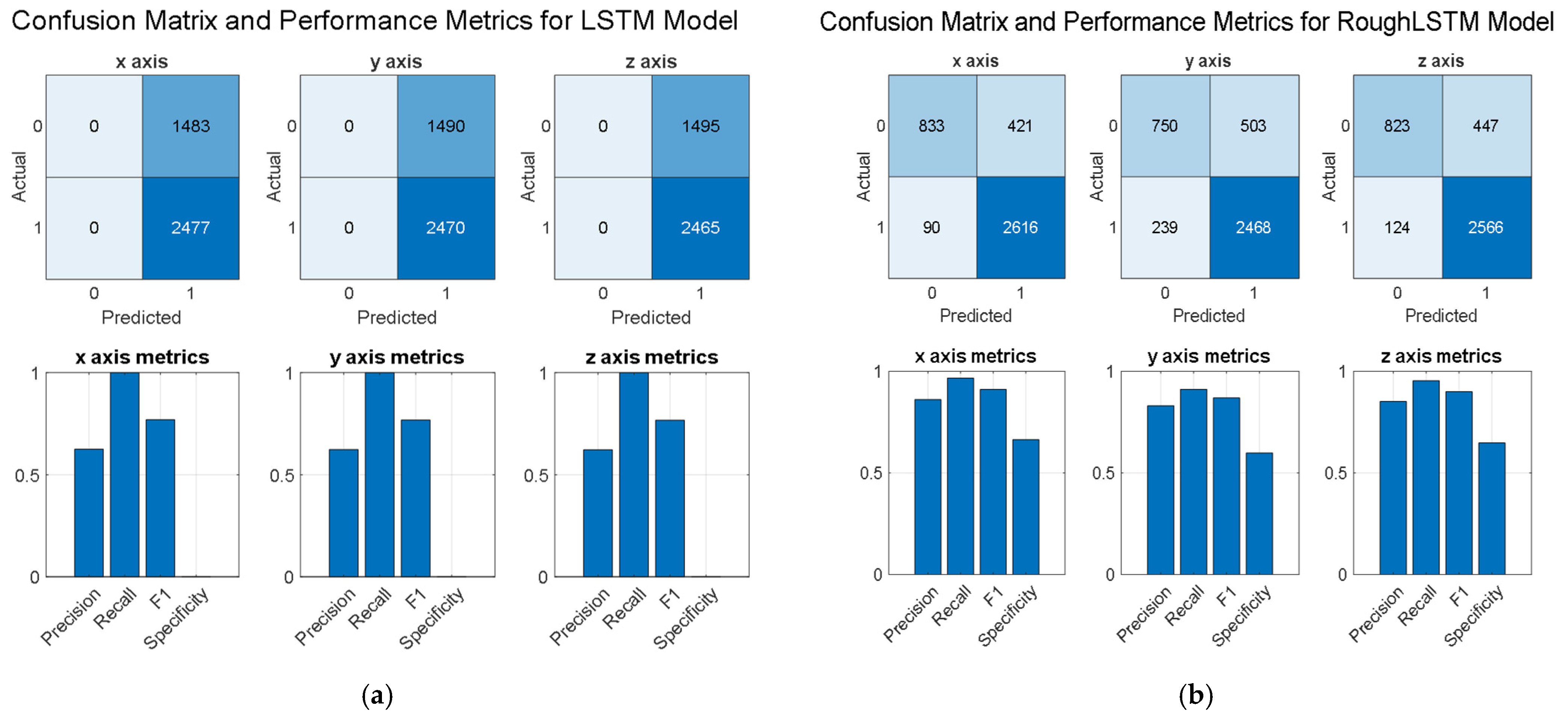
4.3. Performance Analysis

This section presents a comprehensive performance analysis of the proposed RoughLSTM model, compared with the conventional LSTM model. In this study, anomaly detection was conducted using vibration data obtained from industrial CNC machines. The dataset consists of vibration data collected under real production conditions from three different CNC machines (MO1, MO2, and MO3) over a two-year period. The experimental studies were conducted on both RoughLSTM and LSTM models based on predefined hyperparameters. The performance of these models was evaluated using key metrics such as accuracy, loss, and the ROC curve. The primary objective of these experiments is to demonstrate the effectiveness of RoughLSTM in anomaly detection compared to the conventional LSTM model and to assess its applicability in industrial settings.
Within the scope of the experimental analysis, different operational scenarios were considered. Initially, four different operation (option) scenarios were randomly selected for each CNC machine. For instance, for the M01 machine, vibration data from OP02, OP05, OP08, OP11, and OP14 operations were combined to conduct anomaly detection analysis. The performance metrics obtained from these analyses are presented in the form of tables and graphical representations. In addition, the vibration data of OP02, OP05, OP08, OP11, and OP14 operations of the M01 machine are shown in Figure 4.
Figure 4 visually presents the temporal behavior of vibration data measured during different operations, along with potential anomalous signals. The performance of the models on this time series is analyzed in detail based on various metrics, including accuracy–loss, confusion matrix, and the ROC curve, which are respectively illustrated in Figure 5, Figure 6 and Figure 7.
Panels (a) and (b) in Figure 5 show the learning curves of the LSTM and RoughLSTM models, respectively. In the figure, training and validation processes are analyzed through accuracy and loss metrics.
In Figure 5, examining the learning curves of LSTM and RoughLSTM models, significant performance differences are observed between the two models. The learning curve of the LSTM model (Figure 5a) shows rapid accuracy improvement within approximately 200 iterations (1 epoch) before stabilizing. This quick convergence indicates early learning by the model but suggests it remains at a lower accuracy level. Although the loss value in the LSTM model decreases over time, the observed fluctuations indicate that the model carries a risk of overfitting and has not reached sufficient learning capacity. While the LSTM model, which shows high variance initially, becomes relatively stable after certain iterations, the fluctuations in validation accuracy indicate that the model struggles to generalize to test data.
In contrast, the learning curve of the RoughLSTM model (Figure 5b) shows continuous improvement over approximately 2500 iterations (4 epochs). This extended learning period proves that the model absorbs more information and demonstrates better generalization. The accuracy values of the RoughLSTM model show more stable improvement throughout the training process compared to LSTM and exhibit fewer fluctuations. The model’s rapid adaptation ability is particularly noteworthy in the shaded areas (Epochs 2, 3, and 4). The rapid decrease in training loss and controlled decline in validation loss demonstrate that the RoughLSTM model learns more efficiently and exhibits stronger generalization performance. The steady progression of validation accuracy indicates that the model can produce more reliable results in practical applications.
When Table 3 is examined, RoughLSTM is seen to outperform LSTM in training and validation by about 4–6%. This difference indicates that the generalization ability of the model is stronger. RoughLSTM offers lower losses in both the training and validation phase. A lower validation loss indicates that the model is less likely to be overfitting. RoughLSTM shows lower variance than LSTM, which proves that the model offers more stable learning.
In Figure 6, examining the confusion matrices and performance metrics of both models across three axes (x, y, z), significant differences are revealed. The LSTM model (Figure 6a) shows extreme overfitting to class “1” across all axes (x, y, z) and misclassifies all examples belonging to class “0” as false negatives. It incorrectly classifies 2281 samples on the x-axis, 2284 on the y-axis, and 2290 on the z-axis as false positives. This indicates that the model failed to achieve balanced learning and is biased towards a single class. Additionally, the precision, recall, and specificity metrics for the LSTM model reflect this imbalance, with recall values being notably high due to the model’s bias toward class “1” but specificity being considerably low. In contrast, the RoughLSTM model (Figure 6b) demonstrates more balanced classification performance. On the x-axis, it achieves 1105 true negatives and 2118 true positives, while on the y-axis, it shows 1181 true negatives and 2096 true positives. The z-axis performance reveals 1462 true negatives and 2222 true positives, the model successfully making reasonable predictions for both classes. Unlike the LSTM model, RoughLSTM does not suffer from extreme class bias, as seen in the more evenly distributed precision, recall, and specificity values. The additional performance metrics (precision, recall, F1-score, and specificity) further validate RoughLSTM’s superiority. While the LSTM model achieves high recall due to class bias, RoughLSTM maintains a better trade-off between precision and recall, ensuring that both classes are correctly identified. The specificity scores also confirm RoughLSTM’s ability to avoid misclassifications of negative cases, which is crucial for real-world anomaly detection applications.
In conclusion, the RoughLSTM model shows a more balanced and reliable classification performance. Unlike the LSTM model, it can recognize both classes and has a lower misclassification rate. This indicates that RoughLSTM is more suitable for practical applications. The model’s ability to maintain good performance across all axes while correctly identifying both positive and negative cases demonstrates its superior generalization capability and robustness compared to the standard LSTM model.
Figure 7 compares the ROC curves and AUC distributions of the LSTM model and the RoughLSTM model. In Figure 7a, the ROC curve of the LSTM model nearly follows the 45-degree line (random guess line), with AUC (area under the curve) values of 0.503, 0.507, and 0.493, respectively. These values indicate that the model’s classification performance is at the level of random guessing, making it ineffective for this dataset. Additionally, the AUC distributions at the bottom further confirm the model’s poor performance, as the bootstrap distributions are tightly clustered around 0.50, reinforcing its lack of discriminative power. Conversely, Figure 7b demonstrates that the RoughLSTM model significantly improves classification performance. The ROC curves for the x, y, and z axes are much closer to the upper-left corner, resembling an ideal classifier. The AUC values of 0.935, 0.959, and 0.979 indicate that the RoughLSTM model effectively differentiates between the two classes. Furthermore, the AUC distributions show a clear separation from the random guessing threshold, with mean AUC values consistently above 0.93 and well-defined confidence intervals. These findings strongly confirm that RoughLSTM significantly outperforms the standard LSTM model, providing a robust and reliable classification approach for this dataset.
Table 4 presents the cross-validation metrics for the LSTM and RoughLSTM models using different operations (OP02, OP05, OP08, OP11, OP14) of the M01 machine. The table is divided into two sections: (a) for the LSTM model and (b) for the RoughLSTM model. (a) LSTM model: The performance metrics for this model are generally low. The AUC values range between 0.503 and 0.507, and the F1-scores are between 0.731 and 0.733. Although the recall values are 1.000, the specificity values are 0.000, indicating that the model fails to correctly identify negative classes. (b) RoughLSTM model: This model shows significantly better performance compared to LSTM. The AUC values range from 0.929 to 0.979, and the F1-scores are between 0.852 and 0.942. The recall and specificity values are more balanced and higher, indicating that the model better identifies both positive and negative classes.
In this section, as the next step, the experimental studies conducted for the M01 machine were similarly applied to the M02 and M03 machines. However, at this stage, only the confusion matrix and ROC values are presented, instead of the learning curves of the methods.
Figure 8 shows an example of the combination of vibration data obtained in OP00, OP01, OP04, OP07, and OP09 operations on the MO2 machine.
In the confusion matrices (See Figure 9) for the LSTM model, the false negative (FN) rates are significantly high, indicating that the model fails to distinguish between classes and misclassifies almost all instances. This poor performance is evident across the x, y, and z axes, where the model predicts almost all instances incorrectly. In contrast, the RoughLSTM model reduces false negatives and false positives considerably, leading to a significant increase in correct predictions. This improvement is clearly visible in the confusion matrices, where the RoughLSTM model demonstrates a better balance between actual and predicted values. Additionally, the F1-scores in Figure 9 highlight another critical difference between the models. The LSTM model has low precision and recall values, leading to poor F1-scores, which confirm its inability to correctly identify class instances. However, the RoughLSTM model achieves substantially higher F1-scores, reinforcing its ability to balance precision and recall effectively. This suggests that RoughLSTM not only improves classification accuracy but also ensures better overall model robustness. In Figure 10, examining the ROC curves, the LSTM model’s curve follows the random guess line, with AUC values (0.495, 0.493, 0.493) being very low, confirming its inefficiency. On the other hand, the RoughLSTM model’s ROC curves are closer to the upper-left corner, achieving AUC values of 0.845, 0.952, and 0.895, which indicate strong classification performance.
Table 5 compares the performance of the LSTM and RoughLSTM models on the M03 machine. LSTM (a) shows low performance, while RoughLSTM (b) delivers higher and more balanced metrics. RoughLSTM particularly excels in AUC and F1-score.
Overall, the RoughLSTM model significantly outperforms the LSTM model, greatly improving classification accuracy. These results demonstrate that RoughLSTM is a more reliable model, particularly showing superior performance along the y and z axes.
Similarly, the vibration data for operations OP01, OP02, OP04, OP07, and OP10 of the M03 machine are presented in Figure 11, while the results obtained for the methods are shown in Figure 12 and Figure 13.
Table 6 compares the LSTM and RoughLSTM models on the M03 machine. LSTM (a) shows low AUC (0.489–0.512) and zero specificity despite perfect recall, indicating poor negative class identification. RoughLSTM (b) performs significantly better, with higher AUC (0.912–0.943), balanced recall–specificity, and improved F1-scores (0.869–0.911), demonstrating superior overall performance.
In this study, the accuracy values of the LSTM and RoughLSTM models were compared through experiments conducted on MO1, MO2, and MO3 machines, and the results are given in Table 7. The results indicate that RoughLSTM achieved higher accuracy across all machines and axes compared to LSTM. While the accuracy of LSTM models generally remained in the 60–70% range, RoughLSTM demonstrated superior performance, ranging from 73% to 90%. When analyzed on a machine basis, RoughLSTM achieved 17%, 18%, and 23% higher accuracy on the x, y, and z axes, respectively, for the MO1 machine. For the MO2 machine, the most significant improvement was observed on the y-axis, where RoughLSTM outperformed LSTM by 24%. For the MO3 machine, RoughLSTM demonstrated a performance advantage of 15–20% over LSTM across all axes, further highlighting its superiority. Additionally, the highest values are indicated in dark color and in all other tables, dark color represents the highest value.

4.4. Comparative Performance Analysis

In this section, the accuracy performance of the proposed RoughLSTM model is compared with other approaches, namely CNN–LSTM [32], WaveletLSTMa [16], and conventional LSTM models. The obtained results are evaluated based on axis-based accuracy values for various operations in MO1, MO2, and MO3 machines. Moreover, the results for each machine are presented in Table 5, Table 6, and Table 7, respectively.
As seen in Table 8, in the experiments conducted on the MO1 machine, RoughLSTM achieved the highest or second-highest accuracy values in many operation and axis combinations. In the OP01+OP02 operation, RoughLSTM provided the best results for the x-axis (0.8425) and z-axis (0.8245), while achieving the second-best performance for the y-axis (0.8312). Similarly, in the OP04+OP10 operation, RoughLSTM achieved the highest accuracy for the y-axis (0.8250) and z-axis (0.8367), while maintaining competitive performance in other axes.
Examining Table 9, the experimental results for the MO2 machine indicate that RoughLSTM stands out in certain operations. In the OP02+OP08 operation, RoughLSTM achieved the highest accuracy for the y-axis (0.9389) and z-axis (0.9514). In the OP07+OP11 operation, RoughLSTM demonstrated the best performance for the z-axis (0.9542) and y-axis (0.9347). These findings highlight the effectiveness of RoughLSTM in specific axes on the MO2 machine.
Table 10 presents the results for the MO3 machine, where RoughLSTM exhibits varying performance across different operations. In the OP04+OP07 operation, RoughLSTM provided the highest accuracy for the x-axis (0.8750) and demonstrated competitive performance for the z-axis (0.8233). In the OP10+OP14 operation, RoughLSTM achieved the highest accuracy for the y-axis (0.8792).
The findings reveal that RoughLSTM outperforms other models in many scenarios. Specifically, RoughLSTM has achieved the highest or second-highest accuracy values in many operations on the z-axis. While the LSTM model generally exhibits the lowest performance, RoughLSTM is found to be competitive with or superior to CNN–LSTM and WaveletLSTMa.
In conclusion, the RoughLSTM model demonstrates consistent accuracy across different operation and axis combinations, making it a viable alternative to existing approaches.

5. Conclusions

This study introduced a novel RoughLSTM model for anomaly detection in CNC machine vibration data by integrating rough set theory with long short-term memory networks. The proposed model addresses the limitations of conventional long short-term memory models, particularly in handling uncertainty and ambiguity in vibration data, by classifying inputs into distinct regions: the upper approach, lower approach, and boundary region. This adaptive decision-making mechanism enhances anomaly detection accuracy and reduces false positives and negatives. The RoughLSTM model was evaluated on real-world vibration data collected from CNC milling machines operating under various conditions. A comparative performance analysis was conducted against other deep-learning-based models, including CNN–LSTM, WaveletLSTMa, and conventional LSTM models. Experimental results demonstrate that RoughLSTM outperforms the conventional LSTM in several key performance metrics:
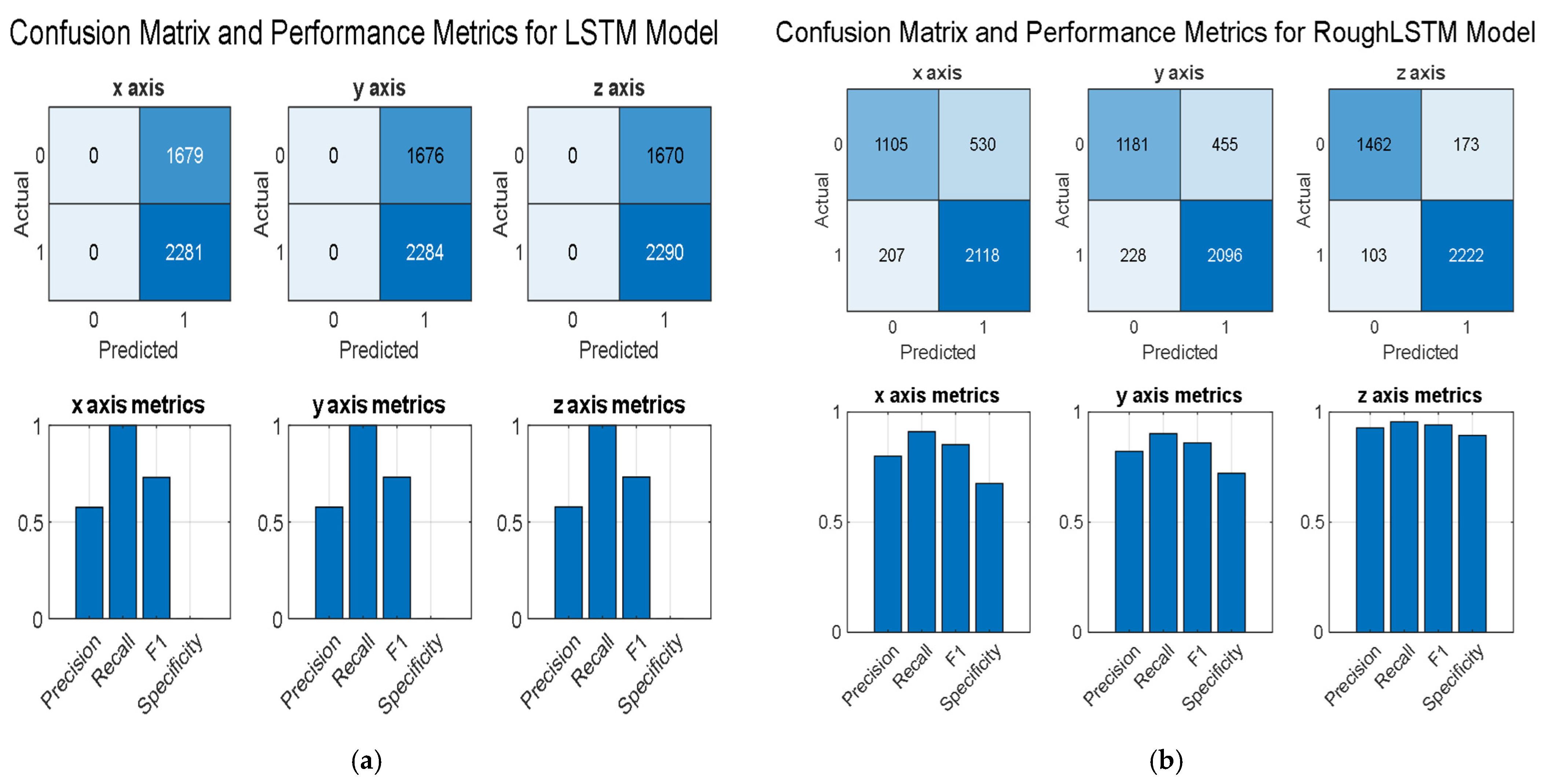
  • Accuracy: RoughLSTM achieved a classification accuracy of 94.3%, compared to 78% for the conventional LSTM.
  • False positive rate (FPR): RoughLSTM reduced the FPR to 3.7%, while the standard LSTM exhibited a much higher rate.
  • False negative rate (FNR): The proposed model minimized the FNR to 2.0%, ensuring reliable detection of anomalies.
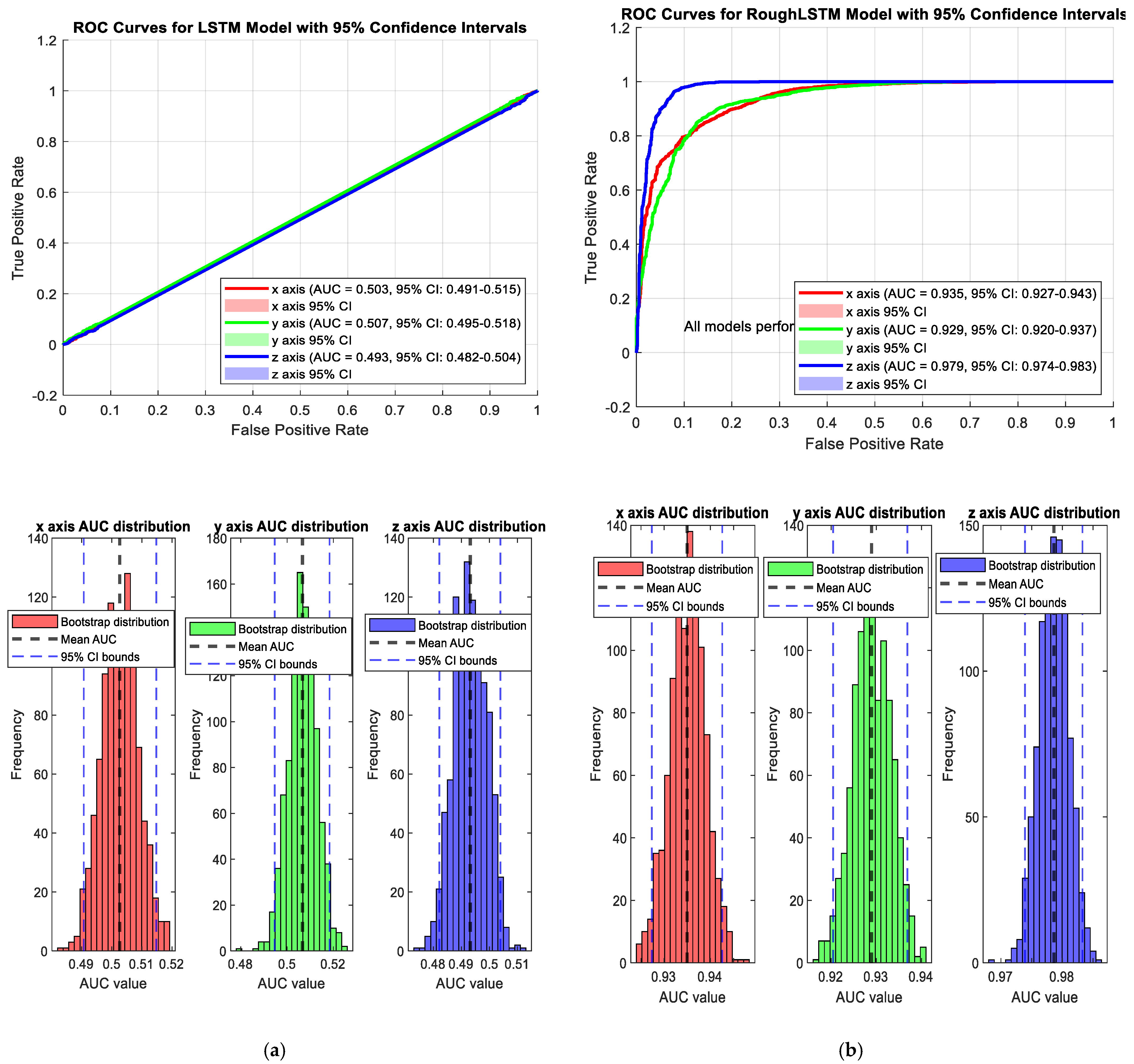
  • AUC (area under the curve): RoughLSTM showed AUC values close to 0.95 across multiple operational scenarios, indicating strong classification performance.
Furthermore, the comparative performance analysis of axis-based accuracy values across MO1, MO2, and MO3 machines confirmed that RoughLSTM consistently delivered superior performance. The model achieved the highest or second-highest accuracy in various operational scenarios, particularly excelling in the z-axis across multiple operations. Compared to CNN–LSTM and WaveletLSTMa, RoughLSTM demonstrated a strong generalization ability, effectively distinguishing between normal and abnormal conditions in complex industrial environments. This performance improvement translates into reduced machine downtime, optimized maintenance schedules, and significant cost savings for industrial operations. The ability of RoughLSTM to provide high-accuracy anomaly detection in different machine settings makes it a robust and scalable solution for predictive maintenance applications.
Future research can explore the integration of additional data sources, such as temperature and acoustic signals, to further enhance anomaly detection accuracy. Moreover, developing real-time implementation of RoughLSTM within an edge computing framework could provide immediate feedback for predictive maintenance systems, further improving industrial process reliability.

Author Contributions

R.Ç.: contributed to the conceptualization and design of the study, developed the methodology, created the software tools, conducted the investigation, and was responsible for writing the original draft of the manuscript. A.T.: led the validation of the study, provided supervision throughout the research, contributed to writing the manuscript with critical reviews, developed the methodology and edits, and managed the overall paper administration. All authors have read and agreed to the published version of the manuscript.

Funding

This research received no external funding.

Data Availability Statement

The Bosch CNC Machining Dataset, which supports this study’s findings, is freely available from the UCI Machine Learning Repository. The dataset is available at https://archive.ics.uci.edu/datasets/?search=CNC, accessed on 10 March 2025.

Conflicts of Interest

The authors declare that they have no known competing financial interests or personal relationships that could have appeared to influence the work reported in this paper.

References

  1. Quatrano, A.; De Simone, M.C.; Rivera, Z.B.; Guida, D. Development and Implementation of a Control System for a Retrofitted CNC Machine by Using Arduino. FME Trans. 2017, 45, 565–571. [Google Scholar] [CrossRef]
  2. Lins, R.G.; Guerreiro, B.; Schmitt, R.; Sun, J.; Corazzim, M.; Silva, F.R. A Novel Methodology for Retrofitting CNC Machines Based on the Context of Industry 4.0. In Proceedings of the 2017 IEEE international systems engineering symposium (ISSE), Vienna, Austria, 11–13 October 2017; IEEE: New York, NY, USA, 2017; pp. 1–6. [Google Scholar]
  3. Yardımeden, A.; Turan, A. Farklı Kesme Parametreleriyle AISI 1040 Çeliğin Tornalanmasında Oluşan Titreşimlerin ve Yüzey Pürüzlülüğün Incelenmesi. Dicle Üniversitesi Mühendislik Fakültesi Mühendislik Derg. 2018, 9, 269–278. [Google Scholar]
  4. Nath, C. Integrated Tool Condition Monitoring Systems and Their Applications: A Comprehensive Review. Procedia Manuf. 2020, 48, 852–863. [Google Scholar] [CrossRef]
  5. Arriaza, O.V.; Tumurkhuyagc, Z.; Kim, D.-W. Chatter Identification Using Multiple Sensors and Multi-Layer Neural Networks. Procedia Manuf. 2018, 17, 150–157. [Google Scholar] [CrossRef]
  6. Yan, S.; Sun, Y. Early Chatter Detection in Thin-Walled Workpiece Milling Process Based on Multi-Synchrosqueezing Transform and Feature Selection. Mech. Syst. Signal Process. 2022, 169, 108622. [Google Scholar] [CrossRef]
  7. Fourlas, G.K.; Karras, G.C. A Survey on Fault Diagnosis and Fault-Tolerant Control Methods for Unmanned Aerial Vehicles. Machines 2021, 9, 197. [Google Scholar] [CrossRef]
  8. Park, J.; Jung, Y.; Kim, J.-H. Multiclass Classification Fault Diagnosis of Multirotor UAVs Utilizing a Deep Neural Network. Int. J. Control. Autom. Syst. 2022, 20, 1316–1326. [Google Scholar] [CrossRef]
  9. Zhang, X.; Zhao, Z.; Wang, Z.; Wang, X. Fault Detection and Identification Method for Quadcopter Based on Airframe Vibration Signals. Sensors 2021, 21, 581. [Google Scholar] [CrossRef]
  10. Altinors, A.; Yol, F.; Yaman, O. A Sound Based Method for Fault Detection with Statistical Feature Extraction in UAV Motors. Appl. Acoust. 2021, 183, 108325. [Google Scholar] [CrossRef]
  11. Han, Y.; Qi, Z.; Tian, Y. Anomaly Classification Based on Self-Supervised Learning and Its Application. J. Radiat. Res. Appl. Sci. 2024, 17, 100918. [Google Scholar] [CrossRef]
  12. Darban, Z.Z.; Webb, G.I.; Pan, S.; Aggarwal, C.C.; Salehi, M. CARLA: Self-Supervised Contrastive Representation Learning for Time Series Anomaly Detection. Pattern Recognit. 2025, 157, 110874. [Google Scholar] [CrossRef]
  13. Fatemifar, S.; Awais, M.; Akbari, A.; Kittler, J. Pure Anomaly Detection via Self-Supervised Deep Metric Learning with Adaptive Margin. Neurocomputing 2025, 611, 128659. [Google Scholar] [CrossRef]
  14. Han, H.; Fan, H.; Huang, X.; Han, C. Self-Supervised Multi-Transformation Learning for Time Series Anomaly Detection. Expert. Syst. Appl. 2024, 253, 124339. [Google Scholar] [CrossRef]
  15. Choubey, M.; Chaurasiya, R.K.; Yadav, J.S. Contrastive Learning for Efficient Anomaly Detection in Electricity Load Data. Sustain. Energy Grids Netw. 2025, 42, 101639. [Google Scholar] [CrossRef]
  16. Fadi, O.; Bahaj, A.; Zkik, K.; El Ghazi, A.; Ghogho, M.; Boulmalf, M. Smart Contract Anomaly Detection: The Contrastive Learning Paradigm. Comput. Netw. 2025, 260, 111121. [Google Scholar] [CrossRef]
  17. Chi, J.; Mao, Z. One-Classification Anomaly Detection: Utilizing Contrastive Transfer Learning. Measurement 2025, 242, 116173. [Google Scholar] [CrossRef]
  18. Xiao, B.W.; Xing, H.J.; Li, C.G. MulGad: Multi-Granularity Contrastive Learning for Multivariate Time Series Anomaly Detection. Inf. Fusion. 2025, 119, 103008. [Google Scholar] [CrossRef]
  19. Kang, H.; Kang, P. Transformer-Based Multivariate Time Series Anomaly Detection Using Inter-Variable Attention Mechanism. Knowl. Based Syst. 2024, 290, 111507. [Google Scholar] [CrossRef]
  20. Gao, R.; Wang, J.; Yu, Y.; Wu, J.; Zhang, L. Enhanced Graph Diffusion Learning with Dynamic Transformer for Anomaly Detection in Multivariate Time Series. Neurocomputing 2025, 619, 129168. [Google Scholar] [CrossRef]
  21. Sui, L.; Jiang, Y. Argo Data Anomaly Detection Based on Transformer and Fourier Transform. J. Sea Res. 2024, 198, 102483. [Google Scholar] [CrossRef]
  22. LeCun, Y.; Bengio, Y.; Hinton, G. Deep Learning. Nature 2015, 521, 436–444. [Google Scholar] [CrossRef] [PubMed]
  23. Glaeser, A.; Selvaraj, V.; Lee, S.; Hwang, Y.; Lee, K.; Lee, N.; Lee, S.; Min, S. Applications of Deep Learning for Fault Detection in Industrial Cold Forging. Int. J. Prod. Res. 2021, 59, 4826–4835. [Google Scholar] [CrossRef]
  24. Glowacz, A.; Glowacz, W.; Kozik, J.; Piech, K.; Gutten, M.; Caesarendra, W.; Liu, H.; Brumercik, F.; Irfan, M.; Khan, Z.F. Detection of Deterioration of Three-Phase Induction Motor Using Vibration Signals. Meas. Sci. Rev. 2019, 19, 241–249. [Google Scholar] [CrossRef]
  25. Ruiz, M.; Mujica, L.E.; Alférez, S.; Acho, L.; Tutivén, C.; Vidal, Y.; Rodellar, J.; Pozo, F. Wind Turbine Fault Detection and Classification by Means of Image Texture Analysis. Mech. Syst. Signal Process. 2018, 107, 149–167. [Google Scholar] [CrossRef]
  26. Kounta, C.A.K.A.; Arnaud, L.; Kamsu-Foguem, B.; Tangara, F. Deep Learning for the Detection of Machining Vibration Chatter. Adv. Eng. Softw. 2023, 180, 103445. [Google Scholar] [CrossRef]
  27. Ozkat, E.C. Vibration Data-Driven Anomaly Detection in UAVs: A Deep Learning Approach. Eng. Sci. Technol. Int. J. 2024, 54, 101702. [Google Scholar] [CrossRef]
  28. Zhao, R.; Yan, R.; Chen, Z.; Mao, K.; Wang, P.; Gao, R.X. Deep Learning and Its Applications to Machine Health Monitoring. Mech. Syst. Signal Process. 2019, 115, 213–237. [Google Scholar] [CrossRef]
  29. Jang, D.; Jung, J.; Seok, J. Modeling and Parameter Optimization for Cutting Energy Reduction in MQL Milling Process. Int. J. Precis. Eng. Manuf.-Green. Technol. 2016, 3, 5–12. [Google Scholar] [CrossRef]
  30. Aydın, M.; Karakuzu, C.; Uçar, M.; Cengiz, A.; Çavuşlu, M.A. Prediction of Surface Roughness and Cutting Zone Temperature in Dry Turning Processes of AISI304 Stainless Steel Using ANFIS with PSO Learning. Int. J. Adv. Manuf. Technol. 2013, 67, 957–967. [Google Scholar] [CrossRef]
  31. Zuperl, U.; Cus, F.; Mursec, B.; Ploj, T. A Generalized Neural Network Model of Ball-End Milling Force System. J. Mater. Process. Technol. 2006, 175, 98–108. [Google Scholar] [CrossRef]
  32. Liao, Y.; Ragai, I.; Huang, Z.; Kerner, S. Manufacturing Process Monitoring Using Time-Frequency Representation and Transfer Learning of Deep Neural Networks. J. Manuf. Process. 2021, 68, 231–248. [Google Scholar] [CrossRef]
  33. Ismail Fawaz, H.; Lucas, B.; Forestier, G.; Pelletier, C.; Schmidt, D.F.; Weber, J.; Webb, G.I.; Idoumghar, L.; Muller, P.-A.; Petitjean, F. Inceptiontime: Finding Alexnet for Time Series Classification. Data Min. Knowl. Discov. 2020, 34, 1936–1962. [Google Scholar] [CrossRef]
  34. Sener, B.; Gudelek, M.U.; Ozbayoglu, A.M.; Unver, H.O. A Novel Chatter Detection Method for Milling Using Deep Convolution Neural Networks. Measurement 2021, 182, 109689. [Google Scholar] [CrossRef]
  35. Tran, M.-Q.; Liu, M.-K.; Tran, Q.-V. Milling Chatter Detection Using Scalogram and Deep Convolutional Neural Network. Int. J. Adv. Manuf. Technol. 2020, 107, 1505–1516. [Google Scholar] [CrossRef]
  36. Shi, F.; Cao, H.; Wang, Y.; Feng, B.; Ding, Y. Chatter Detection in High-Speed Milling Processes Based on ON-LSTM and PBT. Int. J. Adv. Manuf. Technol. 2020, 111, 3361–3378. [Google Scholar] [CrossRef]
  37. Vashisht, R.K.; Peng, Q. Online Chatter Detection for Milling Operations Using LSTM Neural Networks Assisted by Motor Current Signals of Ball Screw Drives. J. Manuf. Sci. Eng. 2021, 143, 011008. [Google Scholar] [CrossRef]
  38. Cui, Z.; Chen, W.; Chen, Y. Multi-Scale Convolutional Neural Networks for Time Series Classification. arXiv 2016, arXiv:1603.06995. [Google Scholar]
  39. Wang, Z.; Yan, W.; Oates, T. Time Series Classification from Scratch with Deep Neural Networks: A Strong Baseline. In Proceedings of the 2017 International Joint Conference on Neural Networks (IJCNN), Anchorage, AK, USA, 14–19 May 2017; IEEE: New York, NY, USA, 2017; pp. 1578–1585. [Google Scholar]
  40. Barzegar, R.; Aalami, M.T.; Adamowski, J. Short-Term Water Quality Variable Prediction Using a Hybrid CNN–LSTM Deep Learning Model. Stoch. Environ. Res. Risk Assess. 2020, 34, 415–433. [Google Scholar] [CrossRef]
  41. Su, S.; Zhao, G.; Xiao, W.; Yang, Y.; Cao, X. An Image-Based Approach to Predict Instantaneous Cutting Forces Using Convolutional Neural Networks in End Milling Operation. Int. J. Adv. Manuf. Technol. 2021, 115, 1657–1669. [Google Scholar] [CrossRef]
  42. Vaishnav, S.; Agarwal, A.; Desai, K.A. Machine Learning-Based Instantaneous Cutting Force Model for End Milling Operation. J. Intell. Manuf. 2020, 31, 1353–1366. [Google Scholar] [CrossRef]
  43. Qin, C.; Shi, G.; Tao, J.; Yu, H.; Jin, Y.; Lei, J.; Liu, C. Precise Cutterhead Torque Prediction for Shield Tunneling Machines Using a Novel Hybrid Deep Neural Network. Mech. Syst. Signal Process. 2021, 151, 107386. [Google Scholar] [CrossRef]
  44. Fu, S.; Wang, L.; Wang, D.; Li, X.; Zhang, P. Accurate Prediction and Compensation of Machining Error for Large Components with Time-Varying Characteristics Combining Physical Model and Double Deep Neural Networks. J. Manuf. Process. 2023, 99, 527–547. [Google Scholar] [CrossRef]
  45. Karim, F.; Majumdar, S.; Darabi, H.; Chen, S. LSTM Fully Convolutional Networks for Time Series Classification. IEEE Access 2017, 6, 1662–1669. [Google Scholar] [CrossRef]
  46. Li, B.; Liu, T.; Liao, J.; Feng, C.; Yao, L.; Zhang, J. Non-Invasive Milling Force Monitoring through Spindle Vibration with LSTM and DNN in CNC Machine Tools. Measurement 2023, 210, 112554. [Google Scholar] [CrossRef]
  47. Bai, Y.; Xie, J.; Wang, D.; Zhang, W.; Li, C. A Manufacturing Quality Prediction Model Based on AdaBoost-LSTM with Rough Knowledge. Comput. Ind. Eng. 2021, 155, 107227. [Google Scholar] [CrossRef]
  48. Liu, Z.; Zhang, D.; Jia, W.; Lin, X.; Liu, H. An Adversarial Bidirectional Serial–Parallel LSTM-Based QTD Framework for Product Quality Prediction. J. Intell. Manuf. 2020, 31, 1511–1529. [Google Scholar] [CrossRef]
  49. Zhou, J.-T.; Zhao, X.; Gao, J. Tool Remaining Useful Life Prediction Method Based on LSTM under Variable Working Conditions. Int. J. Adv. Manuf. Technol. 2019, 104, 4715–4726. [Google Scholar] [CrossRef]
  50. Wang, J.; Zhang, J.; Wang, X. Bilateral LSTM: A Two-Dimensional Long Short-Term Memory Model with Multiply Memory Units for Short-Term Cycle Time Forecasting in Re-Entrant Manufacturing Systems. IEEE Trans. Ind. Inform. 2017, 14, 748–758. [Google Scholar] [CrossRef]
  51. Zhang, Q.; Xie, Q.; Wang, G. A Survey on Rough Set Theory and Its Applications. CAAI Trans. Intell. Technol. 2016, 1, 323–333. [Google Scholar] [CrossRef]
  52. Cekik, R.; Telceken, S. A New Classification Method Based on Rough Sets Theory. Soft Comput. 2018, 22, 1881–1889. [Google Scholar] [CrossRef]
  53. Pawlak, Z. Rough Set Theory and Its Applications to Data Analysis. Cybern. Syst. 1998, 29, 661–688. [Google Scholar] [CrossRef]
  54. Demirkiran, E.T.; Pak, M.Y.; Çekik, R. Multi-Criteria Collaborative Filtering Using Rough Sets Theory. J. Intell. Fuzzy Syst. 2021, 40, 907–917. [Google Scholar] [CrossRef]
  55. Staudemeyer, R.C.; Morris, E.R. Understanding LSTM--a Tutorial into Long Short-Term Memory Recurrent Neural Networks. arXiv 2019, arXiv:1909.09586. [Google Scholar]
  56. Lindemann, B.; Maschler, B.; Sahlab, N.; Weyrich, M. A Survey on Anomaly Detection for Technical Systems Using LSTM Networks. Comput. Ind. 2021, 131, 103498. [Google Scholar] [CrossRef]
  57. Tnani, M.-A.; Feil, M.; Diepold, K. Smart Data Collection System for Brownfield CNC Milling Machines: A New Benchmark Dataset for Data-Driven Machine Monitoring. Procedia CIRP 2022, 107, 131–136. [Google Scholar] [CrossRef]
  58. Çekik, R.; Kaya, M. A New Performance Metric to Evaluate Filter Feature Selection Methods in Text Classification. J. Univers. Comput. Sci. 2024, 30, 978. [Google Scholar] [CrossRef]
Figure 1. Structure of the long short-term memory (LSTM) layer and internal composition of an LSTM cell.
Applsci 15 03179 g001
Figure 2. Architecture of the proposed RoughLSTM model.
Applsci 15 03179 g002
Figure 3. Flow diagram of rough set layer.
Applsci 15 03179 g003
Figure 4. Time series representation of vibration data of OP02, OP05, OP08, OP11, and OP14 operations of M01 machine.
Applsci 15 03179 g004
Figure 5. Learning Curves of (a) LSTM and (b) RoughLSTM.
Applsci 15 03179 g005aApplsci 15 03179 g005b
Figure 6. Comparison of confusion matrix and performance matrices for LSTM (a) and RoughL-STM (b) models using OP02, OP05, OP08, OP11, and OP14 operations of M01 machine.
Applsci 15 03179 g006
Figure 7. Comparison of ROC curves for LSTM (a) and RoughLSTM (b) models using OP02, OP05, OP08, OP11, and OP14 operations of M01 machine.
Applsci 15 03179 g007
Figure 8. Time series representation of vibration data of OP00, OP01, OP04, OP07, and OP09 operations of M02 machine.
Applsci 15 03179 g008
Figure 9. Comparison of confusion matrices for LSTM (a) and RoughLSTM (b) models using OP00, OP01, OP04, OP07, and OP09 operations of M02 machine.
Applsci 15 03179 g009
Figure 10. Comparison of ROC curves for LSTM (a) and RoughLSTM (b) models using OP00, OP01, OP04, OP07, and OP09 operations of M02 machine.
Applsci 15 03179 g010aApplsci 15 03179 g010b
Figure 11. Time series representation of vibration data of OP01, OP02, OP04, OP07, and OP10 operations of M03 machine.
Applsci 15 03179 g011
Figure 12. Comparison of confusion matrices for LSTM (a) and RoughLSTM (b) models using OP01, OP02, OP04, OP07, and OP10 operations of M03 machine.
Applsci 15 03179 g012
Figure 13. Comparison of ROC curves for LSTM (a) and RoughLSTM (b) models using OP01, OP02, OP04, OP07, and OP10 operations of M03 machine.
Applsci 15 03179 g013
Table 1. Tools operations collected from M01, M02, and M03 [57].
Tool OperationDescriptionSpeed (RPM)Feed (mm/s)Duration (s)
OP00Step drill250≈100≈132
OP01Step drill250≈100≈29
OP02Drill200≈50≈42
OP03Step drill250≈330≈77
OP04Step drill250≈100≈64
OP05Step drill200≈50≈18
OP06Step drill250≈50≈91
OP07Step drill200≈50≈24
OP08Step drill250≈50≈37
OP09Straight flute250≈50≈102
OP10Step drill250≈50≈45
OP11Step drill250≈50≈59
OP12Step drill250≈50≈46
OP13T-slot cutter75≈25≈32
OP14Step drill250≈100≈34
Table 2. Confusion matrix structure.
Actual Positive (1)Actual Negative (0)
Predicted Positive (1)True Positive (TP)False Positive (FP)
Predicted Negative (0)False Negative (FN)True Negative (TN)
TP: The model correctly predicts a positive instance as positive. FP: The model incorrectly predicts a negative instance as positive. FN: The model incorrectly predicts a positive instance as negative. TN: The model correctly predicts a negative instance as negative.
Table 3. Statistical performance evaluation of models.
ModelAverage
Training Accuracy
Average
Validation Accuracy
Average
Training Loss
Average
Validation Loss
Standard
Deviation of Accuracy
Standard
Deviation of Loss
LSTM~%85~%78~0.35~0.424.23.8
RoughLSTM~%89~%84~0.28~0.342.12.0
Table 4. Cross-validation metrics for (a) LSTM and (b) RoughLSTM using OP02, OP05, OP08, OP11, and OP14 operations of M01 machine.
(a)
AUCAUC 95%CIF1-ScorePrecisionRecallSpecificityStd (AUC)
x axis0.5030.491–0.5150.7310.5761.0000.0000.006
y axis0.5070.495–0.5180.7320.5771.0000.0000.006
z axis0.4930.482–0.5040.7330.5781.0000.0000.006
(b)
x axis0.9350.927–0.9430.8520.8000.9110.6760.004
y axis0.9290.920–0.9370.8600.8220.9020.7220.004
z axis0.9790.974–0.9830.9420.9280.9560.8940.002
Table 5. Cross-validation metrics for (a) LSTM and (b) RoughLSTM using OP00, OP01, OP04, OP07, and OP09 operations of M02 machine.
(a)
AUCAUC 95%CIF1-ScorePrecisionRecallSpecificityStd (AUC)
x axis0.49500.483–0.5070.7510.6001.0000.0000.006
y axis0.49300.480–0.5050.7560.6071.0000.0000.006
z axis0.49300.480–0.5050.7560.6071.0000.0000.006
(b)
x axis0.84500.833–0.8570.82000.82000.95600.33200.006
y axis0.95200.946–0.9580.89200.85700.93000.73000.003
z axis0.89500.885–0.9060.85300.76300.96700.46000.005
Table 6. Cross-validation metrics for (a) LSTM and (b) RoughLSTM using OP01, OP02, OP04, OP07, and OP10 operations of M03 machine.
(a)
AUCAUC 95%CIF1-ScorePrecisionRecallSpecificityStd (AUC)
x axis0.5120.500–0.5240.7700.6261.0000.0000.006
y axis0.4890.477–0.5010.7660.6241.0000.0000.006
z axis0.4950.483–0.5080.7670.6221.0000.0000.006
(b)
x axis0.9430.933–0.9510.9110.8610.9670.6640.006
y axis0.9180.908–0.9270.8690.8310.9120.5990.003
z axis0.9120.901–0.9230.9000.8520.9540.6480.005
Table 7. Comparison of axis-based accuracy values for LSTM and RoughLSTM models in selected operations of MO1, MO2, and MO3 machines.
M01M02M03
OP02+OP05+OP08+OP11+OP14OP00+OP01+OP04+OP07+OP09OP01+OP02+OP04+OP07+OP10
LSTMRoughLSTMLSTMRoughLSTMLSTMRoughLSTM
x-axis0.659030.830790.615050.730560.686620.88712
y-axis0.663190.849770.620140.861340.681820.83232
z-axis0.663190.897220.615970.787270.692680.85126
Table 8. Comparison of axis-based accuracy values for models in selected operations of MO1 machines.
OperationsAxisCNN–LSTMWaveletLSTMaLSTMRoughLSTM
OP01+OP02x-axis0.79830.82830.70560.8425
y-axis0.84000.82000.70690.8312
z-axis0.81000.80170.71530.8245
OP04+OP10x-axis0.78670.71670.56250.7633
y-axis0.81000.80140.54170.8250
z-axis0.81830.80280.54170.8367
OP06+OP13x-axis0.89440.92000.72180.9150
y-axis0.87360.90330.71390.8883
z-axis0.91830.92170.73120.9236
Table 9. Comparison of axis-based accuracy values for models in selected operations of MO2 machines.
OperationsAxisCNN–LSTMWaveletLSTMaLSTMRoughLSTM
OP02+OP08x-axis0.94000.93830.86940.9194
y-axis0.93500.92330.82790.9389
z-axis0.95000.93500.89120.9514
OP04+OP09x-axis0.67830.68330.71940.7181
y-axis0.77830.79000.70190.8028
z-axis0.82830.84000.74360.7972
OP07+OP11x-axis0.93170.93170.79940.9319
y-axis0.92170.92000.81260.9347
z-axis0.93000.95000.83020.9542
Table 10. Comparison of axis-based accuracy values for models in selected operations of MO3 machines.
OperationsAxisCNN–LSTMWaveletLSTMaLSTMRoughLSTM
OP01+OP02x-axis0.85670.75420.72940.7792
y-axis0.78830.82330.73050.7883
z-axis0.77360.78170.71280.7950
OP04+OP07x-axis0.83470.84330.78150.8750
y-axis0.79170.81670.76640.7833
z-axis0.80970.81330.77000.8233
OP010+OP14x-axis0.83500.82330.71940.7181
y-axis0.84330.87330.76780.8792
z-axis0.85170.84000.74080.7986
Disclaimer/Publisher’s Note: The statements, opinions and data contained in all publications are solely those of the individual author(s) and contributor(s) and not of MDPI and/or the editor(s). MDPI and/or the editor(s) disclaim responsibility for any injury to people or property resulting from any ideas, methods, instructions or products referred to in the content.

