Abstract
3D point clouds primarily consist of irregular, sparse data, dominated by background elements. The inherent irregularity of 3D point clouds induces elevated data movement, while the predominance of background points significantly amplifies computational requirements. Inspired by the substantial overlap of background points in adjacent frames, we introduce a pruning technique that exploits temporal correlations across successive frames to reduce redundant computations and expedite inference. This methodology optimizes computational resources to process valuable and highly correlated data, rather than indiscriminately processing entire point clouds. To further accelerate performance, we enhance data movement using Single Instruction Multiple Data (SIMD) techniques, optimizing the time-intensive Gather and Scatter operations within the dataflow. We compare it with the state-of-the-art sparse inference engine TorchSparse 2.0 to show our proposed method can achieve speedup for MinkUnet and SPVCNN, without a significant accuracy loss. In particular, our SIMD-based data movement can achieve more than speedup.
1. Introduction
Due to the rapid progress of 3D sensors (e.g., LIDAR scanners and RGB-D cameras), 3D point clouds [1,2,3] have become increasingly popular in domains such as AR/VR, autonomous driving, and robots. Unlike conventional 2D images, 3D point clouds provide richer depth information, making them successful for many applications. More information requires a higher computational load, leading to higher latency and hindering its application in real-time scenarios [4,5,6]. Therefore, efficiently processing these sparse data is a challenge, with tremendous potential value in the real world.
The first challenge that arises when working with 3D point clouds is the overlapping regions between adjacent frames, as shown in Figure 1. Given that 3D point clouds are captured continuously using devices such as LiDAR, whose frequency is very fast, this makes consecutive frames have similar point distributions, particularly for stationary background instances due to their static characteristics. Consequently, processing consecutive frames involves significant redundant computation time on background and stationary instances, adversely affecting overall efficiency and inference time in real-world applications. Furthermore, each instance in point clouds comprises a varying number of points. The point count within different instances is inherently diverse, and background features occupy the majority of these points [7]. The imbalance in point distribution within instances poses challenges during both training and inference [8]. During training, models may become biased towards the majority classes (background instances) due to their overwhelming point count. This bias will bring suboptimal results in the detection and understanding of instances of interest, which often belong to minority classes. Similarly, computational resources are underutilized during inference due to significant time spent processing redundant information related to background and stationary instances.
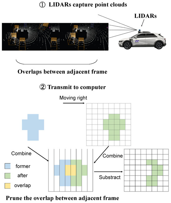
Figure 1.
Temporal correlation: significant overlaps exist in adjacent frames, and moving thing shows minor changes between frames.
Addressing this challenge requires developing techniques to effectively manage point distribution imbalance and optimize point cloud processing. One potential approach is to utilize instance-aware sampling techniques during both training and inference to ensure a more balanced representation of instances. These techniques can prioritize instances of interest or dynamically adjust the sampling strategy based on the characteristics of the point cloud.
Not only do point clouds’ overlapping regions hamper training and inference, but their inherent characteristics also present substantial challenges for efficient computation. The hurdle when dealing with 3D point clouds lies in their unordered and sparse nature, unlike the structured format of 2D images. This fundamental difference challenges conventional convolutional neural networks (CNNs) adapted for grid-like data. Previous works have identified several approaches to address this issue. The first approach involves directly processing the point cloud data. The direct processing of point clouds requires the development of specialized network architectures capable of operating on unordered point sets, such as PointNet [9] and PointCNN [10]. While the approach mentioned above enables direct feature extraction on individual points, its computational efficiency is significantly hampered by the necessity of either handling each point separately or maintaining neighborhood information.
Another technique converts the point cloud into a volumetric representation and divides the 3D space into a grid of voxels. Although this approach facilitates conventional 3D convolutional operations, it may be computationally intensive and impractical for real-time inference, particularly with large scenes [11]. The third widely recognized approach voxelizes the point cloud and subsequently applies sparse 3D convolution [12,13,14,15]. Sparse 3D convolution effectively leverages point cloud data’s inherent sparsity, significantly reducing computational costs and making large-scale point cloud processing more feasible. Several libraries, such as MinkowskiEngine [16], Spconv [17], and Torchsparse [18,19], provide efficient implementations of sparse 3D convolution. These libraries utilize dataflows similar to Gather-GEMMs-Scatter operations to handle irregular computations in point clouds. Although the sparsity of point clouds can be efficiently leveraged, the transformation involved in Gather and Scatter operations remains exceedingly time-consuming when converting between the storage of discrete data and continuous data streams suitable for modern computational processing. Both Gather and Scatter operations involve tremendous data rearrangement, so it takes considerable time to transform irregular data into a regular format suitable for matrix multiplication. This is especially true for computing devices like CPUs because the methods used for effectively performing computations on these platforms present a significant challenge. This urgency compels us to adopt suitable methods to minimize resource expenditure on such tasks, thereby enhancing processing speed. Taking Intel’s or RISC-V’s series of CPUs as an example, they provide vector instruction sets that enable developers to more effectively utilize hardware resources for achieving high-performance computations.
To address these challenges, this work first proposes a pruning technique that uses the temporal correlation between adjacent frames to alleviate redundant calculations and speed up inference. The point cloud is stored in the tuple form and captured at a rapid pace by LiDAR. That means moving things can show changes in coordinates, while unmoving things are the opposite. Inspired by this, we prune the 3D point cloud by the temporal correlation between two adjacent frames to achieve speedup in scenarios like autonomous driving. Furthermore, given that autonomous vehicles must navigate safely at high speeds while maintaining reasonable energy consumption to support adequate computational performance, deploying high-power GPUs on autonomous vehicles is not feasible. Consequently, we leverage power-efficient computing platforms like CPUs for accelerated inference. To further speed up, we analyze the runtime bottleneck caused by the conflict between discrete storage and continuous computation in the Gather-GEMMs-Scatter data flow. We optimize the Gather and Scatter operations using SIMD techniques to alleviate these time-consuming operations. We compare it with the state-of-the-art sparse inference engine TorchSparse 2.0 to show our proposed method can achieve speedup for MinkUnet and SPVCNN without a significant accuracy loss. In particular, our SIMD-based data movement can achieve more than speedup. In summary, the contributions of this paper can be delineated as follows:
- •
- We propose a pruning technique that exploits the temporal correlations between consecutive frames to alleviate redundant computations and accelerate inference.
- •
- We optimize data movement by employing Single Instruction Multiple Data (SIMD) techniques to enhance the efficiency of the time-intensive Gather and Scatter operations within the dataflow.
2. Preliminary
In this section, we will present an overview of sparse convolution and discuss the techniques used to handle the irregular arrangement of point cloud data. Additionally, we will analyze the redundancy present in point clouds and share our insights into this aspect.
2.1. Sparse Convolution
3D sparse convolution [20] is widely used for processing point cloud data in autonomous driving. In contrast to traditional convolution, sparse convolution selectively computes only the non-zero values, eliminating redundant computations and enhancing processing efficiency. The difference between traditional and sparse convolution is shown in Figure 2. This distinction highlights the efficiency of sparse convolution in maintaining a sparse representation. To better introduce sparse convolution, we denote the input feature vector as , the output feature vector as , and the weight matrix as . And is a C-dimensional feature vector for the coordinates in a D-dimensional space. represents the weight, where K is the shape of the kernel offset, D is the spatial space dimension. The weight can be divided into matrices of size , which are denoted as for . Then, the convolution can be represented as follows.
where , and it represents all non-empty neighbor voxels around center p. When s is 1, the input coordinates are the same as the output coordinates. The whole sparse convolution is shown in Figure 3, as follows: the sparse convolution will build a Hash table based on the input coordinates, and output coordinates will query the table. Upon a query hit, the corresponding inputs and weights are connected via a Gather operation, followed by matrix multiplication. The Scatter operation then aggregates the partial sums of each output value and distributes them back to their respective output positions.
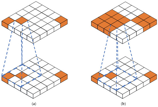
Figure 2.
Sparse convolution computes only when the center overlaps with a non-zero value when the calculation is performed. However, every non-zero value needs to multiply with every weight and will dilate very quickly in conventional convolutions. (a) Sparse convolution, (b) conventional convolution.
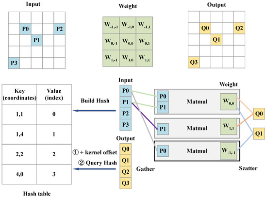
Figure 3.
Mapping and Gather-GEMMs-Scatter in sparse convolution.
2.2. Redundancy of Point Clouds
Despite the extensive adoption of sparse convolution in 3D object detection, the substantial presence of background points remains a significant challenge that requires effective resolution. As shown in Figure 1, these data are represented as discrete points due to the rapid capture speed of point cloud data by devices such as LiDAR and motion cameras [21]. Consequently, successive frames tend to have overlapping regions (temporal correlation) when objects are in motion. The information within these overlapping regions has already been extracted in the preceding frame. The redundant extraction of this information in subsequent frames results in the inefficient utilization of computational resources. Thus, it is imperative to devise strategies that mitigate redundancy to optimize computational efficiency. As shown in Figure 4, adjacent keyframes in the real world exhibit temporal correlation (i.e., significant overlap), predominantly comprising background information or less critical objects, in contrast to the more valuable foreground objects. This redundancy highlights the necessity for techniques that can effectively prioritize and isolate key foreground elements.

Figure 4.
Adjacent keyframes from CAM_FRONT in nuScenes.
2.3. Scalar Operations and SIMD Operations
Scalar operations simultaneously process a single data element, executing instructions sequentially, as shown in Figure 5. This approach can be efficient for simple tasks but often leads to significant latency when handling large datasets or complex computations. Conversely, SIMD operations enhance performance by processing multiple data elements simultaneously, with a single instruction. This parallelism greatly accelerates computation, especially in tasks with high data parallelism, by reducing the number of instruction cycles required for large-scale data processing.
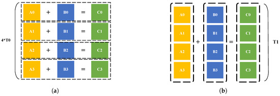
Figure 5.
(a) Scalar operation and (b) SIMD operation. The computation traditionally requires four cycles to complete; leveraging SIMD reduces this to a single cycle.
Although individual SIMD instructions, which operate on multiple data elements in parallel, may consume slightly more time than single scalar operations, the aggregate time required for SIMD to process an equivalent dataset is significantly less than that for scalar operations. This efficiency gain arises from the fact that SIMD reduces the total number of instruction cycles required, thereby accelerating the overall computation process. As a result, SIMD operations offer significant speedup and efficiency improvements over traditional scalar operations.
During Gather and Scatter operations in sparse convolution, point cloud data frequently need to transition between continuity and sparsity to accommodate the demands of matrix multiplication and the propagation between different convolutional layers. Performing these operations with scalar computation can lead to prolonged computation cycles. However, leveraging SIMD techniques to accelerate these operations can significantly reduce the computation cycles while maintaining nearly constant time per operation, thereby achieving substantial speedup.
3. Methods
In this section, we will provide a detailed explanation of how to prune points in an almost stationary continuous point cloud and how to utilize SIMD vector parallelism to accelerate the Gather-GEMMs-Scatter data flow to further speed up the process.
3.1. Prune Method for Redundancy of Point Clouds
In submanifold convolutions, the output coordinates are the same as the input coordinates when the input stride s is 1, as follows.
Employing sparse convolution techniques can effectively preserve the data’s inherent sparsity, ensuring efficient computation and resource utilization. But when the input stride s is 2, or has other values, to execute a downsampling operation or max-pooling, both background and foreground points dilate simultaneously. According to Equation , the output coordinates need to be changed. As shown in Figure 6, the input coordinates must first be offset to derive the output coordinates. Subsequently, potential output points within the expanded neighborhood of the input coordinates are identified. The final output coordinates are then selected according to the stride of the input coordinates, ensuring precise and accurate placement. These can be expressed as follows.
where % represents mod.
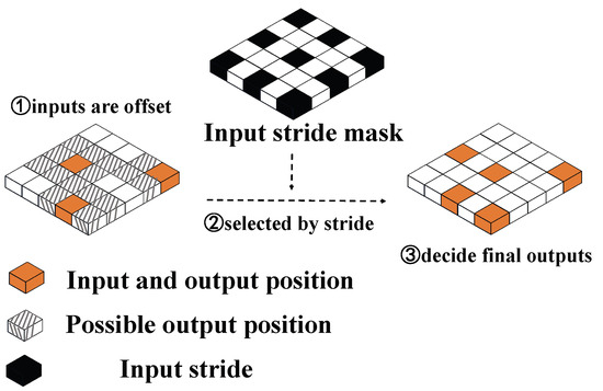
Figure 6.
Downsampling or maxpooling operation. Here, the input stride is 2.
This process could disrupt the sparsity of the input points because the background points tend to occupy a significant portion of the points, which indicates that background points will dilate more quickly than foreground points. As illustrated in Figure 3, sparse convolution relies on a hash table that establishes the relationship between input and output coordinates, thereby facilitating computations. The faster the expansion of background points, the more significant the increase in the length of the hash table, leading to a rapid growth in the computational load of the entire sparse convolution. This escalation ultimately undermines the sparsity of the point cloud data, thereby negating the advantages of sparse convolution, as shown in Figure 7.
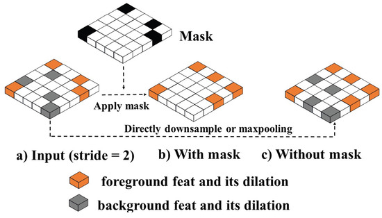
Figure 7.
Comparison of pruned and unpruned models. If foreground and background are equally treated, the sparsity will be compromised, and the computational complexity will increase significantly.
In the domain of 2D image analysis, one approach to enhancing computational speed and efficiency involves generating masks to flag features that should be ignored [22,23,24,25]. This motivates us to investigate analogous mask application techniques to 3D point clouds. Inspired by the unequal diffusion rate, we propose a pruning method based on the difference of coordinates in adjacent keyframes during the downsampling operation. The difference in coordinates is defined as follows.
where , t represents the coordinates at the t-timeslot, and m denotes the index of the point. The difference between background points tends to be small, and foreground points are the opposite. So, we define a mask based on the coordinate difference to decide which point is more likely to be the background point, as follows:
represents the sum of squared coordinate differences and is expressed as follows:
This implies that for any given point m at t-timeslot, the coordinate displacement is measured as , and a smaller displacement corresponds to a smaller .
To decide the threshold T, which is a value in the collection of all points’ coordinate displacement at t-timeslot, we should first sort the in ascending order and mark it as . Subsequently, we establish a pruning ratio() to denote the proportion of points that should be considered background points. Then, we multiply the pruning ratio with the length of (l) to find the index() of the last background point, and the last background point’s value is set as the threshold T. The index is defined as follows.
Then, we perform indexing operations on the to obtain the threshold T.
Any point falling below this threshold will result in a mask with false values at the corresponding locations, thus ensuring the precise identification and handling of sub-threshold data points.
To identify an appropriate threshold T, we conducted an investigation using a mini dataset from nuScenes. We analyzed the changes in the number of points for foreground and background categories at a pruning ratio of 0.3, 0.5, and 0.7. The results revealed that when the pruning ratio T is around 0.3, there is a significant reduction in the number of background points, while the reduction in foreground points is minimal and can be considered negligible. Therefore, it is recommended that the pruning ratio T be set around 0.3.
This mask clearly differentiates background and foreground points, facilitating accurate segmentation and analysis.
Applying a mask allows the downsampling operation to be performed only on the selected points, significantly reducing the required computations, as shown in Figure 7. According to Equations (4) and (6), this progress can be expressed as follows.
Then, the output coordinates can be represented as:
As shown in Figure 8, the pruning method is applied on the first downsample layer of the encoder because the information of coordinate differences is more precise than after the downsampling operation, which generates new coordinate information that is harder to be used again to prune points.
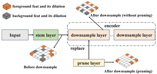
Figure 8.
Prune operation overview.
3.2. Optimization for Gather-GEMMs-Scatter
Unlike 2D images, where computations can be performed by continuously sliding a convolution window, sparse convolution relies on mapping operations. A common implementation records the coordinates of non-zero inputs in a hash table with entries of the form . After mapping, sparse convolution queries the hash table to retrieve the inputs associated with each kernel. These inputs are then rearranged to meet the continuity requirements for subsequent matrix multiplication. Once the computation is completed, the results need to be scattered back to their respective output positions. This entire process is referred to as the Gather-GEMMs-Scatter dataflow. Matrix multiplication is the core component of sparse convolution, and it takes up about 20–50% of the whole execution time [19]. However, the data orchestration process, which aims to make the data more regular, consumes a significant portion of the execution time, accounting for nearly half of it. Therefore, optimizing the Gather-Scatter operations can accelerate the overall execution time.
Considering the parallelism of the modern CPU platform, we use SIMD to execute Gather–Scatter operations in parallel. As shown in Figure 5, SIMD technology utilizes vector registers or vector processors to perform the same operation on a batch of data simultaneously. Under the control of a single instruction, the vector processor can process multiple data elements at once, significantly improving computational efficiency and performance. This means more data can be processed within the same time on CPU.
For sparse convolution, as shown in Figure 3, it is expected to perform matrix multiplication for each unique kernel weight to obtain partial sums, which are then added together to obtain the final result. During Gather and Scatter operations, the first step involves extracting the parts of the discontinuous point cloud data that are involved in the current kernel calculation and arranging them in a continuous sequence for the next operation (in the Scatter operation, the continuous data are placed back in their original position), as shown in Figure 9. In this step, data is read in batches of channel size and then switched to another position. Compared with scalar operation, the efficient utilization of SIMD operations allows for parallel acceleration along the channel dimension, enabling the simultaneous processing of multiple data points. This approach significantly enhances computational speed, optimizing performance in high-dimensional data processing tasks.
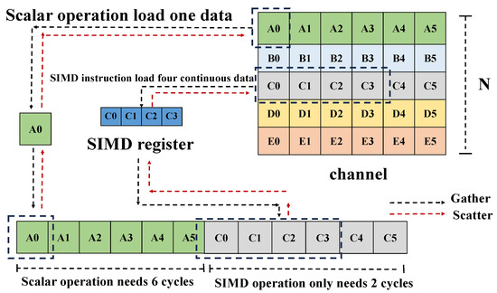
Figure 9.
Comparison of scalar and SIMD Gather–Scatter operations.
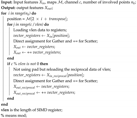
In SIMD operations, channel-wise batched data are truncated based on the length of the vector register rather than reading one data point at a time from the cache or memory. In scenarios where the channel number is not an integer multiple of the SIMD vector register length, it is imperative to fetch data of the SIMD vector register length from the tail end of the batch rather than using the pad. This precaution prevents errors stemming from array out-of-bounds access, thereby maintaining the computation’s integrity and accuracy. The detailed steps are outlined in Algorithm 1.
Complexity Analysis: The original complexity was O() due to the need for nested two-layer for loops during the Gather and Scatter operations. After implementing SIMD rewriting, the number of iterations in the inner loop is significantly reduced, especially when the number of input and output channels is small (the number of iterations in the inner for loop is determined by these two channel counts). In this case, the inner loop iterations can be considered as constant relative to the outer loop iterations, leading to a time complexity that can be viewed as O(N). However, when the number of channels is large, the size restrictions of vector registers make it challenging to substantially reduce the number of iterations in the inner loop. In this scenario, the time complexity may degrade back to O(), although it will still perform faster than the original unmodified version.
With the optimization of SIMD in the Gather and Scatter operation, the performance of the submanifold is significantly enhanced.
| Algorithm 1: SIMD optimization for Gather and Scatter. |
 |
4. Experiment
4.1. Experiment Setting
We perform all our experiments on a desktop with an Intel Xeon Gold 6230R Processor (Intel, Santa Clara, CA, USA) with an NVIDIA RTX A5000 GPU (NVIDIA, Santa Clara, CA, USA). We build TorchSparse 2.0 [18] based on Pytorch 2.0, CUDA 11.8. We evaluate the optimized Gather-GEMMs-Scatter dataflow of Torchsparse 2.0 [18] and the pruning method with the models MinkUnet42 [16] and SPVCNN [26] on datasets nuScenes-LiDARSeg [21] and SemanticKITTI [27]. To better visualize the optimization effect of Gather and Scatter, we have constructed a network that only has convolution layers with a kernel size of 3 and a stride of 1. The number of channels is increased from 4 to 256 and then reduced from 256 to 10 to simulate a simple ten-class classification network. We also compare the time consumption of the two models and their pruned versions. We set the pruning ratio as 0.3 for nuScenes-LiDARSeg (0.2 for SemanticKITTI) and replace the first encoder layer of MinkUnet [16] and SPVCNN [26] with the pruned encoder layer.
4.2. Main Results
4.2.1. Pruned
We evaluate the MinkUnet model and SPVCNN model on the 3D semantic segmentation dataset nuScenes-LiDARSeg [21] and SemanticKITTI [27]. nuScenes-LiDARSeg contains 1000 driving scenes from Boston and Singapore. The 20-second scenes are manually selected to show a diverse and interesting set of driving maneuvers, traffic situations, and unexpected behaviors. We train MinkUnet and its pruned model on the nuScenes-LiDARSeg/SemanticKITTI dataset and report the mean intersection-over-union (mIoU) on them. On the nuScenes-LiDARSeg dataset, the pruning ratio is set as 0.3 and 0.2 for the SemanticKITTI dataset because the SemanticKITTI dataset is denser than the nuScenes-LiDARSeg. All statistical results are listed in Table 1 and Table 2, expressed as ratios against the results of the best baseline. In these tables, the bolded portions represent the differences between the pruned model and the best-performing model of that category. Negative values indicate a decline in performance, while positive values signify an improvement in performance.

Table 1.
Comparison with other methods on nuScenes-LiDARSeg. All the results are normalized.

Table 2.
Comparison with other methods on SemanticKITTI. All the results are normalized.
Due to its static nature, the background class is highly likely to be pruned, resulting in a noticeable decrease in the corresponding Intersection over Union (IOU). Compared to the benchmark, the IOU loss for background classes is approximately 10%. The observed results can be attributed to the substantial overlap within the background categories. For instance, in the nuScenes-LiDARSeg dataset, the “Driveable surface" class, and in the SemanticKITTI dataset, the “Building” and “Road” classes exhibit significant overlap. This overlap leads to a noticeable decline in accuracy for these categories. However, this pruning of the background creates opportunities for enhanced feature extraction from classes that comprise a smaller proportion of the point cloud data, thereby improving their accuracy. Subtracting the background allows the model to allocate more resources to the foreground classes, which often contain essential information for various tasks. Consequently, improving the IOU for these foreground classes can effectively compensate for the reduction of IOU for the background classes. This dynamic balance ensures that the mIOU remains nearly unchanged.
This nuanced pruning strategy highlights the potential for selectively reducing background data redundancy while bolstering the accuracy of critical foreground categories. Such an approach emphasizes the importance of targeted pruning mechanisms that can judiciously differentiate between background and foreground points, thereby maintaining overall model performance while achieving greater computational efficiency. This balance is particularly crucial for applications requiring real-time processing and high precision, underscoring the need for sophisticated pruning algorithms to optimize both speed and accuracy. The decrease in background classes’ IOU can be compensated by the improvement in foreground classes, making the mIOU nearly unchanged.
As shown in Table 3, we use 23 scenes in nuScenes-LiDARSeg val split (about 900 contiguous keyframes) and 200 contiguous frames in SemanticKITTI val split to evaluate latency. On the SemanticKITTI dataset, MinkUnet (pruned) can achieve more than speedup and speedup to SPVCNN (pruned) compared to their unpruned version. On the nuScenes-LiDARSeg dataset, the speedup is slightly more significant than SemanticKITTI. MinkUnet and SPVCNN achieve and speedup on the nuScenes-LiDARSeg dataset. In general, many redundancies in point clouds can be pruned to obtain higher speeds.

Table 3.
Results of average latency (s) on SemanticKITTI and nuScenes-LiDARSeg val set.
4.2.2. Optimized Gather–Scatter
We use the easy network mentioned above to demonstrate the acceleration effect. We use the Pytorch profiler tool to evaluate the acceleration effect. The network is repeated 100× with inputs, and then, we calculate its average time consumption in Gather, Scatter, and GEMMs operations on CPU, as shown in Table 4 and Table 5. The proportion of each component is shown in Figure 10. Compared to the original Gather-GEMMs-Scatter data flow, the optimized Gather-GEMMs-Scatter data flow demonstrates a significant speedup. This is because the former operations of Gather and Scatter use OMP multithreading, where the overhead of creating new threads is much more significant than the computation time on each thread. This means that the required data need to be moved from memory to the corresponding thread each time, resulting in the majority of time spent on this part. The speedup ratio decreases as the network depth increases, caused by the supported number of bits in the SIMD instruction set. For example, the 256-bit SIMD instruction can simultaneously process eight 32-bit single-precision floating-point datasets.

Table 4.
Different layers’ time consumption and its speedup (channels ranging from 4 to 256).

Table 5.
Different layers’ time consumption and speedup (channels ranging from 256 to 10 with transposed).
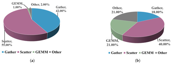
Figure 10.
Proportion of each component. (a) Original version; (b) SIMD version.
However, as the number of channels increases, the number of operations to be processed increases, decreasing the speedup. As shown in Table 4 and Table 5, when the number of channels is doubled, the decrease in the speedup ratio is also proportional. The decrease in the speedup ratio is slightly smaller in channel (4, 8) than in channel (8, 16). This is because channels (4, 8) use a 128-bit SIMD instruction, while channels (8, 16) use a 256-bit SIMD instruction, which is faster than the 128-bit SIMD instruction.
Also, we compared SIMD’s time consumption with that of its pruned version in Table 6. With optimized Gather and Scatter operations, each inference time consumption on the pruned and unpruned models is vastly decreased. On the nuScenes-LiDARSeg dataset, MinkeUnet (SIMD) and MinkUnet (prune+SIMD) achieve speedup and speedup compared to MinkUnet and MinkUnet (prune). SPVCNN (SIMD) and SPVCNN (prune+SIMD) achieve speedup and speedup compared to SPVCNN and SPVCNN (prune). On the SemanticKITTI dataset, MinkeUnet (SIMD) and MinkUnet (prune+SIMD) achieve speedup and speedup compared to MinkUnet and MinkUnet (prune), and SPVCNN (SIMD) and SPVCNN (prune+SIMD) achieve speedup and speedup compared to SPVCNN and SPVCNN (prune).

Table 6.
Results of average latency (s) on SemanticKITTI and nuScenes-LiDARSeg val set. MinkUnet (SIMD) and SPVCNN (SIMD) denote the optimized Gather-GEMMs-Scatter dataflow.
4.2.3. Ablation Study on the Pruning Ratio
We also investigated the impact of pruning magnitude on model performance and acceleration ratio, as depicted in Figure 11 and Figure 12. mIOU is normalized as the ratio to the unpruned version. Our analysis indicates that with an increment in pruning intensity, a discernible degradation in the mean Intersection over Union (mIOU) is observed. This decrement is primarily attributable to the shift in the categorical composition of the pruned points, which transitions progressively from background to foreground categories with increasing levels of pruning. In particular, substantial overlap exists in the background category within adjacent frames of point clouds. Consequently, most of the pruning points are categorized under the background when the pruning intensity ranges between 0.3 and 0.4 on nuScenes-LiDARSeg and 0.2 and 0.3 on SemanticKITTI. However, it is noteworthy that the foreground categories also exhibit a degree of overlap. As the pruning intensity further escalates, points associated with the foreground category are also excised, precipitating a pronounced decline in accuracy.
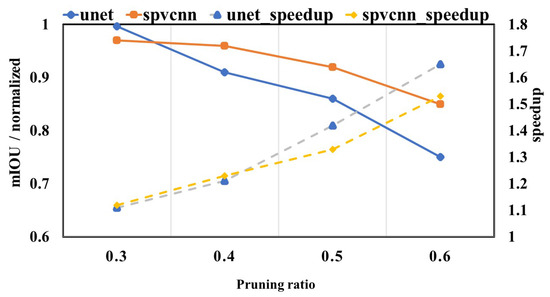
Figure 11.
Different pruning ratios on nuScenes-LiDARSeg. The mIOU is normalized.
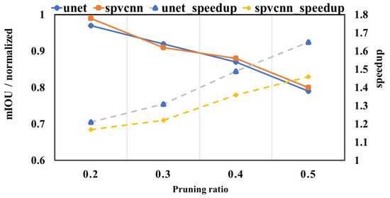
Figure 12.
Different pruning ratios on SemanticKITTI. The mIOU is normalized.
This phenomenon underscores the delicate balance required in pruning strategies, which aims to maximize computational efficiency while minimizing the adverse impact on model performance. Effective pruning algorithms must, therefore, account for the intricate composition of point cloud data, ensuring that foreground information critical to task performance is preserved as much as possible. This careful consideration is essential for achieving optimal trade-offs between acceleration and accuracy, thereby enhancing the practical applicability of pruning techniques in real-world scenarios.
5. Conclusions
Inspired by the redundancy in 3D point cloud data, this paper proposes a pruning method based on the coordinate differences in adjacent frames. We evaluate this method using MinkUNet and SPVCNN on the nuScenes-LiDARSeg and SemanticKITTI datasets, achieving a speedup. This approach highlights the efficacy of optimizing data handling and leveraging spatiotemporal redundancies to enhance performance. Also, we employ Single Instruction Multiple Data (SIMD) to optimize sparse convolution using a Gather-GEMMs-Scatter dataflow, achieving an average speedup of more than on the two models. By intelligently reducing the computational load through SIMD optimization and targeted pruning, we demonstrate significant improvements in processing speed and model efficiency. These proposed techniques underscore the potential for advanced optimization techniques to make real-time 3D point cloud processing more feasible and effective in practical applications. Future work will build upon this study to further investigate the optimization of sparse convolution operators and develop new acceleration algorithms, aiming to meet the increasing demand for the efficient processing of point cloud data.
Author Contributions
Resources, C.Z., Q.Y., W.L. and Z.X.; Data curation, L.C.; Writing—original draft, L.C.; Writing—review & editing, L.C. and Z.X. All authors have read and agreed to the published version of the manuscript.
Funding
This research was funded by the National Natural Science Foundation of China under Grant 62105163, the Fundamental Research Funds for the Central Universities under Grant NJ2023020, and the Natural Science Research Foundation of Jiangsu Province for Youth under Grant BK20220398.
Institutional Review Board Statement
Not applicable.
Informed Consent Statement
Not applicable.
Data Availability Statement
The original contributions presented in this study are included in the article. Further inquiries can be directed to the corresponding author.
Conflicts of Interest
Author Qunsong Ye was employed by the company Shenzhen Index Technology Co., Ltd. The remaining authors declare that the research was conducted in the absence of any commercial or financial relationships that could be construed as a potential conflict of interest.
References
- Zhu, Q.; Fan, L.; Weng, N. Advancements in point cloud data augmentation for deep learning: A survey. Pattern Recognit. 2024, 153, 110532. [Google Scholar]
- Krawczyk, D.; Sitnik, R. Segmentation of 3D point cloud data representing full human body geometry: A review. Pattern Recognit. 2023, 139, 109444. [Google Scholar] [CrossRef]
- Xu, Y.; Tuttas, S.; Hoegner, L.; Stilla, U. Voxel-based segmentation of 3D point clouds from construction sites using a probabilistic connectivity model. Pattern Recognit. Lett. 2018, 102, 67–74. [Google Scholar] [CrossRef]
- Bhattacharyya, P.; Czarnecki, K. Deformable PV-RCNN: Improving 3D object detection with learned deformations. arXiv 2020, arXiv:2008.08766. [Google Scholar]
- Xu, S.; Zhou, D.; Fang, J.; Yin, J.; Bin, Z.; Zhang, L. Fusionpainting: Multimodal fusion with adaptive attention for 3D object detection. In Proceedings of the 2021 IEEE International Intelligent Transportation Systems Conference (ITSC), Indianapolis, IN, USA, 19–22 September 2021; pp. 3047–3054. [Google Scholar]
- Yin, T.; Zhou, X.; Krähenbühl, P. Multimodal virtual point 3D detection. Adv. Neural Inf. Process. Syst. 2021, 34, 16494–16507. [Google Scholar]
- Liu, J.; Chen, Y.; Ye, X.; Tian, Z.; Tan, X.; Qi, X. Spatial pruned sparse convolution for efficient 3D object detection. Adv. Neural Inf. Process. Syst. 2022, 35, 6735–6748. [Google Scholar]
- Chen, Y.; Li, Y.; Zhang, X.; Sun, J.; Jia, J. Focal sparse convolutional networks for 3D object detection. In Proceedings of the IEEE/CVF Conference on Computer Vision and Pattern Recognition, New Orleans, LA, USA, 18–24 June 2022; pp. 5428–5437. [Google Scholar]
- Qi, C.R.; Su, H.; Mo, K.; Guibas, L.J. Pointnet: Deep learning on point sets for 3D classification and segmentation. In Proceedings of the IEEE Conference on Computer Vision and Pattern Recognition, Honolulu, HI, USA, 21–26 July 2017; pp. 652–660. [Google Scholar]
- Li, Y.; Bu, R.; Sun, M.; Wu, W.; Di, X.; Chen, B. Pointcnn: Convolution on x-transformed points. Adv. Neural Inf. Process. Syst. 2018, 31. [Google Scholar]
- Qi, C.R.; Su, H.; Nießner, M.; Dai, A.; Yan, M.; Guibas, L.J. Volumetric and multi-view cnns for object classification on 3D data. In Proceedings of the IEEE Conference on Computer Vision and Pattern Recognition, Las Vegas, NV, USA, 27–30 June 2016; pp. 5648–5656. [Google Scholar]
- Zhou, Y.; Tuzel, O. Voxelnet: End-to-end learning for point cloud based 3D object detection. In Proceedings of the IEEE Conference on Computer Vision and Pattern Recognition, Salt Lake City, UT, USA, 18–22 June 2018; pp. 4490–4499. [Google Scholar]
- Shi, S.; Guo, C.; Jiang, L.; Wang, Z.; Shi, J.; Wang, X.; Li, H. Pv-rcnn: Point-voxel feature set abstraction for 3D object detection. In Proceedings of the IEEE/CVF Conference on Computer Vision and Pattern Recognition, Seattle, WA, USA, 14–19 June 2020; pp. 10529–10538. [Google Scholar]
- Deng, J.; Shi, S.; Li, P.; Zhou, W.; Zhang, Y.; Li, H. Voxel r-cnn: Towards high performance voxel-based 3D object detection. In Proceedings of the AAAI Conference on Artificial Intelligence, Online, 2–9 February 2021; Volume 35, pp. 1201–1209. [Google Scholar]
- Yin, T.; Zhou, X.; Krahenbuhl, P. Center-based 3D object detection and tracking. In Proceedings of the IEEE/CVF Conference on Computer Vision and Pattern Recognition, Nashville, TN, USA, 20–25 June 2021; pp. 11784–11793. [Google Scholar]
- Choy, C.; Gwak, J.; Savarese, S. 4d spatio-temporal convnets: Minkowski convolutional neural networks. In Proceedings of the IEEE/CVF Conference on Computer Vision and Pattern Recognition, Long Beach, CA, USA, 16–17 June 2019; pp. 3075–3084. [Google Scholar]
- Contributors, S. Spconv: Spatially Sparse Convolution Library. 2022. Available online: https://github.com/traveller59/spconv (accessed on 15 March 2025).
- Tang, H.; Yang, S.; Liu, Z.; Hong, K.; Yu, Z.; Li, X.; Dai, G.; Wang, Y.; Han, S. Torchsparse++: Efficient training and inference framework for sparse convolution on gpus. In Proceedings of the IEEE/ACM International Symposium on Microarchitecture (MICRO), Toronto, ON, Canada, 28 October–1 November 2023; pp. 225–239. [Google Scholar]
- Tang, H.; Liu, Z.; Li, X.; Lin, Y.; Han, S. Torchsparse: Efficient point cloud inference engine. Proc. Mach. Learn. Syst. 2022, 4, 302–315. [Google Scholar]
- Graham, B.; Engelcke, M.; Van Der Maaten, L. 3D semantic segmentation with submanifold sparse convolutional networks. In Proceedings of the IEEE Conference on Computer Vision and Pattern Recognition, Salt Lake City, UT, USA, 18–22 June 2018; pp. 9224–9232. [Google Scholar]
- Caesar, H.; Bankiti, V.; Lang, A.H.; Vora, S.; Liong, V.E.; Xu, Q.; Krishnan, A.; Pan, Y.; Baldan, G.; Beijbom, O. nuscenes: A multimodal dataset for autonomous driving. In Proceedings of the IEEE/CVF Conference on Computer Vision and Pattern Recognition, Seattle, WA, USA, 13–19 June 2020; pp. 11621–11631. [Google Scholar]
- Dong, X.; Huang, J.; Yang, Y.; Yan, S. More is less: A more complicated network with less inference complexity. In Proceedings of the IEEE Conference on Computer Vision and Pattern Recognition, Honolulu, HI, USA, 21–26 July 2017; pp. 5840–5848. [Google Scholar]
- Ren, M.; Pokrovsky, A.; Yang, B.; Urtasun, R. Sbnet: Sparse blocks network for fast inference. In Proceedings of the IEEE Conference on Computer Vision and Pattern Recognition, Salt Lake City, UT, USA, 18–22 June 2018; pp. 8711–8720. [Google Scholar]
- Verelst, T.; Tuytelaars, T. Dynamic convolutions: Exploiting spatial sparsity for faster inference. In Proceedings of the IEEE/CVF Conference on Computer Vision and Pattern Recognition, Seattle, WA, USA, 13–19 June 2020; pp. 2320–2329. [Google Scholar]
- Xie, Z.; Zhang, Z.; Zhu, X.; Huang, G.; Lin, S. Spatially adaptive inference with stochastic feature sampling and interpolation. In Proceedings of the Computer Vision–ECCV 2020: 16th European Conference, Glasgow, UK, 23–28 August 2020; Proceedings, Part I 16. Springer: Berlin/Heidelberg, Germany, 2020; pp. 531–548. [Google Scholar]
- Tang, H.; Liu, Z.; Zhao, S.; Lin, Y.; Lin, J.; Wang, H.; Han, S. Searching efficient 3D architectures with sparse point-voxel convolution. In Proceedings of the European Conference on Computer Vision, Glasgow, UK, 23–28 August 2020; Springer: Berlin/Heidelberg, Germany, 2020; pp. 685–702. [Google Scholar]
- Behley, J.; Garbade, M.; Milioto, A.; Quenzel, J.; Behnke, S.; Stachniss, C.; Gall, J. Semantickitti: A dataset for semantic scene understanding of lidar sequences. In Proceedings of the IEEE/CVF international Conference on Computer Vision, Seoul, Repiblic of Korea, 27 October–2 November 2019; pp. 9297–9307. [Google Scholar]
- Li, S.; Chen, X.; Liu, Y.; Dai, D.; Stachniss, C.; Gall, J. Multi-scale interaction for real-time lidar data segmentation on an embedded platform. IEEE Robot. Autom. Lett. 2021, 7, 738–745. [Google Scholar]
- Zhang, Y.; Zhou, Z.; David, P.; Yue, X.; Xi, Z.; Gong, B.; Foroosh, H. Polarnet: An improved grid representation for online lidar point clouds semantic segmentation. In Proceedings of the IEEE/CVF Conference on Computer Vision and Pattern Recognition, Seattle, WA, USA, 13–19 June 2020; pp. 9601–9610. [Google Scholar]
- Xu, C.; Wu, B.; Wang, Z.; Zhan, W.; Vajda, P.; Keutzer, K.; Tomizuka, M. Squeezesegv3: Spatially-adaptive convolution for efficient point-cloud segmentation. In Proceedings of the Computer Vision–ECCV 2020: 16th European Conference, Glasgow, UK, 23–28 August 2020; Proceedings, Part XXVIII 16. Springer: Berlin/Heidelberg, Germany, 2020; pp. 1–19. [Google Scholar]
Disclaimer/Publisher’s Note: The statements, opinions and data contained in all publications are solely those of the individual author(s) and contributor(s) and not of MDPI and/or the editor(s). MDPI and/or the editor(s) disclaim responsibility for any injury to people or property resulting from any ideas, methods, instructions or products referred to in the content. |
© 2025 by the authors. Licensee MDPI, Basel, Switzerland. This article is an open access article distributed under the terms and conditions of the Creative Commons Attribution (CC BY) license (https://creativecommons.org/licenses/by/4.0/).