Comparison and Interpretability Analysis of Deep Learning Models for Classifying the Manufacturing Process of Pigments Used in Cultural Heritage Conservation

Abstract

This study investigates the classification of pigment-manufacturing processes using deep learning to identify the optimal model for cultural property preservation science. Four convolutional neural networks (CNNs) (i.e., AlexNet, GoogLeNet, ResNet, and VGG) and one vision transformer (ViT) were compared on micrograph datasets of various pigments. Classification performance indicators, receiver-operating characteristic curves, precision–recall curves, and interpretability served as the primary evaluation measures. The CNNs achieved accuracies of 97–99%, while the ViT reached 100%, emerging as the best-performing model. These findings indicate that the ViT has potential for recognizing complex patterns and correctly processing data. However, interpretability using guided backpropagation approaches revealed limitations in the ViT ability to generate class activation maps, making it challenging to understand its internal behavior through this technique. Conversely, CNNs provided more detailed interpretations, offering valuable insights into the learned feature maps and hierarchical data processing. Despite its interpretability challenges, the ViT outperformed the CNNs across all evaluation metrics. This study underscores the potential of deep learning in classifying pigment manufacturing processes and contributes to cultural property conservation science by strengthening its scientific foundation for the conservation and restoration of historical artifacts.

1. Introduction

1.1. Overview

Pigments, essential materials in the conservation of cultural heritage and painting, are produced through both industrial synthesis and natural extraction from minerals. Distinguishing between these two production methods is challenging through visual and chemical composition analyses alone. Studies estimating the manufacturing process of pigments with identical chemical formulas and structures typically focus on classifying the crystalline form of the particles. Identifying the crystal form or microstructure of particles is typically performed using data derived from microscopes and polarized light microscopic image data atlases. However, there is a limited accumulation of microscopic image data, such as atlases. Furthermore, analyzing these micro-structured images requires experts to manually review hundreds of individual images from a single sample, confirming common particle shapes [1]. This process is time-consuming and heavily relies on the expertise of the observer.

Discrimination models have been developed using convolutional neural networks (CNNs), such as AlexNet, GoogLeNet, ResNet, and VGG, to classify pigment-manufacturing processes with over 96% accuracy [2,3]. CNNs, which are highly effective for object recognition, allow for objective and quantitative analysis of large-scale image data. Recent studies have applied CNNs across various fields [4]. In cultural heritage, CNNs are primarily used for image classification of architectural heritage and archeological topography [5,6,7]. Additionally, CNNs (e.g., VGG16, InceptionNet V3, ResNet50, and EfficientNet B0) have been used to evaluate damage in digital single-lens reflex images of wooden architectural heritage artifacts, visualizing the location of damage through a class activation map (CAM) [8]. In cultural heritage and image classification, large-scale spectrum libraries are used to fine-tune CNNs and identify material components [9,10,11]. Accurate identification of constituent elements through CNN classification techniques is crucial for the conservation of cultural heritage. When conserving and repairing cultural heritage, the principles of the Venice Charter are followed, and traditional materials are prioritized [12]. Cultural heritage sites involving pigments, such as paintings and murals, typically rely on natural mineral pigments. However, the advancement of industrial pigments since the 19th century has hindered the visual identification of pigments produced by these two methods. For example, distinguishing between red pigments like vermilion and cinnabar requires observing the fine shape of pigment particles and matching their chemical composition (i.e., Hg and S) [1,13]. A previous study successfully categorized pigment-manufacturing processes with over 96% accuracy using CNNs [2].

While CNNs have shown high classification accuracy in cultural heritage applications, their lack of interpretability and failure to suitably capture complex patterns hinder their broader applicability. Recent advancements in vision transformers (ViTs), which can efficiently process such complex data, provide an opportunity to bridge these gaps and enhance both performance and interoperability. Given its recent development, however, the application of ViTs to cultural heritage preservation remains largely unexplored.

We aim to investigate the effectiveness of ViTs for pigment-manufacturing classification, comparing them to established CNNs and addressing key challenges in both accuracy and interpretability. By training interpretable filters to identify patterns in the input images that influence predictions, we advance the classification of pigment production processes, building upon previous studies, and propose an interpretable deep learning method.

1.2. Related Work

Deep learning has proven superior for automatically extracting features from complex visual data, making it an essential technology for cultural heritage work, including artifact recognition, heritage restoration, and multimedia cultural data classification [14,15,16,17]. Early applications of deep learning in cultural heritage focused primarily on identifying archeological sites [18,19,20]. These studies classified traces of tombs, legacy marks, and topographic visualizations using aerial photographs [14,15,21]. Additionally, various studies have presented and classified architectural styles using platforms such as Blocklet [5]. Other systematic reviews have applied deep learning models like VGG, InceptionNet, ResNet, and R-CNN to classify surface damage during regular inspections of architectural cultural heritage sites [7,8]. Beyond architectural and archeological sites, some studies have applied deep learning to cultural heritage objects that are not entire buildings, archeological sites, or cities [22]. Various spectra have been used for the analysis of cultural heritage materials, and deep learning has been applied to X-ray fluorescence spectroscopy measurements [9] and near-infrared spectral data to classify samples and predict their components or changes in composition [23]. Recently, deep learning has been adopted as a strategy for the digital preservation of intangible and tangible cultural heritage, such as relics and historic sites. This approach has revolutionized how researchers and conservators engage with cultural heritage research [24,25,26,27]. For intangible cultural heritage, deep learning has enabled the documentation of performing arts and dance through the generation of vast amounts of RGB-D and 3D skeleton data. This has led to significant progress in choreography summaries and dance pose recognition using visual sensors, motion capture devices, and machine learning model [28,29]. As digital cultural heritage research continues to expand, it is expected to cover a wide range of topics and impact multiple areas of preservation and documentation. Various aspects of visual computing related to tangible and intangible cultural heritage preservation and documentation have been explored, and the field is expected to expand into more areas.

2. Materials and Methods

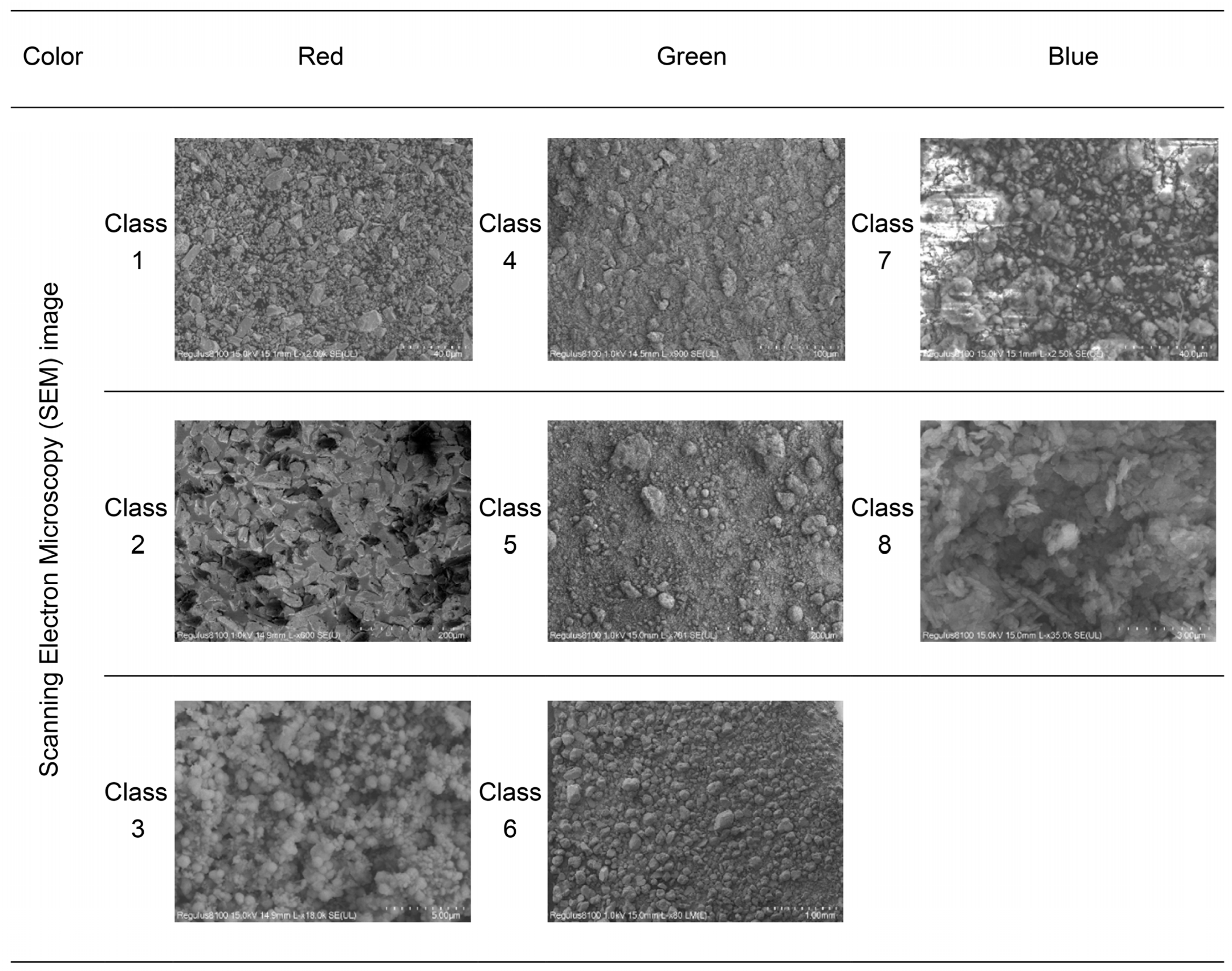
2.1. Materials

Red, green, and blue pigments are produced by natural (traditional) or industrial methods. The pigments are divided into eight classes based on their production methods and composition. Classes 1 and 2 consist of red pigments with the same chemical formula, produced using traditional methods, while class 3 consists of red pigments produced through industrial methods. Classes 4 and 5 include pigments composed of 100% copper and a mixture of 78% copper and 22% tin, respectively. Class 6 consists of green pigments produced through industrial methods. Class 7 includes indigo manufactured through traditional methods, while class 8 consists of indigo produced using industrial methods. A detailed list of the pigment classes is provided in

Table 1. Details of red, green, and blue pigments considered in this study.

Class	Color (Source)	Manufacturer	Common Name (Chemical Structure)
1	Red (traditional)	Suzhou Jiang Sixu Tang Chinese Painting Pigment Co., Ltd. (Suzhou, China)	Cinnabar (HgS)
2	Red (traditional)	GAIRART (Goyang-si, Republic of Korea)	Cinnabar (HgS)
3	Red (industrial)	GAIRART (made in Japan)	Vermillion (HgS)
4	Green (traditional)	National Research Institute of Cultural Heritage (Daejeon, Republic of Korea)	Atacamite (Cu2Cl(OH)3)
5	Green (traditional)		Atacamite (Cu2Cl(OH)3)
6	Green (industrial)	Kremer (Bad Soden-Salmünster, Germany)	Verdigris (Cu(CH3COO)2
7	Blue (traditional)	Korean traditional indigo (Republic of Korea)	Indigo + Calcite (C16H10N2O2 + CaCO3)
8	Blue (industrial)	ChemFaces (Wuhan, China)	Indigo (C16H10N2O2)

.

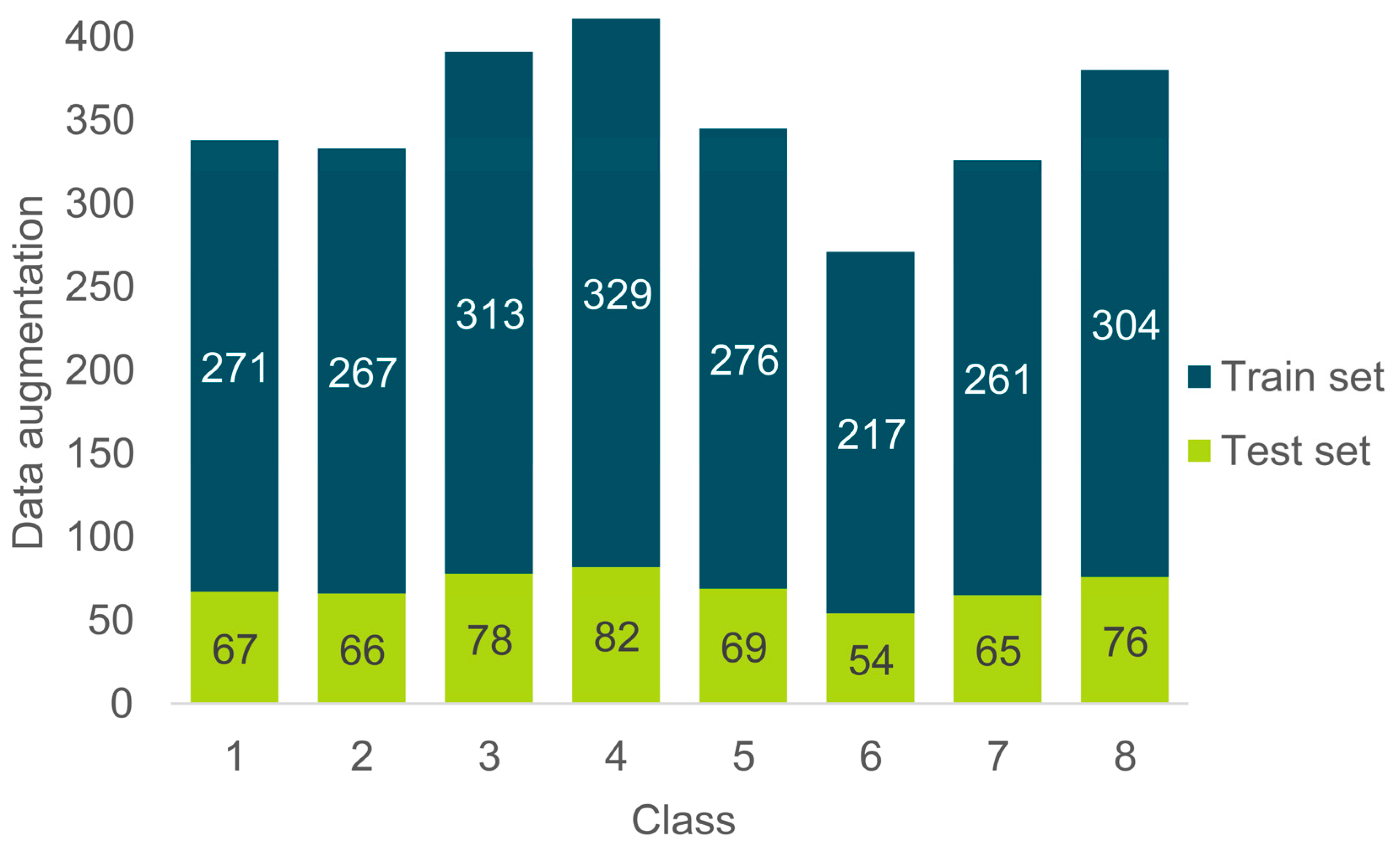
2.2. Dataset and Preprocessing

Micrograph images for the dataset were collected through scanning electron microscopy (SEM). The images were observed under a field-emission gun SEM system (Hitachi, Regulus 8100, Hong Kong) with a maximum acceleration voltage of 15 kV. The surface of the pigments was coated with platinum [13]. Each class contained approximately the same number of images to ensure a balanced dataset. Figure 1 shows examples of micrographs for each class in the collected dataset.

For the dataset, the training and test sets were split in an 8:2 ratio (Figure 2). The dataset used for the multiclass classification task comprised 2795 micrograph images distributed across eight class labels.

Geometric transformation functions were applied through data augmentation to enhance learning. Using the torchvision transform, tasks such as image rotation and flipping were performed to expand the dataset and improve the model ability to learn features.

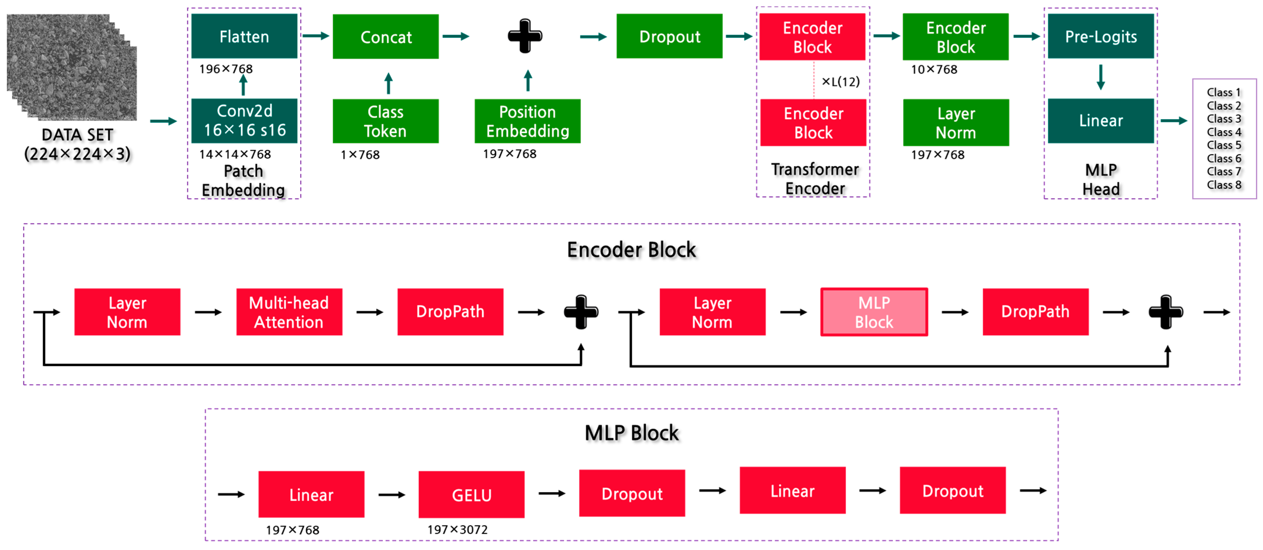
2.2.1. Proposed Approaches

Five deep learning architectures were evaluated: AlexNet, GoogLeNet, VGG16, ResNet50, and ViT. For transfer learning, pretrained weights from ImageNet, which is a 100-category object classification dataset, were used during training. As CNN models have been extensively used in previous studies, this study focuses primarily on describing the ViT.

The AlexNet architecture consists of eight layers, including five convolutional layers and three fully connected layers [30]. The network primarily comprises convolutional activation function layers, pooling layers, local response normalization, and fully connected layers.

GoogLeNet is a deep neural network model based on the inception module to address challenges such as overfitting, computational complexity, and gradient vanishing that arise as the network depth and width increase. The inception module enhances the receptive field by combining various convolutional kernels and overlapping outputs, thereby improving robustness. Multiple versions of GoogLeNet have been developed (e.g., V1–V4) [31]. For this study, the V1 version was selected to facilitate comparison with other models.

ResNets are renowned for their ability to improve accuracy with deeper layers, making them a powerful choice for computer vision tasks and recognition applications. The ResNet architecture employs residual learning to address the degradation problem associated with deep networks. Among the available versions, ResNet50 was utilized in this study for its balance between depth and computational efficiency [32].

The VGG model, developed by a group at Oxford University, is a renowned algorithm for large-scale image recognition [33]. Its performance improves as the network depth increases. The network uses only 3 × 3 convolutional kernels (with a maximum pooling size of 2 × 2). In this study, the VGG16 model was employed, comprising 13 convolutional layers, five pooling layers, three fully connected layers, and a softmax activation function for classification.

The ViT has been evaluated as an effective classification model by directly processing image patch sequences through a transformer architecture. Its relatively simple structure and excellent performance and scalability render it highly suitable for computer vision applications (Figure 3).

2.2.2. Transfer Learning and Parameter Setting

Transfer learning can be categorized into three main types: instance-based, feature-based, and parameter-based transfer learning. Because the classification of the dataset in this study primarily relies on feature factors such as edge and brightness, feature-based transfer learning was used to enhance model training. The feature extractors were migrated from the source domain to the target domain, and then these feature extractors were used to extract features of the target domain.

The feature extractor is transferred from the source domain to the target domain, where it then extracts features specific to the target domain. These extracted features pass through a multilayer model consisting of layers such as average-pooling2D, flatten, dense, and dropout. During model training, pre-trained weights from object classification tasks on the ImageNet dataset are used to fine-tune the parameters of all layers and enhance the model performance and learning (

Table 2. Hyperparameters and settings for training models.

Parameter	Value
RandomResizedCrop	224
Normalization	[0.485, 0.456, 0.406]
	[0.229, 0.224, 0.225]
Batch size	16
Number of workers	8
Optimizer	Adam
Criterion	Cross-entropy loss
Epochs	30
Step size	5
Gamma	0.5

).

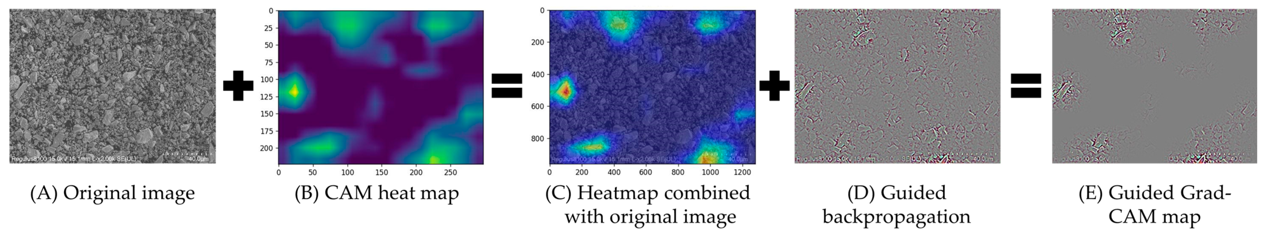
2.2.3. Visualization Method

Deep learning models consist of multiple hidden layers, making it difficult to analyze how the trained model makes decisions and derives predictions. We use a technique to increase transparency by generating visual explanations for decision-making in large-scale CNN-based modes; to enhance the interpretability of the classification results, this study employs two deep explainers: CAM and guided backpropagation. First, the heatmap (B) drawn by the first attempted CAM tends to have only a focus area and is difficult to observe intuitively. Therefore, the CAM heatmap (B) is integrated with the original image (A) and shown as (C) in Figure 4. The focus area of such a heatmap appears too small, is not clear, and has low sensitivity. To solve this problem, guided backpropagation is introduced. Guided backpropagation is a classic method of model visualization that can respond to high network positions at the pixel level by propagating the gradient backwards through the feature map and localizing the relevant regions within the micrograph by sharpening the focus area of the heatmap as in (D). Finally, for the feature map, the gradients of the target class are computed and combined to form a weighted map, emphasizing the important areas in the image (E) [34].

2.2.4. Evaluation Measures

The performance of the CNN models was evaluated using several metrics: accuracy, precision, recall, F1-score, and confusion matrix [35]. Accuracy measures the proportion of correctly classified predictions to the total number of predictions considering both positive and negative samples [6,36]:

$$Accuracy={\displaystyle \frac{TP+TN}{TP+TN+FP+FN}},$$

(1)

where TP indicates the number of true positives, TN indicates the number of true negatives, FP indicates the number of false positives, and FN indicates the number of false negatives.

Precision is the proportion of true positive predictions out of all samples predicted as positive:

$$Precision={\displaystyle \frac{TP}{TP+FP}}$$

(2)

The true positivity rate, or the percentage of all actual positives correctly classified as positive, is commonly referred to as precision. When combined with accuracy, if considered as a binary classification problem, precision reflects the accuracy for each individual category.

Recall measures the proportion of true positive predictions out of all actual positive samples:

$$Recall={\displaystyle \frac{TP}{P}},$$

(3)

where P is the total number of actual positive samples.

The F1-score is a weighted harmonic average of precision and recall based on parameter α:

$$F={\displaystyle \frac{\left({\alpha }^2+1\right) \times Precision \times Recall }{{\alpha }^2 \times Precision \times Recall}}$$

(4)

The receiver-operating characteristic (ROC) curves are visual tools used to assess the performance of a classifier across different decision thresholds. The horizontal axis represents the false positive rate (or 1-specificity), while the vertical axis shows the true positive rate (or sensitivity). Additionally, the precision–recall (PR) curve is an evaluation tool that calculates precision and recall at different thresholds and plots them, providing insights into the classifier ability to distinguish classes.

3. Results and Discussion

3.1. Evaluation of Deep Learning Models

The performance of the five models across four evaluation metrics (accuracy, precision, recall, and F1-score) for the multiclass classification task is summarized in

Table 3. Performance of the five models across four evaluation metrics.

Model	AlexNet	GoogLeNet	VGG16	ResNet50	ViT
Accuracy	0.969	0.973	0.993	0.984	1
Precision	0.970	0.973	0.993	0.984	1
Recall	0.969	0.973	0.993	0.984	1
F1-score	0.970	0.973	0.993	0.984	1

.

The accuracy of the training and test sets for all models steadily increased throughout training. As the number of epochs increased, the training accuracy improved consistently, and the test set accuracy stabilized after reaching a certain value, indicating that none of the five models experienced overfitting. VGG16 exhibited good performance with minimal variation compared to the other models. Although AlexNet showed the lowest accuracy, it still achieved a score close to 1.0 on the test set after 30 training epochs (Figure 5).

3.2. ROC and PR Curves

The ROC curves of the five models showed that most classes performed well, with nearly all class curves approaching the optimal (0.1) point. However, AlexNet, GoogleNet, and ResNet exhibited poor classification performances for class 5. Nevertheless, performance differences across most categories were not significant.

In the PR curves, AlexNet, GoogLeNet, and ResNet struggled with classes 4 and 5. This was likely because of the visual similarity of the micrographs from these classes. In contrast, ViT and VGG demonstrated robust performance, remaining unaffected by these similarities and achieving the best results (Figure 6).

3.3. Interpretability Analysis

To analyze model interpretability, CAMs were obtained as heatmaps for samples from each category based on a selected feature layer of the deep models. While each model responded differently to the sample features, they successfully classified images. Figure 7 shows the micrograph and CAM heatmap for class 2, highlighting that the VGG focus for class 2 differs significantly from those of other classes. Early in training, the CAM concentrated on broad features of the micrograph at a shallow level, including non-relevant elements such as explanatory text and scale information at the bottom of the image as Figure 7B,C. As training progressed, the focus shifted away from these areas, gradually highlighting the most relevant regions, such as the particle shapes within the micrograph (Figure 7D,E). This shift culminated in final CAM result emphasizing important areas (Figure 7F). These findings suggest that the deep learning models effectively captured and classified particle shape differences, aligning with the study objective of particle shape classification.

Even within the same deep learning model, each particle shape feature of the sample responds differently, contributing to effective image classification. However, when comparing the VGG model and ViT for class 1 in Figure 8, differences in defocusing are evident in the guided backpropagation and guided backpropagation-CAM images. This defocusing effect reduces CAM precision in the ViT, as the input image is divided into multiple patches during processing. When these patches are reassembled into the heatmap, the result is blurry. Unlike the four CNNs, which compute Grad-CAM by weighting feature maps across channels, ViT weighs feature maps across patches, which maintain uniform feature map alignment with the original image size. Nevertheless, Grad-CAM remains effective in interpreting and visualizing decision-making processes and outcomes in micrograph images. The ViT model demonstrated the highest classification accuracy; however, the class activation mapping (CAM) heatmap was less focused. While this suggests that the ViT model is well-suited for classification tasks, it may not be the most optimal choice for studies requiring high interpretability.

4. Conclusions

This study applied deep learning approaches to evaluate CNNs and ViT in their effectiveness for distinguishing the manufacturing processes of natural and industrial pigments and supporting interpretable decision-making within deep learning models. Based on the evaluation metrics, ViT demonstrated the best performance among all models. The classification results for the ViT test set were entirely accurate, confirming ViT as the state-of-the-art algorithm on this dataset. It successfully addressed the limitations of existing CNNs. To enhance interpretability, CAM was used to utilized to visualize the decision-making process of the deep learning models and improve the understanding of their relationship with the dataset. Guided backpropagation-CAM provided detailed heatmaps for all CNNs, recognizing the pigment shapes within the micrographs, displaying heatmaps at the pixel level, and facilitating observation and analysis by experts. However, while ViT achieved perfect classification based on performance metrics, its interpretability remains a significant challenge because of the inherent limitations in its architecture. The defocusing phenomenon observed in ViT results reduces its capacity for detailed decision interpretation. Future research should focus on developing methods that enhance detailed decision interpretation while maintaining or surpassing the performance of existing models.

5. Patent

The methodology described in this study is part of a patent application currently under review in Korea (Method and Apparatus for Classifying Micro-Morphological Image Based on Deep Learning to Determine Manufacturing Process of Mineral Pigment, University Science and Technology Beijing).

References

1. Eastaugh, N.; Walsh, V.; Siddall, R. Pigment Compendium-Dictionary and Optical Microscopy of Historical Pigments; Routledge: London, UK, 2018. [Google Scholar]
2. Go, I.; Ma, X.; Guo, H. CNN-based deep learning method for classifying micro-form images of pigments with different manufacturing processes. Herit. Sci. 2025, preprint. [Google Scholar]
3. Zhong, X.; Gallagher, B.; Eves, K.; Robertson, E.; Mundhenk, T.N.; Han, T.Y.-J. A study of real-world micrograph data quality and machine learning model robustness. Npj Comput. Mater. 2021, 7, 161. [Google Scholar] [CrossRef]
4. Leksut, J.T.; Zhao, J.; Itti, L. Learning visual variation for object recognition. Image Vis. Comput. 2020, 98, 103912. [Google Scholar] [CrossRef]
5. Ćosović, M.; Rajković, J. CNN classification of the cultural heritage image. In Proceedings of the 19th International Symposium INFOTEH-JAHORINA, East Sarajevo, Bosnia and Herzegovina, 18–20 March 2020; pp. 1–6. [Google Scholar]
6. Mohammed, M.H.; Omer, Z.Q.; Aziz, B.B.; Abdulkareem, J.F.; Mahmood, T.M.A.; Kareem, F.A.; Mohammad, D.N. Convolutional neural network-based deep learning methods for skeletal growth prediction in dental patients. J. Imaging 2024, 10, 278. [Google Scholar] [CrossRef] [PubMed]
7. Zou, Z.; Zhao, X.; Zhao, P.; Qi, F.; Wang, N. CNN-based statistics and location estimation of missing components in routine inspection of historic buildings. J. Cult. Herit. 2019, 38, 221–230. [Google Scholar] [CrossRef]
8. Lee, J.; Yu, J.M. Automatic surface damage classification developed based on deep learning for wooden architectural heritage. ISPRS Ann. Photogramm. Remote Sens. Spatial Inf. Sci. 2023, X-M-1-2023, 151–157. [Google Scholar] [CrossRef]
9. Andric, V.; Kvascev, G.; Cvetanovic, M.; Stojanovic, S.; Bacanin, N.; Gajic-Kvascev, M. Deep learning assisted XRF spectra classification. Sci. Rep. 2024, 14, 3666. [Google Scholar] [CrossRef] [PubMed]
10. Hong, S.M.; Cho, K.H.; Park, S.; Kang, T.; Kim, M.S.; Nam, G.; Pyo, J. Estimation of cyanobacteria pigments in the main rivers of South Korea using spatial attention convolutional neural network with hyperspectral imagery. GISci. Remote Sens. 2022, 59, 547–567. [Google Scholar] [CrossRef]
11. Jones, C.; Daly, N.S.; Higgitt, C.; Rodrigues, M.R.D. Neural network-based classification of X-ray fluorescence spectra of artists’ pigments: An approach leveraging a synthetic dataset created using the fundamental parameters method. Herit. Sci. 2022, 10, 88. [Google Scholar] [CrossRef]
12. ICOMOS. Venice Charter. Sci. J. 1994, 4, 110–112. [Google Scholar]
13. Go, I.; Mun, S.; Lee, J.; Jeong, H. A case study on Hoeamsa Temple, Korea: Technical examination and identification of pigments and paper unearthed from the temple site. Herit. Sci. 2022, 10, 20. [Google Scholar] [CrossRef]
14. Altaweel, M.; Khelifi, A.; Li, Z.; Squitieri, A.; Basmaji, T.; Ghazal, M. Automated archaeological feature detection using deep learning on optical UAV imagery: Preliminary results. Remote Sens. 2022, 14, 553. [Google Scholar] [CrossRef]
15. D’Orazio, M.; Gianangeli, A.; Monni, F.; Quagliarini, E. Automatic monitoring of the bio colonisation of historical building's facades through convolutional neural networks (CNN). J. Cult. Herit. 2024, 70, 80–89. [Google Scholar] [CrossRef]
16. Nousias, S.; Arvanitis, G.; Lalos, A.S.; Pavlidis, G.; Koulamas, C.; Kalogeras, A.; Moustakas, K. A saliency aware CNN-based 3D model simplification and compression framework for remote inspection of heritage sites. IEEE Access 2020, 8, 169982–170001. [Google Scholar] [CrossRef]
17. Lu, Y.; Zhu, J.; Wang, J.; Chen, J.; Smith, K.; Wilder, C.; Wang, S. Curve-structure segmentation from depth maps: A CNN-based approach and its application to exploring cultural heritage objects. Proc. AAAI Conf. Artif. Intell. 2018, 32. [Google Scholar] [CrossRef]
18. Bonhage, A.; Eltaher, M.; Raab, T.; Breuß, M.; Raab, A.; Schneider, A. A modified mask region-based convolutional neural network approach for the automated detection of archaeological sites on high-resolution light detection and ranging-derived digital elevation models in the North German Lowland. Archaeol. Prospect. 2021, 28, 177–186. [Google Scholar] [CrossRef]
19. Caspari, G.; Crespo, P. Convolutional neural networks for archaeological site detection—Finding “princely” tombs. J. Archaeol. Sci. 2021, 110, 104998. [Google Scholar] [CrossRef]
20. Guyot, A.; Lennon, M.; Hubert-Moy, L. Objective comparison of relief visualization techniques with deep CNN for archaeology. J. Archaeol. Sci. Rep. 2021, 38, 103027. [Google Scholar] [CrossRef]
21. Lazo, J.F. Detection of Archaeological Sites from Aerial Imagery Using Deep Learning; (Publication Number LU TP 19-09); LUND University: Lund, Sweden, 2019. [Google Scholar]
22. Chane, S.; Mansouri, A.; Marzani, F.S.; Boochs, F. Integration of 3D and multispectral data for cultural heritage applications: Survey and perspectives. Image Vis. Comput. 2012, 31, 91–102. [Google Scholar] [CrossRef]
23. Mishra, P.; Passos, D.; Marini, F.; Xu, J.; Amigo, J.M.; Gowen, A.A.; Jansen, J.J.; Biancolillo, A.; Roger, J.M.; Rutledge, D.N.; et al. Deep learning for near-infrared spectral data modelling: Hypes and benefits. TrAC Trends Anal. Chem. 2022, 157, 116804. [Google Scholar] [CrossRef]
24. Belhi, A.; Bouras, A.; Al-Ali, A.K.; Foufou, S. A machine learning framework for enhancing digital experiences in cultural heritage. J. Enterp. Inf. Manag. 2020, 36, 734–746. [Google Scholar] [CrossRef]
25. Liu, Y.; Cheng, P.; Li, J. Application interface design of Chongqing intangible cultural heritage based on deep learning. Heliyon 2023, 9, e22242. [Google Scholar] [CrossRef] [PubMed]
26. Liu, Z. The construction of a digital dissemination platform for the intangible cultural heritage using convolutional neural network models. Heliyon 2025, 11, e40986. [Google Scholar] [CrossRef] [PubMed]
27. Tao, R. The practice and exploration of deep learning algorithm in the creation and realization of intangible cultural heritage animation. Appl. Math. Nonlinear Sci. 2024, 9, 1–16. [Google Scholar] [CrossRef]
28. Liarokapis, F.; Voulodimos, A.; Doulamis, N.; Doulamis, A. Visual Computing for Cultural Heritage; Liarokapis, F., Voulodimos, A., Doulamis, N., Doulamis, A., Eds.; Springer: Cham, Switzerland, 2020. [Google Scholar]
29. Kim, H.S. Real-time recognition of Korean traditional dance movements using BlazePose and a metadata-enhanced framework. Appl. Sci. 2025, 15, 409. [Google Scholar] [CrossRef]
30. Gallego, J.; Pedraza, A.; Lopez, S.; Steiner, G.; Gonzalez, L.; Laurinavicius, A.; Bueno, G. Glomerulus classification and detection based on convolutional neural networks. J. Imaging 2018, 4, 20. [Google Scholar] [CrossRef]
31. Gao, L.; Wu, Y.; Yang, T.; Zhang, X.; Zeng, Z. Research on image classification and retrieval using deep learning with attention mechanism on diaspora Chinese architectural heritage in Jiangmen, China. Buildings 2023, 13, 275. [Google Scholar] [CrossRef]
32. Li, X. A framework for promoting sustainable development in rural ecological governance using deep convolutional neural networks. Neural Netw. 2024, 28, 3683–3702. [Google Scholar] [CrossRef]
33. Bani Baker, Q.; Hammad, M.; Al-Smadi, M.; Al-Jarrah, H.; Al-Hamouri, R.; Al-Zboon, S.A. Enhanced COVID-19 detection from X-ray images with convolutional neural network and transfer learning. J. Imaging 2024, 10, 250. [Google Scholar] [CrossRef]
34. Swarna, R.A.; Hossain, M.M.; Khatun, M.R.; Rahman, M.M.; Munir, A. Concrete crack detection and segregation: A feature fusion, crack isolation, and explainable AI-based approach. J. Imaging 2024, 10, 215. [Google Scholar] [CrossRef]
35. Maxwell, A.E.; Warner, T.A.; Guillén, L.A. Accuracy assessment in convolutional neural network-based deep learning remote sensing studies—Part 1: Literature review. Remote Sens. 2021, 13, 2450. [Google Scholar] [CrossRef]
36. Maurício, J.; Domingues, I.; Bernardino, J. Comparing vision transformers and convolutional neural networks for image classification: A literature review. Appl. Sci. 2023, 13, 5521. [Google Scholar] [CrossRef]
Figure 1. Examples of raw micrograph images for each class in collected dataset.
Applsci 15 03476 g001
Figure 2. Distribution of multiclass classification task dataset.
Applsci 15 03476 g002
Figure 3. ViT framework.
Applsci 15 03476 g003
Figure 4. The images present the original image (A) for class 1 of the dataset, the CAM heatmap image of the VGG model output (B), the CAM heatmap (C) with (A) and (B) overlapped, the image with the inductive backpropagation of the VGG model output applied to the original image (D), and the superimposed Grad-CAM activation map (E).
Applsci 15 03476 g004
Figure 5. Accuracy and loss of five evaluated models (the X axis: training epochs; the Y axis: score).
Applsci 15 03476 g005
Figure 6. ROC and PR curves for five models.
Applsci 15 03476 g006
Figure 7. CAM heatmap progression for class 2 during training of VGG model: ((A): Original image, (B,C): CAM heatmap focusing on broad features of the micrograph, (D,E): CAM heatmap highlighting relevant regions such as particle shape, (F): Final CAM result image).
Applsci 15 03476 g007
Figure 8. Images of VGG model outputs for all classes and ViT model outputs for class 1, including CAMs, guided backpropagation, Grad-CAM, and guided backpropagation-CAM.
Applsci 15 03476 g008