Optimization of Cellular Automata Model for Moving Bottlenecks in Urban Roads

Abstract

One of the key reasons why the road capacity of urban roads in China often fails to meet the designed capacity is the mixture of heavy vehicles (slow-moving) and light vehicles (fast-moving). This paper presents a two-lane cellular automaton model suitable for simulating urban road traffic that includes intersections, based on the NaSch model. The model comprehensively takes into account multiple key factors, such as vehicle safety distance, speed differences between adjacent vehicles, the acceleration and deceleration performance of different types of vehicles, and driver reaction time, enabling it to more realistically reproduce the complex characteristics of mixed traffic flows on urban roads. The paper investigates and analyzes the influence of traffic flow density and the proportion of heavy vehicles on the moving bottleneck effect in urban roads from several aspects, including space–time evolution diagrams, traffic flow, average speed, and lane-changing rates. The results indicate that the model established in this paper successfully simulates the characteristics of mixed traffic flows on urban roads, and the simulation results align with actual traffic conditions, achieving the expected simulation effects. Before the traffic volume reaches saturation, the higher the proportion of heavy vehicles on urban roads, the stronger the moving bottleneck effect. This confirms the necessity of conducting research on the phenomenon of moving bottlenecks and the mechanisms of traffic impacts in urban roads, providing a scientific basis for formulating effective traffic dispersion measures and alleviating traffic congestion in the future. This research possesses significant practical meaning and value.

1. Introduction

The “Moving Bottleneck” was first introduced by Gazis and Herman [1] in 1992. It referred to a phenomenon on multi-lane expressways where a slower-moving vehicle traveling in one lane causes vehicles behind it to queue up or change lanes due to the speed differential with other vehicles. This can result in several or even a large number of vehicles slowing down and following with the slow-moving vehicles forming “clusters” of slow-moving traffic, leading to a traffic bottleneck on the expressway. It has often been observed that there is still a gap between the actual traffic volume and the designed capacity. The mixing of slow-moving and fast-moving vehicles is one of the important reasons why the actual traffic volume often fails to reach the design capacity. The moving bottleneck is characterized by its instantaneous and mobile nature, with its formation and dissipation exhibiting strong randomness. It is difficult to completely eliminate traffic congestion caused by moving bottlenecks. Therefore, it is necessary to conduct a comprehensive exploration of traffic phenomena and conduct in-depth research into their evolutionary mechanisms.

Researchers at home and abroad have conducted in-depth studies on moving bottlenecks in terms of theoretical modeling, practical observations, mathematical solutions, and other aspects. The current research and application areas of moving bottlenecks and cellular automaton models are primarily concentrated on highways and urban expressways: Newell and Lebacque [2,3] proposed the KW-MB model based on the LWR model, conducting research and analysis on the traffic flow upstream and downstream of bottlenecks, and initially presenting a mathematical method for solving it. Yang and Fu [4] summarized the progress of research on moving bottlenecks, both domestically and internationally, and analyzed the principles, advantages, and development trends of moving bottleneck theory. Piacentini et al. [5] studied the possibility of appropriately controlling moving bottlenecks to improve traffic flow by using the Model Predictive Control (MPC) method, with the speed of moving bottlenecks as the control variable. Xu et al. [6] established a model for the effect of moving bottlenecks by analyzing the influence of heavy, slow-moving vehicles on traffic flow on highways. Li et al. [7] developed a traffic model to simulate network traffic evolution under the impact of controlled autonomous vehicles acting as moving bottlenecks. Li [8] analyzed the impact of a “moving bottleneck” on traffic flow by establishing and simulating a multi-lane cellular automaton model. Hu et al. [9] established a bilateral six-lane motorway model with tidal lane model to study the positive influence of a tidal lane on relieving upstream congestion induced by a moving bottleneck and the negative effect of a moving bottleneck on the tidal lane. Goatin et al. [10] present a general multi-scale approach for modeling the interaction of controlled autonomous vehicles (AVs) with the surrounding traffic flow, aiming at improving the overall traffic flow by reducing congestion phenomena and the associated externalities. Laarej et al. [11] examined a two-lane traffic cellular automaton model to understand the effects of static (e.g., lane reductions) and dynamic (e.g., slow-moving vehicles) bottlenecks on traffic flow and road safety. Liu and Jiang [12] investigated the traffic flow of connected and automated vehicles (CAVs) by inducing a moving bottleneck on a two-lane highway. A heuristic rules-based algorithm (HRA) has been used to control the traffic flow upstream of the moving bottleneck. Li et al. [13] simulated the mechanical restriction differences between cars and heavy trucks in a two-lane cellular automata traffic flow model, addressing the heterogeneous traffic flow that includes both cars and trucks in real traffic. Wang [14] established a moving bottleneck model for heavy-duty trucks, which is based on the two-lane NaSch model and takes into account the differences in power performance and braking capabilities between trucks and cars. Pan et al. [15] investigated the energy dissipation (ED) rate and particulate matter emission (PME) rate based on local measurements between the warning sign and the traffic bottleneck based on a two-lane NaSch cellular automaton model. Shang [16] conducted a simulation study to investigate the impact of different vehicle lane-changing behaviors on the evolution process of traffic flow and their underlying mechanisms in specific scenarios, based on system methodology and system evolution theory. Gong et al. [17] developed a novel cellular automata model for mixed traffic considering the limited visual distance and exploring the influence of visibility levels and CAV market penetration on traffic efficiency. These literature design acceleration, deceleration, and randomization are rules for different car-following scenes. Gui et al. [18], based on the two-lane cellular automaton model with a safe distance, introduced a forced lane-changing rule to establish a highway vehicle congestion model that takes vehicle heterogeneity into account. Masaka et al. [19] established a cellular automata model comprising CAVs and two types of HVs, cooperative and defective HVs. A social dilemma is explored by quantifying the social efficiency deficit (SED). Wang et al. [20] delved into the distinct characteristics of various vehicles within a mixed traffic environment, particularly focusing on HDVs and CAVs, and proposed a cellular automaton model for single-lane mixed traffic flow that accounts for the CAV platoon length. There is limited research on the moving bottlenecks in urban roads and the modeling of cellular automata for urban roads: Li et al. [21] proposed Jam-absorption driving (JAD), which is a novel connected and automated vehicle-based (CAV-based) control strategy that uses either a single or several absorbing cars to clear moving jams. Wang et al. [22] proposed the recognition rules of moving bottleneck and explored the impact of L2 AVs on heterogeneous traffic flow involving heavy trucks and human-driven vehicles. Li et al. [23] studied vehicle priority rules at signalized intersections and vehicle update rules at different times within a signal cycle and constructed a cellular automata model for a signalized intersection with a four-way stop to simulate and analyze the intersection’s capacity. Ez-Zahar et al. [24] examined the impact of vehicles executing a full turn or U-turn in a single-lane roundabout system using a cellular automaton model.

Currently, research and applications of the moving bottleneck theory primarily focus on highways and expressways, while there is a notable lack of theoretical research on moving bottlenecks specific to urban roads. Traffic flow on highways and expressways exhibits continuous characteristics, whereas urban roads, due to the presence of signalized intersections, experience interrupted and complex traffic flow. This complexity makes the moving bottleneck phenomenon on urban roads more prominent, and its traffic impact mechanisms are more profound. The cellular automata model is one of the common methods to solve the problem of moving bottlenecks. However, there are currently several deficiencies in the application of cellular automaton models to moving bottlenecks, which include the following. The first issue is that most research focuses on continuous traffic flow on highways and expressways, with a lack of research on moving bottlenecks in intermittent traffic flow on urban roads that include intersections. The second issue is the inadequate application of cellular automaton models in modeling intermittent traffic flow on urban roads that include intersections. Current research primarily focuses on modeling continuous traffic flow on road segments, or only a few studies have conducted isolated modeling analyses of intersections. There is a lack of comprehensive research cases that combine cellular automaton models for continuous traffic flow on road segments with those for intermittent traffic flow at intersections. The third issue is the failure to fully take into account the impact of different vehicle types’ speeds, deceleration performances, and drivers’ reaction times on the safe following distance, thus failing to truly reflect the complex characteristics of mixed traffic flow on urban roads. Therefore, it is particularly urgent to delve deeply into the moving bottleneck phenomenon on urban roads and its traffic impact mechanisms, with the aim of proposing practical and feasible solutions. This paper is based on this core idea, focusing on the in-depth exploration and research of moving bottlenecks on urban roads.

Based on the two-lane NaSch model, this paper thoroughly considers the impact of key factors, such as the differences between heavy and small vehicles, driver reaction time, and others, on cellular automaton rules, as well as the formation mechanism of moving bottlenecks. It successfully constructs a heavy vehicle moving bottleneck model applicable to urban road traffic with signal-controlled intersections. This model has significant application value, as it can scientifically and accurately simulate the phenomenon of heavy vehicle moving bottlenecks in urban road traffic, providing strong support for urban traffic management and optimization.

2. A Cellular Automaton Model for Urban Roads Considering Vehicle Heterogeneity

The model established in this paper is a two-lane cellular automaton model based on the NaSch model, which takes into account vehicle safety distance, the speed of adjacent vehicles, the acceleration and deceleration performance of different types of vehicles, and driver reaction time. It establishes a car-following rule suitable for the mixed traffic flow of small cars and heavy vehicles in intermittent flow on urban roads.

2.1. Road Network Model

As shown in Figure 1, to probe the traffic flow characteristics of a moving bottleneck, we created a virtual road network, which consists of an arterial road and several access roads, with intersections formed where the arterial road and access roads meet. Both the arterial road and access roads are bidirectional four-lane roads, and the intersections are controlled using a fixed signal cycle. We also assumed that there are only two types of vehicles in the road network: small cars and heavy-duty trucks. Furthermore, apart from intersections, there are no other fixed traffic bottlenecks, such as entrance and exit ramps in the road network.

In this cellular automaton model, the road is divided into 2 × N cells for each direction, where N represents the number of cells in a single lane. $x_n$ (in meters, m) and $v_n$ (in meters per second, m/s) represent the position and speed of the nth vehicle on a certain road segment, respectively. The speed can take any integer value between 0 and $v_{\mathit{max}}$ (in meters per second, m/s), where $v_{\mathit{max}}$ is the maximum speed, $a_n$ (in meters per second squared, m/s²) is the acceleration, $E_n$ (in meters per second squared, m/s²) is the emergency braking acceleration, and $P_n$ is the deceleration probability. $L_n$ (in meters, m) represents the distance between the nth vehicle and the vehicle ahead of it, $S_n$ (in meters, m) represents the distance between the nth vehicle and the intersection ahead, $L_{n,fornt}$ (in meters, m) represents the distance between the nth vehicle and the vehicle ahead of it after changing to the adjacent lane, and $L_{n,back}$ (in meters, m) represents the distance between the nth vehicle and the vehicle behind it after changing to the adjacent lane. The research hypothesized that the arrival of vehicles meets a uniform distribution, with two types of vehicles entering from the initiation of the entrance lane. Upon reaching the intersection, they can proceed straight, turn left, or turn right, and then exit after reaching the end of the exit lane.

2.2. Vehicle Update Rules for Road Segments

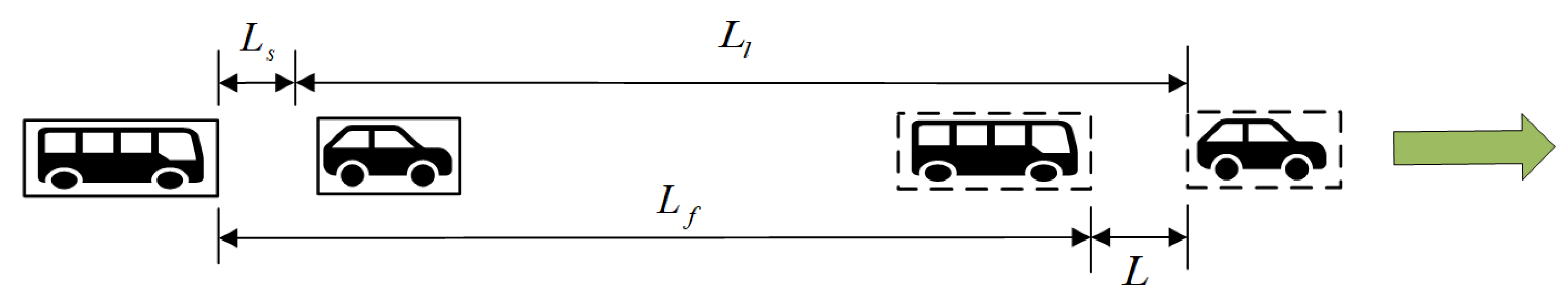
2.2.1. Safe Distance Model

As shown in Figure 2, when vehicles are traveling in the same direction, the prerequisite for a vehicle to accelerate, decelerate, or maintain its current speed is that there is a sufficiently safe distance between it and the vehicle ahead. To avoid collisions, the safety distance must be determined before updating the vehicle’s speed. As shown in Figure 2, the leading and following vehicles are traveling in the same direction. In the case of an emergency, the leading vehicle performs an emergency brake and moves to the position of the dashed line, while the following vehicle also performs an emergency brake in response to the leading vehicle’s deceleration, and finally both vehicles reach the position of the dashed line.

Where $L_f$ represents the braking distance traveled by the following vehicle; $L_l$ represents the braking distance traveled by the leading vehicle; $L$ represents the distance maintained between the following vehicle and the leading vehicle after braking; and $L_s$ represents the safe driving distance. During the emergency braking of a vehicle, the relationship between the various distances can be expressed as follows:

$$L_s=L_f+L-L_l$$

(1)

$$L_l=v_l{t}_l-{\displaystyle \frac{1}{2}}{a}_l{t_l}^2$$

(2)

where $v_l$ is the driving speed before braking of the front vehicle; $t_l$ is the braking time of the front vehicle; $a_l$ is the braking deceleration of the front vehicle. In actual traffic situations, when the driver of the following vehicle notices the brake lights of the leading vehicle turning on and initiates braking, it takes four stages for the vehicle to complete deceleration: driver reaction time $t_r$, vehicle brake coordination time $t_b$, brake force build-up time $t_u$, and continuous braking time $t_c$. The process of decelerating can be expressed as follows:

$$L_f=L_r+L_b+L_u+L_c=v_f(t_r+t_b+t_u+t_c)-{\displaystyle \frac{1}{2}}{a}_f{t}_c^2$$

(3)

where $L_r$ is the braking distance traveled by the trailing vehicle during the driver’s reaction time; $L_b$ is the braking distance traveled by the trailing vehicle during the brake coordination time of the vehicle; $L_u$ is the braking distance traveled by the trailing vehicle during the brake force increase time; $L_c$ is the braking distance traveled by the trailing vehicle during the continuous braking time; $v_f$ is the driving speed of the trailing vehicle before braking; $a_f$ is the braking deceleration of the trailing vehicle.

Based on the above process, we will conduct a detailed analysis of the various distance relationships involved in the car-following process. By substituting Equations (2) and (3) into Equation (1), we obtain the following:

$$L_s=v_f(t_r+t_b+t_u+t_c)-{\displaystyle \frac{1}{2}}{a}_f{t_c}^2+{\displaystyle \frac{1}{2}}{a}_l{t_l}^2-v_l{t}_l+L$$

(4)

However, in actual traffic flow, Equation (4) is not completely accurate. If the acceleration of the two vehicles, such as a heavy-duty truck and a small car, differs due to their inherent performance, the shortest distance between the two vehicles may occur in a state where both vehicles are not stopped. Therefore, for heterogeneous traffic flow consisting of heavy-duty trucks and small cars, it is necessary to consider the change in distance between the two vehicles during each time period as they decelerate to zero speed.

In the literature introduced in Section 1, Introduction, experts and scholars have conducted in-depth research on safety distance models. Therefore, the safety distance model presented in this paper is an extension and application based on existing safety distance models. The safety distance model primarily focuses on vehicle-following and braking processes, and there are three types of driving safety distances: safety distance for accelerating vehicles $L_{sa}$, safety distance for maintaining speed vehicles $L_{sk}$, and safety distance for decelerating vehicles $L_{sd}$. Below, we will analyze the safety distance for accelerating vehicles $L_{sa}$ as an example:

• Assuming at time $t$, the distance between the leading vehicle and the following vehicle is $L_n(t)$, the following vehicle updates its position with a speed of $(v_n(t)+a_n)$. At the same moment, due to a sudden situation, the leading vehicle initiates emergency braking with a deceleration of $E_{n-1}$ and updates its position based on its speed $(v_{n-1}(t)-E_{n-1})$ until it comes to a complete stop. To avoid a rear-end collision, the following vehicle also initiates emergency braking and decelerates until it comes to a complete stop. Assuming that the leading vehicle comes to a stop at time $t+\mathsf{\Delta }{t}_{n-1}$, the following vehicle comes to a stop at time $t+\mathsf{\Delta }{t}_n$ (generally $\mathsf{\Delta }{t}_{n-1}\ne \mathsf{\Delta }{t}_n$), and during the process of emergency braking until both vehicles come to a complete stop, they just barely avoid a collision. Based on the above analysis, the distance $L_n(t)$ between the two vehicles at time $t$ represents the critical safety distance $L_{sa}$ for the following vehicle to decelerate safely. This critical safety distance $L_{sa}$ can be calculated.

Assuming that both the vehicle in front and the vehicle behind have ceased moving at time $t+\mathsf{\Delta }t$, then

$$\mathsf{\Delta }t=\mathit{max}\left(\mathsf{\Delta }{t}_{n-1},\mathsf{\Delta }{t}_n\right)$$

(5)

Between the time $t$ and the time $t+\mathsf{\Delta }t$, the cumulative driving distances of the leading vehicle and the trailing vehicle within each time step $t+j$ are summed up, and the calculation expression is as follows:

$$L_l\left(j\right)={\displaystyle \sum _{i=0}^j\left[\mathit{max}\left(0,v_{n-1}(t)-E_{n-1}-i{E}_{n-1}\right)\right]}$$

(6)

$$L_f\left(j\right)=L_r+L_b+L_u+{\displaystyle \sum _{i=0}^j\left[\mathit{max}\left(0,v_n(t)+a_n-i{E}_n\right)\right]}$$

(7)

among them, $j$ = 0, 1, 2, $\mathsf{\Delta }t$.

According to the definition, the maximum difference between the cumulative driving distances of the following vehicle and the preceding vehicle is the critical safe distance, and its expression is as follows:

$$L_{sa}\left(t\right)=\mathit{max}\left(L_f(j)-L_l(j)\right)$$

(8)

From the above formula, we can obtain that

$$L_{sa}\left(t\right)=\mathit{max}\left\{\begin{array}{l}{L}_r+L_b+L_u+{\displaystyle \sum _{i=0}^j\left[\mathit{max}\left(0,v_n(t)+a_n-i{E}_n\right)\right]}-\\ {\displaystyle \sum _{i=0}^j\left[\mathit{max}\left(0,v_{n-1}(t)-E_{n-1}-i{E}_{n-1}\right)\right]}\end{array}\right\}$$

(9)

For the convenience of subsequent descriptions in this paper, we define the expression for $L_{sa}(t)$ as follows:

$$L_{sa}\left(t\right)=f\left(L_r,L_b,L_u;v_n(t)+a_n,E_n;v_{n-1}(t)-E_{n-1},E_{n-1}\right)$$

(10)

Therefore, when the distance between the following vehicle and the leading vehicle satisfies the condition $L_n(t)$ ≥ $L_{sa}(t)$, the following vehicle can accelerate; when $L_n(t)$ < $L_{sa}(t)$, to prevent a collision, the following vehicle should not accelerate.

2.

The calculation process for the safe distance $L_{sk}$ when a car maintains its speed is similar to that for the safe distance $L_{sa}$ when a car accelerates. The difference lies in that, at time $t$, the position of the car behind is updated based on its current speed $v_n(t)$. By analogy to the calculation process of $L_{sd}(t)$, we can derive the expression for $L_{sk}(t)$ as follows:

$$L_{sk}\left(t\right)=f\left(L_r,L_b,L_u;v_n(t),E_n;v_{n-1}(t)-E_{n-1},E_{n-1}\right)$$

(11)

Therefore, when the distance between the following vehicle and the leading vehicle satisfies the condition $L_{sk}(t)$ ≤ $L_n(t)$ < $L_{sa}(t)$, the following vehicle can maintain its current speed; when $L_n(t)$ < $L_{sk}(t)$, in order to avoid a collision, the following vehicle needs to decelerate.

3.

Similarly, the calculation process for the safe distance $L_{sd}$ when a car decelerates is analogous to that for the safe distance $L_{sa}$ when a car accelerates and the safe distance $L_{sk}$ when a car maintains its speed. The difference lies in that, at time $t$, the position of the following car is updated based on its speed $(v_n(t)-a_n)$. By analogy to the calculation processes of $L_{sa}(t)$ and $L_{sk}(t)$, we can derive the expression for $L_{sd}(t)$ as follows:

$$L_{sd}\left(t\right)=f\left(L_r,L_b,L_u;v_n(t)-a_n,E_n;v_{n-1}(t)-E_{n-1},E_{n-1}\right)$$

(12)

Therefore, when the distance between the following vehicle and the leading vehicle satisfies the condition $L_{sd}(t)$ ≤ $L_n(t)$ < $L_{sk}(t)$, the following vehicle needs to decelerate, whereas when $L_n(t)$ < $L_{sd}(t)$, in order to avoid a collision, the following vehicle needs to perform emergency braking.

2.2.2. Car-Following Rule

Based on the previously mentioned safe distance model, during the transition from time $t$ to $t$ + 1, an improved car-following rule is established by evaluating the relationship between the vehicle spacing $L_n(t)$ and the three types of safe distances. The cellular automaton model based on safe distances evolves according to the following rules.

1.

Acceleration:

At time t, if the distance between a vehicle and the preceding vehicle is not less than the critical safe distance for acceleration and the vehicle’s speed is less than the maximum speed, the vehicle accelerates; if the distance is less than the critical safe distance for acceleration but not less than the critical safe distance for maintaining speed, the vehicle maintains its current speed.

$$v_n(t+1)=\left\{\begin{array}{l}\mathit{min}\left(v_n(t)+a_n,v\mathit{max}\right),L_n(t)\ge L_{sa}(t)\\ v_n(t),L_{sk}(t)\le L_n(t)<L_{sa}(t)\end{array}\right.$$

(13)

2.

Deceleration:

(1) At time $t$, when a vehicle is relatively far away from the intersection (with $S_n$ not less than 5 cells) and the distance to the preceding vehicle is less than the critical safe distance for maintaining speed but not less than the critical safe distance for decelerating, the vehicle decelerates; when the distance is less than the critical safe distance for decelerating, the vehicle applies emergency braking.

$$v_n\left(t+1\right)=\left\{\begin{array}{l}\mathit{max}\left(v_n(t)-a_n,0\right),L_{sd}(t)\le L_n(t)<L_{sk}(t)\\ \mathit{max}\left(v_n(t)-a_{nm},0\right),L_n(t)<L_{sd}(t)\end{array}\right.$$

(14)

(2) At time $t$, when a vehicle is relatively close to the intersection (with $S_n$ less than 5 cells) and the distance to the preceding vehicle is not less than the critical safe distance for decelerating, the vehicle decelerates; when the distance is less than the critical safe distance for decelerating, the vehicle applies emergency braking.

Scenario I: When the intersection traffic light is green.

In Scenario I, $v_n\to \mathit{min}(v_n,L_n,S_n+1)$ indicates that the vehicle needs to decelerate as it passes through the intersection. The maximum speed within the intersection is 1 cell/s, meaning that when the vehicle enters the intersection from the roadway, it can only advance to the first cell within the intersection in its first step.

Scenario II: When the intersection traffic light is red.

① Straight-moving and left-turning vehicles: $v_n\to \mathit{min}(v_n,L_n,S_n)$, indicating that straight-moving and left-turning vehicles are stopped due to the red light.

② Right-turning vehicles: $v_n\to \mathit{min}(v_n,L_n,S_n)$ when they are controlled by signals; $v_n\to \mathit{min}(v_n,L_n,S_n+1)$ when they are not controlled by signals.

3.

Random Slowdown:

If a vehicle that decelerated in the previous step undergoes random slowdown in this step, its speed will decrease by 2$a_n$ within one time step, which exceeds the vehicle’s deceleration capability. Therefore, random slowdown is only applied to vehicles that did not experience deceleration in the previous step.

$$v_n\left(t+1\right)=\mathit{max}\left(v_n(t)-a_n,0\right)\left\{\begin{array}{l}rand<R\\ L_n(t)\ge L_{sa}(t)\end{array}\right.$$

(15)

where $rand$ is the randomization number for slowdown, and $R$ is the probability of a random slowdown.

4.

Location Update.

$$x_n\left(t+1\right)=x_n\left(t\right)+v_n\left(t+1\right)$$

(16)

2.2.3. Lane-Changing Rules

This article categorizes lane-changing rules into rational lane changing and forced lane changing. Rational lane changing refers to the behavior of a vehicle changing lanes without affecting the following vehicle in the target lane, whereas forced lane changing may cause the following vehicle in the target lane to decelerate.

• Rational Lane-Changing Rules: When the target vehicle cannot travel at its maximum speed in the current lane and cannot accelerate and there is sufficient distance in the target lane for acceleration without affecting the following vehicle in that lane, then a rational lane change is performed.

$$v_n\left(t\right)<v_{\mathit{max}}\left(t\right),L_n\left(t\right)<L_{sa}\left(t\right)$$

(17)

$$L_{n,front}\left(t\right)\ge L_{sa,fornt}\left(t\right),L_{n,back}\left(t\right)\ge L_{sk,back}\left(t\right)$$

(18)

where $L_{sa,fornt}\left(t\right)$ is the critical safe distance for the vehicle to accelerate in the target lane, and $L_{sk,back}\left(t\right)$ is the critical safe distance for the following vehicle in the target lane to maintain its speed.

2.

Forced Lane-Changing Rules: When the target vehicle cannot travel at its maximum speed in the current lane and cannot accelerate, but there is sufficient distance in the target lane for acceleration, which may cause the following vehicle in that lane to decelerate but not to perform emergency braking, then a forced lane change is performed.

$$v_n\left(t\right)<v_{\mathit{max}}\left(t\right),L_n\left(t\right)<L_{sa}\left(t\right)$$

(19)

$$L_{n,front}\left(t\right)\ge L_{sa,fornt}\left(t\right),L_{sd,back}\left(t\right)\le L_{n,back}\left(t\right)<L_{sk,back}\left(t\right)$$

(20)

where $L_{sd,back}\left(t\right)$ represents the critical safe distance for the following vehicle in the target lane to decelerate.

2.3. Rules for Updating Vehicles at Intersections

The cellular division and vehicle trajectories at the intersection are shown in Figure 3. The cells at the intersection are divided into two types: (1) outer intersection cells (cells 1 to 12); (2) inner intersection cells (cells 13 to 16). Vehicles traveling straight, turning left, and turning right follow different trajectories to cross the intersection. For example, left-turning vehicles on Lane 1 enter Lane 5 along the path of cells 5-14-13-16-9; vehicles traveling straight can proceed directly along the path of cells 5-14-13-12; and right-turning vehicles enter Lane 8 via cell 4. The vehicles on the remaining lanes follow the same updating rules. Within the intersection, the speed of vehicles can be either 0 or 1. At the intersection, the position update of vehicles follows the car-following rules and intersection traffic rules established in this paper. Vehicles determine their speed for the next time step as either 0 or 1 based on these rules and then move forward accordingly, updating their cell position along the route. After the position update, the original cell occupied by the vehicle becomes vacant, while the new cell where the vehicle is located becomes occupied.

This study establishes the traffic rules for signal-controlled intersections as follows: the through and left-turn movements in the north–south direction constitute one phase, and the through and left-turn movements in the east–west direction constitute another phase. In the event of a conflict between a left-turn and a through movement, priority is given to the through movement, with alternating passage. Taking a left-turning vehicle from east to south as an example, if a vehicle on Lane 1 occupies cell 13 and intends to turn left onto Lane 5 via cell 16, while a vehicle on Lane 3 occupies cell 11 and intends to continue straight ahead via cell 16, a conflict will arise at cell 16 between the two vehicles. According to the intersection traffic rules established in this study, the through vehicle on Lane 3 will be allowed to proceed and occupy cell 16 on a priority basis, provided that a safe distance is maintained from the preceding vehicle. The left-turning vehicle on Lane 1 will then enter cell 16 after the through vehicle has passed. Subsequently, vehicles on the two lanes will alternately occupy cell 16 to cross the intersection. If cell 13 is unoccupied or occupied by a through vehicle on Lane 1, there is no conflict with the through vehicle on Lane 3, and the latter may pass through the intersection without considering the priority or alternating passage rules, as long as a safe distance is maintained. Similarly, if cell 11 is unoccupied, the left-turning vehicle on Lane 1 may also pass through the intersection without considering the priority or alternating passage rules, as long as a safe distance is maintained.

3. Simulation Setup and Result Analysis

3.1. Setting of Cellular Parameters

This study utilizes a self-built simulation environment in Python 3.10, which includes a cellular automaton model, a parameter configuration file, a method for visualizing simulation results, and a main simulation execution program. The cellular automaton model is used to define the road environment, vehicle update rules, and other environmental factors, as well as to record simulation data. The parameter configuration file is used to set various parameters for the cellular simulation. The method for visualizing simulation results is used to display the simulation outcomes visually. The main simulation execution program is responsible for invoking the aforementioned files to run the simulation and output the results.

The simulation environment consists of an arterial road and several access roads, all of which are two-way four-lane urban roads. Each road is modeled with a length of 1000 cells, with each cell measuring 5 m in length. Small cars have a length of 1 cell (5 m), while heavy-duty vehicles occupy a length of 2 cells (10 m). The maximum speed for small cars is 5 cells (25 m/s), with an initial speed of 3 cells (15 m/s). For heavy-duty vehicles, the maximum speed is 3 cells (15 m/s), and the initial speed is 2 cells (10 m/s). Among them, the signal-controlled intersection has a total of two phases. The arterial road runs in the east–west direction, while the access road runs in the north–south direction. Right-turning vehicles are not controlled by signals. In the first phase, the green light duration for straight and left-turn movements in the east–west direction is 38 s. In the second phase, the green light duration for straight and left-turn movements in the north–south direction is 17 s. The duration of the yellow light is 4 s, and the all-red time is 2 s. The probabilities for vehicles to travel straight and turn right in each direction are 0.8 and 0.2, respectively, while the random deceleration probability for vehicles is 0.02. To facilitate the control of the traffic flow density, the simulation adopts periodic boundary conditions, meaning that vehicles exiting from the end of the road will re-enter the lane from the beginning of the road. For each vehicle type configuration and each traffic flow density, the simulation runs for 1000 time steps. During the simulation process, the average values of various traffic flow parameters are calculated every 20 time steps.

3.2. Analysis of the Impact of Heavy-Duty Vehicles on Traffic Flow

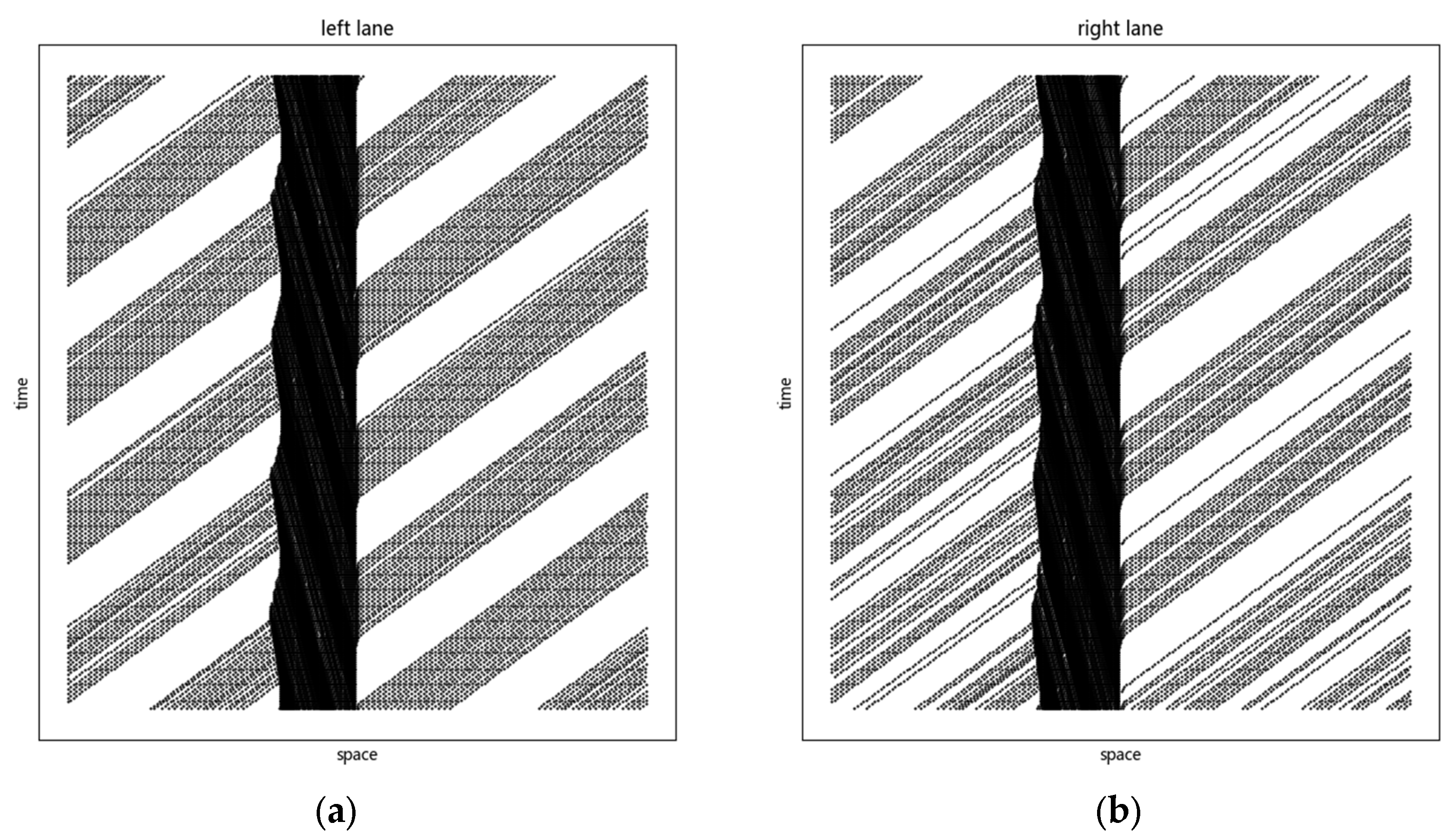
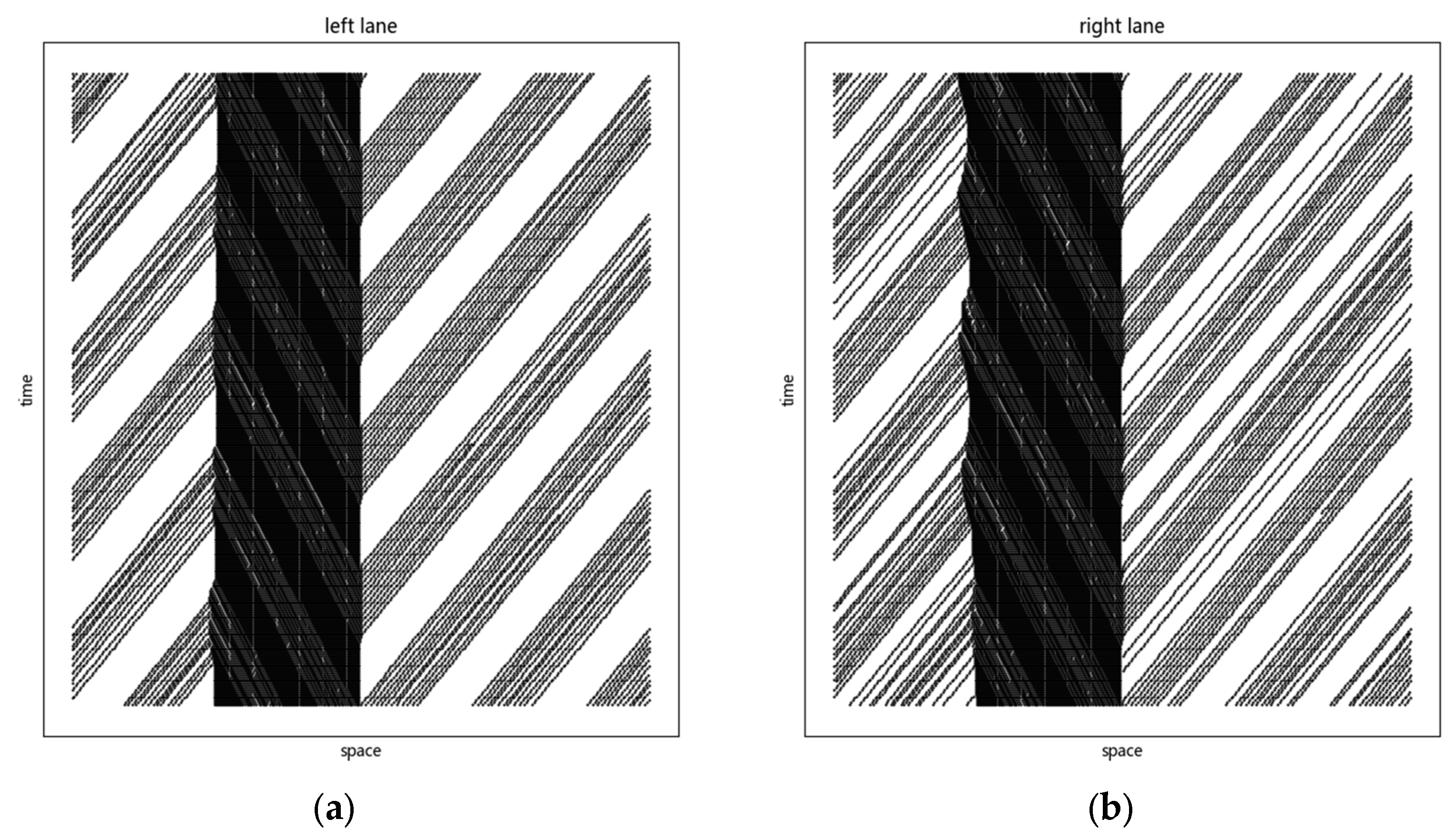
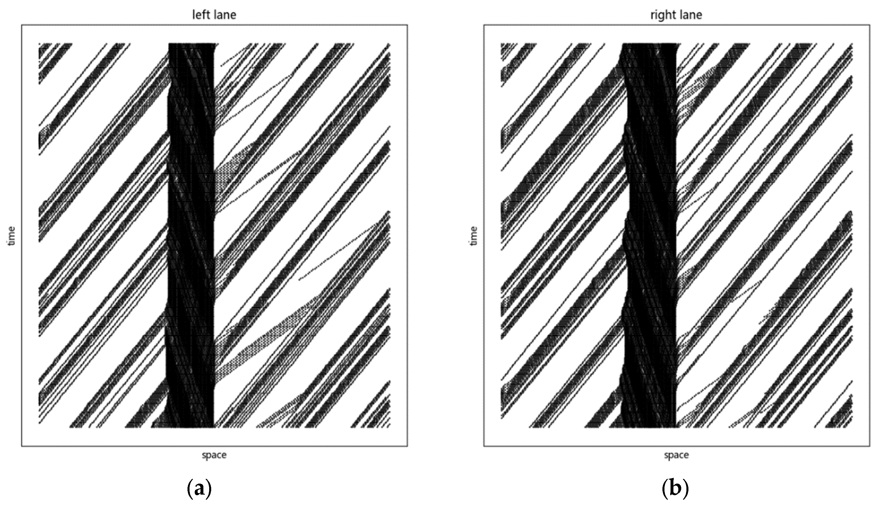
3.2.1. Analysis of Spatial-Temporal Operation Diagrams

As shown in Figure 4, a spatial-temporal operation chart is a graphical representation method that cleverly exhibits the movement trajectories of vehicles across two dimensions: time as the vertical axis and space as the horizontal axis. This study aims to visually present the vehicle movement in model simulations through spatial-temporal charts. Specifically, it precisely records the position information of all vehicles on a certain lane at each time step and plots this information as scatter points on the spatial-temporal operation chart. In the chart, the vertical axis clearly represents the progression of time, with each vertical line perpendicular to it corresponding to a specific time step, showcasing the spatial distribution of all vehicles on the lane at that time step. The horizontal axis, on the other hand, represents the spatial positions along the lane, with each vertical line perpendicular to it corresponding to a specific cell on the lane, indicating the occupancy of that cell by vehicles at different time steps. The concept of cell space is crucial in spatial-temporal operation charts, representing the small spatial units into which the lane is divided. Each point in the chart corresponds to the state where a certain cell is occupied by a vehicle at a specific time step. Notably, the blank areas in the chart explicitly indicate that a particular cell is not occupied by any vehicle at a given time step. By observing the density of scatter points in the spatial-temporal operation chart, we can intuitively capture key information about the traffic flow. For example, densely populated areas often represent traffic congestion points, while the transition from dense to sparse scatter points vividly illustrates the formation and dissipation of traffic bottlenecks. To facilitate observation and reading, this study carefully selects the cell space near intersections along the road segment for plotting. This approach not only focuses the spatial-temporal operation chart on critical areas of the traffic flow but also provides a powerful visual aid for an in-depth understanding and analysis of traffic phenomena.

By comparing the spatial-temporal operation diagrams when the proportion of heavy-duty vehicles is 0 and 1, it can be observed that when the road network is entirely composed of heavy-duty vehicles, the average speed of the road network is much slower than that of a road network composed entirely of small vehicles from Figure 4 and Figure 5. A commonality between these two scenarios is that the vehicle trajectories are relatively smooth, and there is no crossing or overlapping between the curves, indicating that when only one type of vehicle exists on a road segment, vehicles can achieve coordinated car-following based on the distance to the preceding vehicle, and there is no occurrence of rear-end collisions during the car-following process.

By setting the proportion of heavy-duty vehicles in the road network traffic flow to 0.3, the formation process of moving bottlenecks becomes clearly visible from Figure 6. Small vehicles, influenced by heavy-duty vehicles, decelerate after accelerating and can only follow at low speeds behind the heavy-duty vehicles, unable to further accelerate. Meanwhile, the lane-changing behaviors of vehicles can be clearly observed in the spatial-temporal diagram, where the vehicle trajectories are no longer complete and continuous curves. The discontinuity in the trajectory lines in the diagram represents vehicles changing lanes to merge into or exit from the current lane. The above analysis demonstrates that this model can truly reflect car-following and lane-changing behaviors, achieving the expected simulation effects.

3.2.2. The Impact of the Proportion of Heavy-Duty Vehicles on Traffic Flow

From Figure 7, it can be observed that the average traffic flow rate per lane is maximized when the traffic stream consists solely of small cars, with the maximum flow rate being approximately 950 vehicles per hour (veh/h). Conversely, when the proportion of heavy-duty trucks is 0.4, the average traffic flow per lane is minimum, with a maximum flow rate of approximately 850 veh/h. As the input traffic density increases, the volume of traffic passing through the intersection also grows. At this point, the total number of vehicles on the road is increasing but has not yet exceeded the road’s traffic capacity. When the traffic density reaches a certain level, the growth rate of traffic flow at the intersection gradually slows down and even exhibits a downward trend. This phenomenon is more pronounced in simulations where the proportion of heavy vehicles in the input traffic is higher. The larger the proportion of heavy vehicles, the sooner the traffic flow decline occurs. The reason for the above situation is that compared to small vehicles, heavy-duty vehicles occupy more cells and require more road space, resulting in lower driving flexibility. As the proportion and number of heavy-duty vehicles increase, the actual traffic capacity of the road decreases, forcing small vehicles to travel at lower speeds. The above analysis indicates that under the same traffic density, a larger proportion of heavy-duty vehicles in the traffic flow will lead to a decrease in the actual road capacity, which aligns with phenomena observed in actual road traffic.

3.2.3. Impact of the Proportion of Heavy-Duty Vehicles on Vehicle Speed

From Figure 8, it can be observed that the average vehicle speed is maximized when only small cars are present in the traffic flow, while it is minimized when the proportion of heavy-duty trucks is 0.4. As the input traffic density increases, the average speed of the road network’s traffic flow gradually decreases, but the rate of decline gradually flattens out. When the traffic flow density (k) of the road network is less than 80 vehicles per kilometer (veh/km), the proportion of heavy-duty vehicles has a significant impact on the average speed of the traffic flow. With a constant traffic flow density, the average speed decreases as the proportion of heavy-duty trucks increases. However, when the traffic flow density (k) exceeds 80 vehicles per kilometer (veh/km), the influence of the proportion of heavy-duty vehicles on the average speed becomes less pronounced. These results indicate that when the traffic density is low, the introduction of heavy-duty vehicles restricts the speed of following vehicles in the same lane, forcing them to decelerate, follow at a distance, or change lanes to maintain a safe distance between vehicles. At this point, the moving bottleneck effect is evident. However, as the traffic density increases and road traffic approaches saturation, the impact of heavy-duty vehicles on traffic flow diminishes, and the moving bottleneck effect weakens.

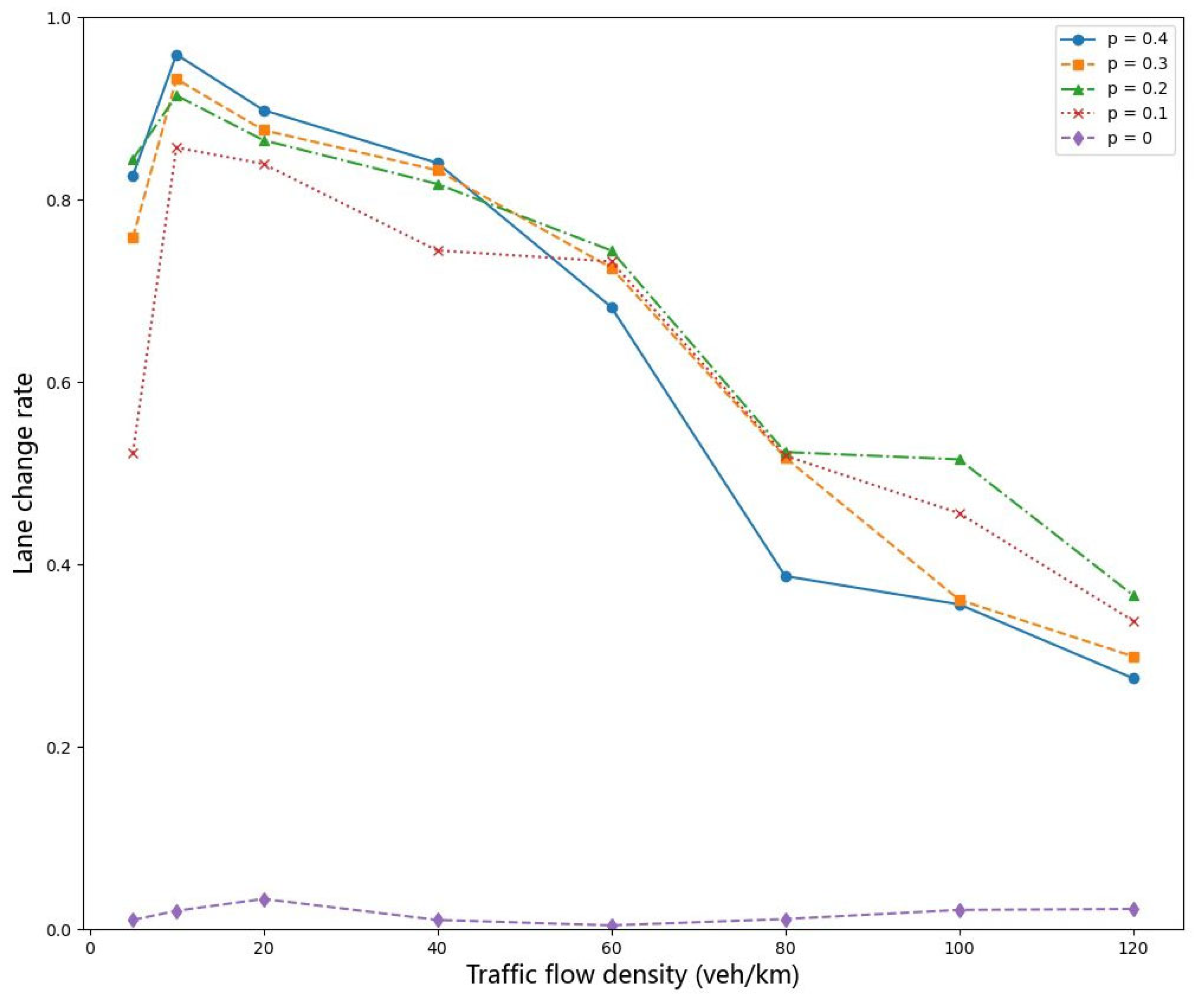
3.2.4. Impact of Heavy-Duty Vehicle Proportion on Lane-Changing Rate

From Figure 9, it can be observed that when the density ρ is less than or equal to 45 vehicles per kilometer (veh/km), under the condition of constant traffic density, the lane-changing rate of small cars increases as the proportion of heavy-duty vehicles increases. This is due to the fact that a higher proportion of heavy-duty vehicles creates a more significant moving bottleneck effect, which subsequently increases the lane-changing demand for small cars. Additionally, in low-density conditions, the road space does not undergo significant changes with the increase in the number of heavy-duty vehicles, allowing small cars, even after being affected by heavy-duty vehicles, to still have sufficient space for lane changing. When ρ is greater than 45 vehicles per kilometer (veh/km), under the condition of constant traffic density, the lane-changing rate of small cars decreases as the proportion of heavy-duty vehicles increases. This is because when the traffic density is sufficiently high, as the proportion of heavy-duty vehicles increases, the space they occupy becomes larger and larger, causing the gaps between vehicles on the road to shrink, which in turn makes it increasingly difficult for small cars to change lanes.

4. Conclusions

This paper presents a two-lane cellular automaton model suitable for simulating urban road traffic that includes intersections, based on the NaSch model. The model comprehensively considers multiple key factors, such as the vehicle safety distance, speed differences between adjacent vehicles, acceleration and deceleration performance of different vehicle types, and driver reaction time, enabling it to more realistically reproduce the complex characteristics of mixed traffic flow on urban roads. Currently, research in this field is relatively scarce both domestically and internationally, and the proposal of this model makes a certain contribution to the field. Furthermore, subsequent research can be further expanded on this basis, applying the model to more complex road scenarios, such as three-lane and four-lane roads. At the same time, the vehicle update rules at intersections can also be flexibly extended based on this model, making it adaptable to the actual road traffic conditions of different countries and cities, demonstrating strong applicability and scalability. This paper focuses on studying and analyzing the impact of the traffic flow density and the proportion of heavy-duty vehicles on the moving bottleneck effect in urban roads, from the aspects of spatial–temporal evolution diagrams, the traffic flow volume, average speeds, and lane-changing rates. The results indicate the following: (1) in the traffic flow state where heavy and small vehicles are mixed, the lane-changing behavior of vehicles is particularly evident in the spatial–temporal diagrams, and the formation process of moving bottlenecks is clearly demonstrated. The model established in this paper successfully simulates the characteristics of urban road mixed traffic flow. The simulation results are highly consistent with actual traffic conditions, achieving the expected simulation effects and possessing practical application value. (2) The higher the proportion of heavy-duty vehicles on urban roads, the stronger the moving bottleneck effect. This confirms the necessity of conducting research on the phenomena of moving bottlenecks and the traffic impact mechanisms on urban roads. (3) Based on the research in this paper, further in-depth studies will be conducted in two areas: firstly, studying the traffic flow characteristics of mixed traffic with multiple vehicle types moving at different speeds on urban roads, especially in special scenarios, such as the coexistence of autonomous and human-driven vehicles; secondly, exploring the use of platoon control methods to mitigate the moving bottleneck phenomenon on urban roads.

References

1. Gazis, D.C.; Herman, R. The moving and ‘phantom’ bottleneck. Transp. Sci. 1992, 26, 223–229. [Google Scholar] [CrossRef]
2. Newell, G.F. A moving bottleneck. Transp. Res. Part B 1998, 32, 53l–537. [Google Scholar] [CrossRef]
3. Lebacque, J.P.; Lesort, J.B.; Giorgi, F. Introducing buses in first order traffic flow models. Transp. Res. Rec. 1998, 1644, 70–79. [Google Scholar] [CrossRef]
4. Yang, X.F.; Fu, Q. Research Progress in Moving Bottleneck Theory. Comput. Eng. Appl. 2011, 47, 1–3. [Google Scholar] [CrossRef]
5. Piacentini, G.; Goatin, P.; Ferrara, A. Traffic control via moving bottleneck of coordinated vehicles. IFAC Pap. OnLine 2018, 51, 13–18. [Google Scholar] [CrossRef]
6. Xu, J.M.; Yang, Z.B.; Ma, Y.Y. Research on Expressway Traffic Flow Control Model for Moving Bottlenecks. J. Guangxi Norm. Univ. Nat. Sci. Ed. 2020, 38, 10. [Google Scholar] [CrossRef]
7. Li, Z.; Levin, M.W.; Stem, R.; Que, X. A network traffic model with controlled autonomous vehicles acting as moving bottlenecks. In Proceedings of the 2020 IEEE 23rd International Conference on Intelligent Transportation Systems (ITSC), Rhodes, Greece, 20–23 September 2020. [Google Scholar] [CrossRef]
8. Li, Q.F. Research on Traffic Flow Problems Based on Multi-lane Moving Bottlenecks. Master’s Thesis, Lanzhou Jiaotong University, Lanzhou, China, 2021. [Google Scholar] [CrossRef]
9. Hu, X.; Lin, C.; Hao, X.; Lu, R.; Liu, T. Influence of tidal lane on traffic breakdown and spatiotemporal congested patterns at moving bottleneck in the framework of Kerner’s three-phase traffic theory. Phys. A Stat. Mech. Its Appl. 2021, 584, 126335. [Google Scholar] [CrossRef]
10. Goatin, P.; Daini, C.; Monache, M.D.; Ferrara, A. Interacting moving bottlenecks in traffic flow. Netw. Heterog. Media 2023, 18, 930–945. [Google Scholar] [CrossRef]
11. Laarej, A.; Lakouari, N.; Karakhi, A.; Ez-Zahraouy, H. Analyzing the effect of fixed and moving bottlenecks on traffic flow and car accidents in a two-lane cellular automation model. J. Appl. Eng. Sci. 2023, 21, 1158, 1179–1191. [Google Scholar] [CrossRef]
12. Liu, H.Q.; Jiang, R. Efficient control of connected and automated vehicles on a two-lane highway with a moving bottleneck. Chin. Phys. B 2023, 32, 054501. [Google Scholar] [CrossRef]
13. Li, X.; Xiao, Y.; Jia, B. Modeling mechanical restriction differences between car and heavy truck in two-lane cellular automata traffic flow model. Phys. A Stat. Mech. Its Appl. 2016, 451, 49–62. [Google Scholar] [CrossRef]
14. Wang, K. Research on Moving Bottlenecks of Heavy-Duty Trucks on Expressways Based on Cellular Automata. Master’s Thesis, Huazhong University of Science and Technology, Wuhan, China, 2017. [Google Scholar] [CrossRef]
15. Pan, W.; Chen, X.; Duan, X. Energy dissipation and particulate emission at traffic bottleneck based on NaSch model. Eur. Phys. J. B Condens. Matter 2022, 95, 105. [Google Scholar] [CrossRef]
16. Shang, X. Lane-changing behavior modeling and traffic flow characteristics analysis based on cellular automaton. PhD Thesis, Beijing Jiaotong University, Beijing, China, 2023. [Google Scholar] [CrossRef]
17. Gong, B.; Wang, F.; Lin, C.; Wu, D. Modeling HDV and CAV Mixed Traffic Flow on a Foggy Two-Lane Highway with Cellular Automata and Game Theory Model. Sustainability 2022, 14, 5899. [Google Scholar] [CrossRef]
18. Gui, S.R.; Lan, T.F.; Chen, S.S.; Ge, S.Q. Research on a Traffic Flow Model Considering Vehicle Heterogeneity in Congested Conditions. Complex Syst. Complex. Sci. 2023, 20, 98–104. [Google Scholar] [CrossRef]
19. Masaka, J.; Sueyoshi, F.; Hossain, M.A.; Utsumi, S.; Tanimoto, J. Can the introduction of CAVs mitigate social dilemmas causing traffic jams on highways? Phys. Open 2023, 17, 100176. [Google Scholar] [CrossRef]
20. Wang, Z.; Chen, T.; Wang, Y.; Li, H. A cellular automaton model for mixed traffic flow considering the size of CAV platoon. Phys. A Stat. Mech. Appl. 2024, 643, 129822. [Google Scholar] [CrossRef]
21. Li, S.; Yanagisawa, D.; Nishinari, K. A jam-absorption driving system for reducing multiple moving jams by estimating moving jam propagation. Transp. Res. Part C Emerg. Technol. 2024, 158, 104394.1–104394.25. [Google Scholar] [CrossRef]
22. Wang, X.; Zeng, J.; Qian, Y.; Wei, X.; Zhang, F. Heterogeneous traffic flow of expressway with Level 2 autonomous vehicles considering moving bottlenecks. Phys. A Stat. Mech. Appl. 2024, 650, 129991. [Google Scholar] [CrossRef]
23. Li, S.L.; Zhang, X.D.; Shi, J.Q.; Zhang, L. Modeling and Capacity Analysis of Traffic Flow at Signal-Controlled Intersections. J. Highw. Transp. Res. Dev. 2017, 34, 7. [Google Scholar] [CrossRef]
24. Ez-Zahar, A.; Lakouari, N.; Oubram, O.; Marzoug, R.; Ez-Zahraouy, H. Analyzing single-lane roundabout traffic and environmental impacts through cellular automaton: A focus on U-turn effects. Int. J. Mod. Phys. C Comput. Phys. Phys. Comput. 2024, 35, 2450114. [Google Scholar] [CrossRef]
Figure 1. A scheme of the road network.
Applsci 15 03547 g001
Figure 2. Illustration of vehicle-following process.
Applsci 15 03547 g002
Figure 3. Schematic diagram of intersection.
Applsci 15 03547 g003
Figure 4. (a,b) Spatial-temporal operation diagram when the proportion of heavy-duty vehicles is 0.
Applsci 15 03547 g004
Figure 5. (a,b) Spatial-temporal operation diagram when the proportion of heavy-duty vehicles is 1.
Applsci 15 03547 g005
Figure 6. (a,b) Spatial-temporal operation diagram when the proportion of heavy-duty vehicles is 0.3.
Applsci 15 03547 g006
Figure 7. Traffic flow volume–density diagram.
Applsci 15 03547 g007
Figure 8. Traffic flow speed–density diagram.
Applsci 15 03547 g008
Figure 9. Traffic flow lane-changing rate—density diagram.
Applsci 15 03547 g009
Disclaimer/Publisher’s Note: The statements, opinions and data contained in all publications are solely those of the individual author(s) and contributor(s) and not of MDPI and/or the editor(s). MDPI and/or the editor(s) disclaim responsibility for any injury to people or property resulting from any ideas, methods, instructions or products referred to in the content.