Abstract
Maximizing the energy output of photovoltaic (PV) systems is becoming increasingly important. Consequently, numerous approaches have been developed over the past few years that utilize remote sensing data to predict or map solar potential. However, they primarily address hypothetical scenarios, and few focus on improving existing installations. This paper presents a novel method for optimizing the tilt angles of existing PV arrays by integrating Very High Resolution (VHR) satellite imagery and airborne Light Detection and Ranging (LiDAR) data. At first, semantic segmentation of VHR imagery using a deep learning model is performed in order to detect PV modules. The segmentation is refined using a Fine Optimization Module (FOM). LiDAR data are used to construct a 2.5D grid to estimate the modules’ tilt (inclination) and aspect (orientation) angles. The modules are grouped into arrays, and tilt angles are optimized using a Simulated Annealing (SA) algorithm, which maximizes simulated solar irradiance while accounting for shadowing, direct, and anisotropic diffuse irradiances. The method was validated using PV systems in Maribor, Slovenia, achieving a 0.952 F1-score for module detection (using FT-UnetFormer with SwinTransformer backbone) and an estimated electricity production error of below 6.7%. Optimization results showed potential energy gains of up to 4.9%.
1. Introduction
Solar energy harvesting plays a significant role in renewable energy production, particularly in the past decade, due to the decreasing costs of photovoltaic (PV) modules, green energy initiatives, and the increased nominal power output of PV technologies [1]. Modules are a popular choice for solar energy harvesting, suitable not just for large-scale PV systems but also for smaller installations on building rooftops in urban environments [2].
Over the past few years, a number of simulation and machine learning methods have been developed to accurately estimate the viability of rooftops for PV systems’ placement. The increased availability in remote sensing data, such as Light Detection and Ranging (LiDAR), provides a more accurate 3D representation of building rooftops and their surroundings. This helps to better incorporate the effects of shading, especially in dense urban contexts. Airborne LiDAR scanning involves an aircraft emitting a laser pulse, which is reflected back to the aircraft. The time taken for the pulse to travel allows the estimation of the distance to the surface, resulting in a 3D point cloud [3]. Over the years, various methods have been developed that utilize point cloud data derived from LiDAR or an unmanned aerial vehicle (UAV) to assess the solar or PV potential of 3D surfaces using solar irradiance simulation or deep learning approaches [4,5,6,7]. Moreover, newer methods leverage 3D surface information for the optimal placement of hypothetical PV systems [8,9].
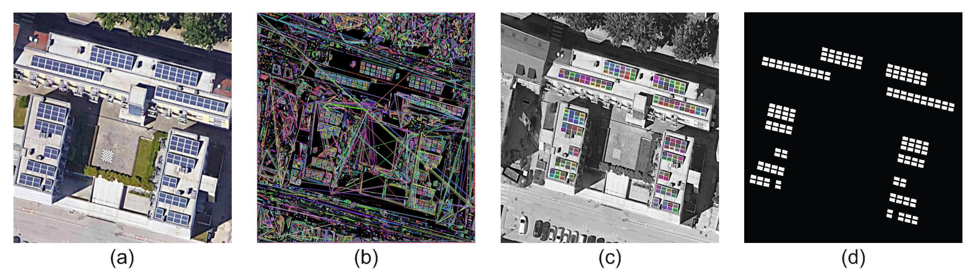
In addition to airborne LiDAR data, very high-resolution (VHR) satellite or aerial imagery, with a resolution of less than 1 m2 per pixel, is already widely available for many geographic areas. Consequently, methods have been developed to identify the installations of existing PV systems in both lower and higher resolutions [10]. When dealing with PV detection in VHR, there can be three levels of granularity involved, as seen in Figure 1, where an entire PV system can be detected (Figure 1b), individual PV arrays (Figure 1c) or individual PV modules (Figure 1d). In recent years, various methods have been developed to perform semantic segmentation using convolutional neural networks (CNNs) [11,12]. Chen et al. [13] have demonstrated that classical machine learning delivers high-quality results when dealing with low-resolution satellite imagery, while Li et al. [14] have shown that the detection of arrays and modules in VHR is more challenging due to class imbalance, non-concentrated distribution, homogeneous texture, and heterogeneous color features. Hence, more recent works primarily employ U-shaped encoder–decoder deep learning architectures such as classical U-Net derivations [11]; a modified CNN pipeline with U-Net [15] using ResNet50 encoding [16]; a cross-learning-driven U-Net [17]; a modified U-Net with VGG16 encoding [18]; a self-paced residual aggregated network [19]; a split-attention network combined with a dual-attention network [20]; coarse prediction with fine optimization [21]; various U-Nets with EfficientNet [22], SE-ResNeXt [23], and InceptionResNet [24] backbone encoders [25]; and recently using a vision Transformer [26]. All of the aforementioned methods focus on the detection of entire PV systems (low granularity) or arrays (medium granularity). Only a few attempts are made in the literature for the detection of individual modules [27], where the best results were obtained utilizing scarcely available remote sensing data, such as hyperspectral [28] or thermal imagery [29], without considering optical VHR imagery or LiDAR data.
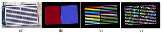
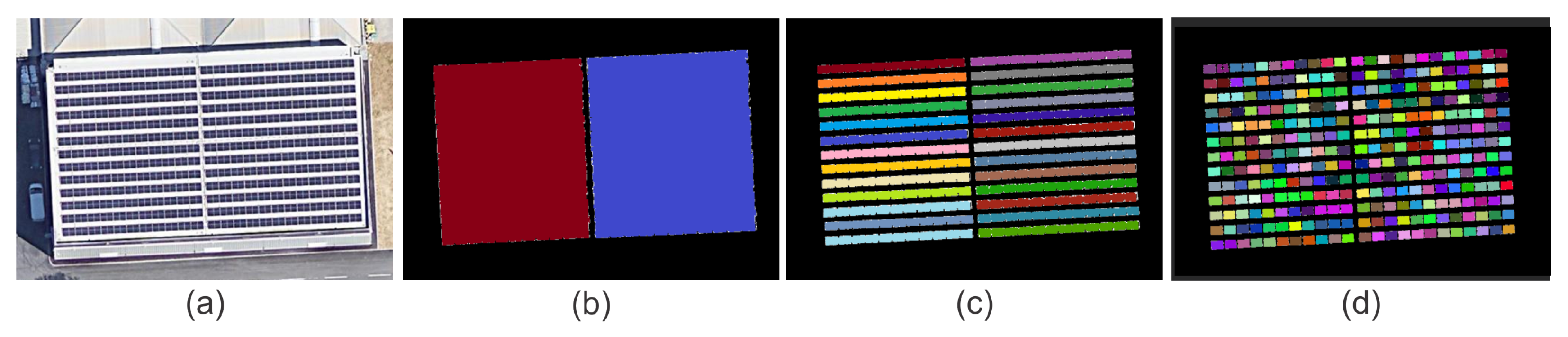
Figure 1.
Example VHR imagery of two PV systems, where (a) is the raw color image, where various methods can detect either (b) PV systems (low granularity), (c) individual PV arrays (medium granularity), or (d) individual PV modules (high granularity). The colors represent individual instances of detected PV arrays or modules.
In recent years, methods have also measured the expected capacity of existing PV system installations on a larger scale [30] based on remote sensing data and estimated their potential energy output. Mayer et al. [31] detected arrays using the DeepLab-V3 semantic segmentation model [32], and estimated PV capacity based on the area of the array. They assumed each module area to be 6 m2 for an output of 1 kWp (kW peak). They also fixed the tilt angle on flat roofs at 32° for their specific location, as only the aspect angle, not the tilt angle, can be deduced from the VHR images alone [30]. Similarly, Ravishankar et al. [33] estimated the PV capacity by counting the panels detected by U-Net and estimated the packing density parameter. More recently, Jurakuziev et al. [34] approximated the energy output of identified PV systems considering the expected global irradiance at a tilt angle based on the location’s longitude.
In this paper, the challenge of optimizing the tilt angles of existing PV arrays’ installation by fusing airborne 3D LiDAR point cloud data and VHR imagery data is addressed. To the best of the authors’ knowledge, this is the first work to tackle this challenge using widely available remote sensing data sources. The proposed method not only improves the accuracy of the estimated production and capacity of PV-based electrical energy for existing installations, but also enables the optimization of the tilt angles using a simulation-driven method. This also helps to determine whether existing installations already employ optimal angles or if there is significant room for improvement. For fusing VHR with 3D airborne LiDAR, the detection of 2D individual PV modules in VHR data by using a semantic segmentation model is utilized. Then, a topological structure over the LiDAR point cloud is established, which enables the estimation of each PV module’s slope (inclination) and aspect (orientation) angles, and allows subsequent 3D reconstruction after the consideration of 2D PV module detection from VHR. Finally, to find the optimal tilt angles of the 3D PV modules grouped into 3D PV arrays, an optimization algorithm coupled with irradiance simulation is utilized for each module in the optimization iteration. Thus, the primary novelties over related work are as follows:
- A new method is introduced that automatically fuses data from airborne LiDAR and VHR imagery in order to estimate individual modules’ 3D structure, as well as their tilt (inclination) and aspect (orientation) angles. The prior state-of-the-art relied on a single data source and identified entire arrays or PV systems, often overlooking the tilt angle estimation due to a shortage of 3D information.
- The 3D-reconstructed modules are spatially positioned within a topological equidistant grid constructed from LiDAR data. This positioning allows for the further simulation of the location-specific solar irradiance for the reconstructed 3D modules, by taking into account shadowing from the surrounding environment and anisotropic diffuse irradiance based on the Perez model.
- Simulated Annealing (SA) is used for optimizing the tilt angles on the reconstructed 3D arrays, which consist of grouped 3D modules based on their proximity, tilt, and aspect. During the optimization cycle, a per-annum solar irradiance simulation is run for each module, where a hypothetical tilt angle change occurs to determine the optimal tilt angle. Although optimization of hypothetical PV systems has been performed before, optimization of existing installations by considering a high-resolution granularity by using fused remote sensing data has not been performed before.
- By further considering the specifications of the PV system, the estimated annual solar irradiance for the detected arrays can be used to predict the potential increase in annual PV electrical energy production (i.e., the PV potential) after tilt angle optimization. The results demonstrate an example of such analysis.
This paper is organized into five sections. Section 2 describes the three stages of the proposed method for module detection, their 3D reconstruction, and tilt angle optimization. Section 3 provides results, where the detection of individual modules is demonstrated and validated with measurements from real PV systems. Section 4 provides discussion, while Section 5 concludes this paper.
2. Methodology
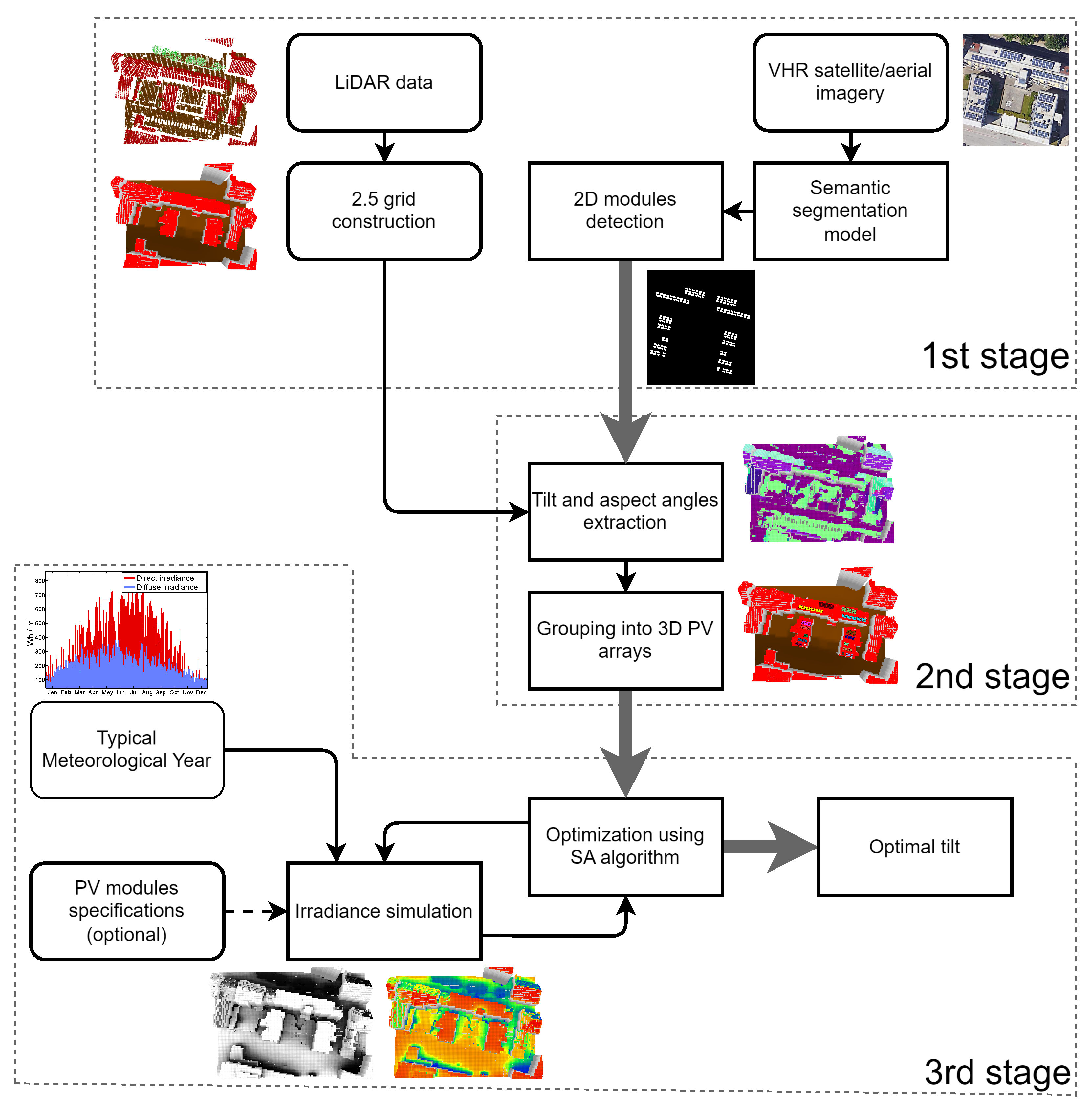
The overall workflow of the proposed method is illustrated in Figure 2. In the first stage, VHR imagery is utilized to detect individual 2D modules using a U-shaped semantic segmentation model, which returns a coarse result that is then further refined using the Fine Optimization Module (FOM). The 2D width and height of each module can be easily extracted from the resulting detection. This segmentation approach takes advantage of advanced convolutional layers and skip connections inherent in the U-shaped architecture to effectively handle variations in PV module appearance due to different illumination conditions, module types, and partial occlusions. The subsequent refinement through FOM further corrects inaccuracies, addressing issues such as merging modules in close proximity or splitting larger modules erroneously.

Figure 2.
Workflow of the proposed method for optimization of detected arrays’ tilt angle based on fusion of VHR imagery and airborne LiDAR data.
In the second stage, airborne LiDAR data are processed into a 2.5D topological grid. This aids in estimating the tilt and aspect angles of the detected modules, which can then be used together with width and height information extracted from VHR imagery, allowing for accurate 3D reconstruction and positioning within the grid. In addition, the grid provides a detailed representation of the surrounding environment. It is crucial to note that typical airborne LiDAR point cloud data lack sufficient density to detect the entire modules’ 2D or 3D structures, as typical airborne LiDAR scans contain 5 to 10 points per 1 m2 [3]. Thus, VHR imagery remains indispensable. It should be noted that merely three 3D points detected on a module, from LiDAR scanning, are adequate to determine its geometric plane, as well as tilt and aspect angles from the plane’s normal vector. The detected and reconstructed 3D modules are then grouped into their respective 3D arrays based on their proximity and characteristics by using a clustering algorithm. Since the clustering process incorporates both geometric attributes (i.e., slope and aspect angles) and spatial position, it ensures that the modules belonging to the same physical PV array are accurately grouped together.
In the last stage, the optimization process then iteratively conducts a simulation of hourly solar irradiance throughout the entire year (i.e., solar potential) for each module (within a given array) after the hypothetical tilt angle change in each optimization iteration. The irradiance simulation considers the additional input of the location’s Typical Meteorological Year (TMY) for the direct and diffuse irradiance data and optionally modules’ specifications if electricity production is to be estimated. Moreover, the irradiance simulation considers direct and anisotropic Perez diffuse irradiances, as well as shadowing in-between PV arrays and from surrounding surfaces (e.g., buildings, hills) represented in the 2.5D grid. The optimization result is an optimal tilt angle estimation for each PV array, in order to maximize annual solar irradiance for corresponding modules for the given array.
The next three subsections provide a more detailed description of the proposed method, covering the detection of 2D modules, their 3D reconstruction, and finally the optimization of their tilt angles.
2.1. Detection of 2D Modules in VHR Imagery
In the first stage, the detection of individual 2D modules is performed on the basis of VHR imagery. This can be accomplished using established semantic segmentation methods using U-shaped encoder–decoder architectures that have a good track record in VHR satellite imagery, namely, bidirectional aggregation network with occlusion handling (BAnet) [35], feature pyramid network based on attention aggregation (A2-FPN) [36], densely connected feature aggregation with Swin vision Transformer (DCSwin) [37], Multi-Attention Network (MANet) [38], and UNet-like Transformer (UnetFormer) [39]. The U-shaped architectures utilize several layers based on the encoding backbone to progressively encode the input image into high-dimensional feature space (i.e., feature embedding), effectively capturing complex features and patterns within the image. These high-dimensional features are then fed into decoding layers that reconstruct the target image (i.e., semantically annotated image). The semantic segmentation produces coarse binary classification, i.e., detection of individual modules (foreground) and disregarding the rest of the image (background). The coarse result is then further refined using FOM, similarly as recently performed by [21]. FOM is a simple U-shaped method over the coarse binary segmentation result, where, in the encoding phase, the feature embedding is achieved using 4 convolutional layers complemented with batch normalization and ReLU activation, while, in the decoding phase, the feature space is upsampled using 4 transposed convolutional layers. Each decoder stage also incorporates skip connections by concatenating the corresponding encoder output, allowing the preservation of high-frequency details. In the results, it is shown that the aforementioned methods are highly suitable for the detection of modules, by also trying various encoder backbones with additional ablation analysis of how FOM significantly affects the quality of the detection.
To the authors’ knowledge, only the ground truth data annotating the arrays or PV systems within VHR imagery is publicly available, since, at the time of writing of this paper, no datasets annotating individual modules in VHR imagery were found. Hence, in this paper, a basic image processing pipeline is introduced, which requires some manual postprocessing, designed to create ground truth data for individual modules in VHR imagery. These data can then be used for training the semantic segmentation models. Initially, the RGB color-coded image is converted to the YCbCr color space, and then only the luminance component (Y) is used for subsequent detection. This reduces the computational complexity from three channels (RGB) to a single channel, which sufficiently defines the shape and structure of the modules. Next, a morphological maxtree [40] is constructed through all gray levels to detect all connected components that approximate rectangles (Figure 3b). Hence, only quadrilaterals with the four inner angles within the range of are retained (Figure 3b). These are then further filtered based on their neighborhood, wherein each rectangle (a potential module) requires at least two neighboring rectangles with a similar 2D size (i.e., width and height) and spatial orientation (Figure 3c).
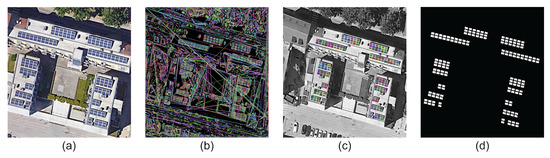
Figure 3.
Steps to create ground truth data for module detection: (a) input VHR image, (b) image preprocessing, (c) detection of contours, and (d) filtering and thresholding for creating module masks, which are further manually processed.
The retained rectangles are thresholded into a binary mask representing the modules’ ground truth data. Lastly, manual postprocessing is performed to remove potential outliers (incorrectly detected modules) or to add missing modules (Figure 3d), since this image processing pipeline cannot detect modules that are obstructed by the surrounding context. Traditional image processing methods are inherently limited by their reliance on predefined heuristics, making them susceptible to performance degradation when faced with complex scenarios common in aerial imagery. Specifically, these methods lack the capacity to integrate broader contextual information, such as varying lighting conditions, shadows, occlusions caused by nearby objects, or partial module visibility, all of which significantly affect PV module detection accuracy. Deep learning techniques, in contrast, leverage extensive contextual cues and spatial relationships within the data, thus providing superior adaptability and robustness for detecting PV modules even under challenging conditions, as will be shown in the results section of this paper. Moreover, the mask obtained in Figure 3d does not provide any instance-based detection of individual PV modules, and this has to be further performed, for example, with a region filling algorithm.
In order to have a more accurate estimation of module sizes, it is highly advised to use orthorectified and georeferenced VHR images (i.e., true orthophotos), wherein objects are viewed in a top–down orthographic projection. Most VHR imagery is already readily georeferenced, where, for each pixel, a precise geolocation is known. Since the airborne LiDAR point cloud is in many cases also already georeferenced, this allows precise spatial correspondence between VHR pixels with the LiDAR point cloud. In some cases, remote sensing data can be georeferenced with different geographic coordinate systems; hence, coordinate re-projection must be performed prior to ensure that all datasets have the same coordinate system. Producing a true orthophoto from VHR images is beyond the scope of this paper; however, there are several methods for this purpose, as detailed in [41,42]. It should also be noted that the ground truth data used for semantic segmentation models do not need to be orthorectified, which allows for potentially larger training datasets.
The width and height of each given module can then be estimated from the pixels of the modules detected in VHR. This provides important information in creating an accurate 3D reconstruction of the modules. To estimate the tilt and aspect angles, 3D information is necessary, which can be derived from airborne LiDAR data, as will be described in the next subsection.
2.2. Three-Dimensional Reconstruction of Detected Modules Using LiDAR Data
At first, the LiDAR point cloud data are classified into buildings, terrain, and vegetation, which can be performed by using any point cloud semantic segmentation model such as FKAConv [43] (see Figure 4a). This point cloud is then inserted into a 2.5D equidistant topological grid G with a predefined resolution of [m2]. This is vital since the point cloud does not inherently possess any topological information. The height and class of each individual cell is determined by the highest point located within a given cell , as follows:
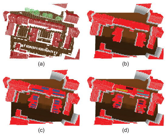
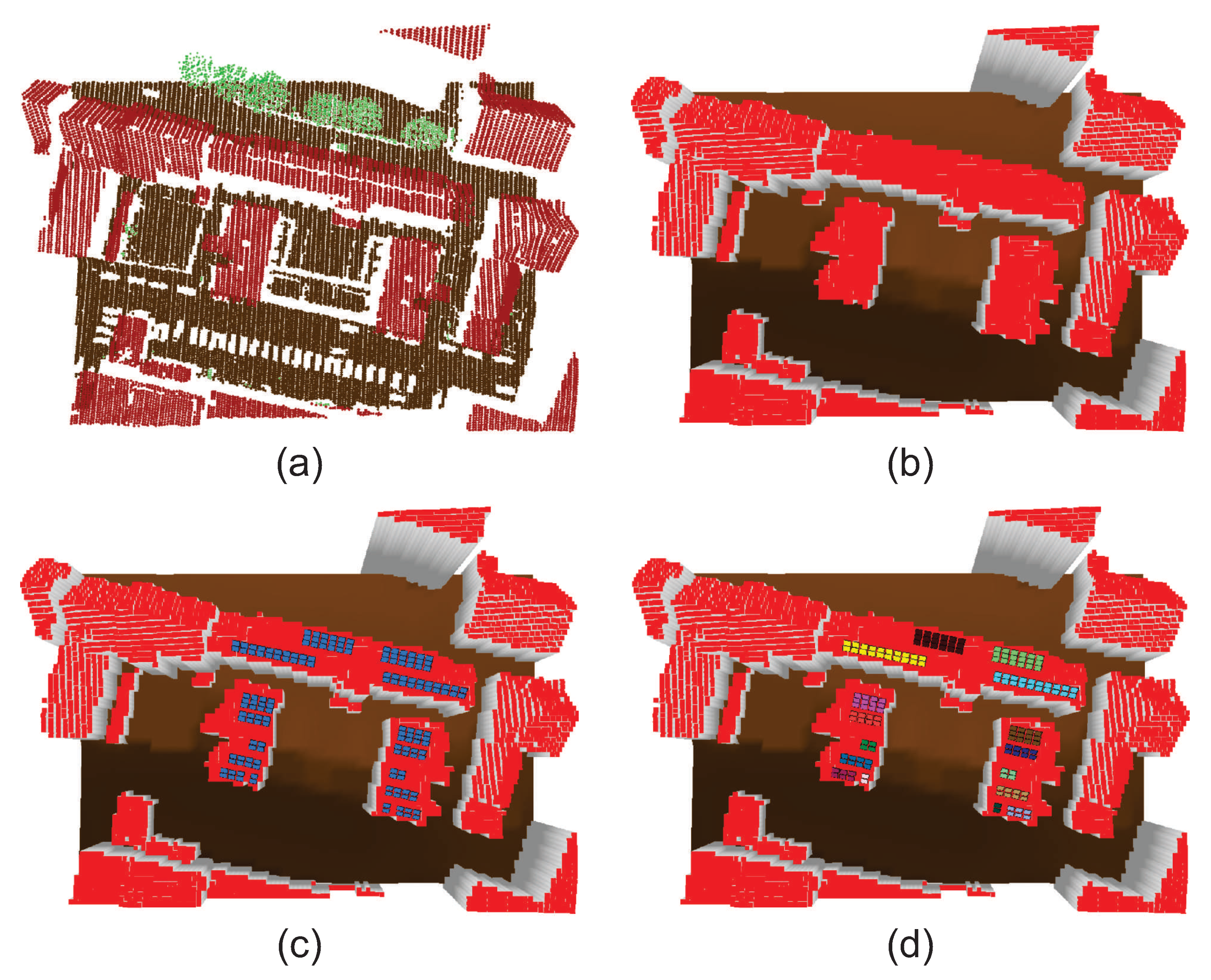
Figure 4.
Visualization of example 3D reconstruction and grouping of modules: (a) raw classified point cloud data into terrain, buildings, and vegetation; (b) constructed 2.5D grid; (c) reconstruction of 3D modules; (d) colored by DBSCAN-based grouping (i.e., for each array).
In case some cells are empty due to varying point cloud densities from artifacts such as multiple laser reflections, the cell’s values are filled with Inverse Distance Weighting (IDW) interpolation, as follows:
where is a set of neighboring cells of and . Consequently, the grid G resembles a digital surface model (DSM), but with the added distinction that the cells are classified (see Figure 4b). The normal vector of each cell is determined using the best-fit plane algorithm [44], considering the points P located within a given cell and its neighboring cells based on the 8-neighborhood. This is performed by minimizing the sum of squared distances from P to the plane, where a covariance matrix is constructed, as follows:
where is the centroid of P. After the eigendecomposition of , the eigenvector corresponding to the smallest eigenvalue of is the normal vector . The tilt (inclination) and aspect (orientation) angles of a given cell can then be estimated directly from as follows:
The grid retains the geographic coordinate system used by the georeferenced LiDAR point cloud. As a result, it can be seamlessly integrated with information about 2D modules detected in VHR imagery, provided that the VHR and LiDAR datasets share the same geographic coordinate system. The tilt (inclination) and aspect (orientation) angles for a given module are then estimated as follows:
where and belong to n cells spatially overlapping the given in the XY plane. Afterwards, these cells are decreased (i.e., flattened) by the modules’ vertical height, which is estimated as follows:
Next, a 3D polygon is generated for each module using given , , , and (see Figure 4c), where the given polygon’s relative vertices’ 3D position is defined as follows:
Finally, the modules are grouped on the basis of their proximity, as well as aspect and tilt angles, since it is computationally less expensive to optimize modules that belong to the same array. Another reason is that, in real PV installation scenarios, the modules are typically bundled into arrays, sharing the same installation platform beneath, where the tilt angle is set by the platform. For this purpose, the well-known DBSCAN clustering algorithm [45] is used, where each module is represented by its feature vector . Two given modules belong to the same cluster (i.e., array) if the following conditions are satisfied:
where d is a Euclidean distance function, j and k () define the indices of different modules, is the positional threshold, and is the feature vector threshold. The parameter in DBSCAN defines the minimum number of entities to form a cluster, which is set to 1. An example result of grouping of modules into arrays can be seen in Figure 4d. Each array has the following properties:
where N denotes the number of modules belonging to given .
2.3. Optimization of Tilt Angle Based on Irradiance Simulation
In the third stage, the tilt angle optimization is executed for each array. In this work, the well-known SA algorithm [46,47] is used due to its suitability for tackling nonlinear optimization of a single real-valued parameter. At first, the most optimal tilt angle is set to the existing configuration, i.e., , where b annotates the best solution. Then the algorithm iteratively adjusts the tilt angle as follows:
where is the current iteration, L is the maximum number of iterations’ input hyperparameter, q is the SA step size input hyperparameter, and is the current accepted solution of the tilt angle, which is initially equal to . Afterwards, the following is calculated for the given iteration l:
where S is a function for per-annum solar irradiance estimation for a given array configuration, which will be described in more detail in continuation. The input hyperparameter T defines the temperature of the SA algorithm, which is the likelihood that a worse solution is accepted than the current solution . m is the so-called Metropolis criterion [47], which allows the SA algorithm to escape local minima when T is sufficiently high. Within a given iteration l, if , then . Otherwise, there is a chance that the current solution changes to , if holds.
The core of the optimization criteria is the irradiance simulation for each , where the goal is to maximize the amount of solar irradiance received. In this paper, the solar irradiance simulation approach is based on the previous work of the authors [8,48], which was rigorously validated regarding the accuracy. This approach takes into account shadowing from the surroundings (represented in the 2.5D grid), self-shadowing between modules, and direct irradiance and anisotropic diffuse irradiance based on the well-known Perez model. The per-annum estimated solar irradiance with an hourly time-step (i.e., the solar potential) for a given is estimated as follows:
where D and P are discrete functions for estimating direct and diffuse irradiance for arbitrary surfaces at a given time instance t [49]. These functions depend on the input horizontal irradiance measurements of direct and diffuse irradiances, as well as the surface’s tilt (inclination) and aspect (orientation) angles. Both and are generally obtained from TMY with an hourly temporal resolution for a given location, constructed by the Sandia method [50] using long-term pyranometer-based measurements at the given location. is perturbed in D by estimating the angle of incidence and the solar zenith angle for the given surface, where an additional input is the Sun’s spherical position defined as (i.e., solar azimuth and altitude). The Sun’s position for the given location can be estimated with the SolPos algorithm [51]. To estimate diffuse irradiance, the Perez model is considered (for details, see [52]).
Finally, effects from shadowing have to be considered between the modules, as well as the surrounding environment. The shadowing for a given in instance t is estimated with a discrete function H. At first, for the given time-step t, the grid G is adjusted, where the cells’ heights are located within the 2D XY plane of a given . These cells can be found using the point-in-polygon algorithm. The height of such a cell is then estimated by bilinear interpolation of the 3D polygon’s four vertices for a given , as follows:
where and . Then, the shadowing for a given cell within that belongs to is estimated for time instance t, as follows [8]:
where is a grid cell belonging to , and is a cell along the path of the directional vector pointing to the relative position of the Sun (in Cartesian coordinates) for time instance t. The main reason shadowing is estimated using grid G is to decrease computational complexity, as this operation presents the bottleneck of solar irradiance simulation that is executed on the Graphics Processing Unit (GPU) (see [48]).
3. Results
To the authors’ knowledge, there is no publicly available VHR dataset annotating individual modules. Hence, initially, a training dataset was generated from publicly available VHR satellite imagery over Slovenia provided by Google (Airbus, CNES/Airbus, Maxar Technologies, 2024). This dataset comprises 105 satellite images with a resolution of 512 × 512 pixels, where modules were annotated utilizing the presented unsupervised method with manual corrections to obtain ground truth data. Moreover, the dataset underwent simple augmentations through 90°, 180°, and 270° rotations and horizontal and vertical flips, which enhanced the dataset size to 1260 images. Subsequently, the augmented dataset was split using a 4:1:1 rule into learning, validation, and testing sets.
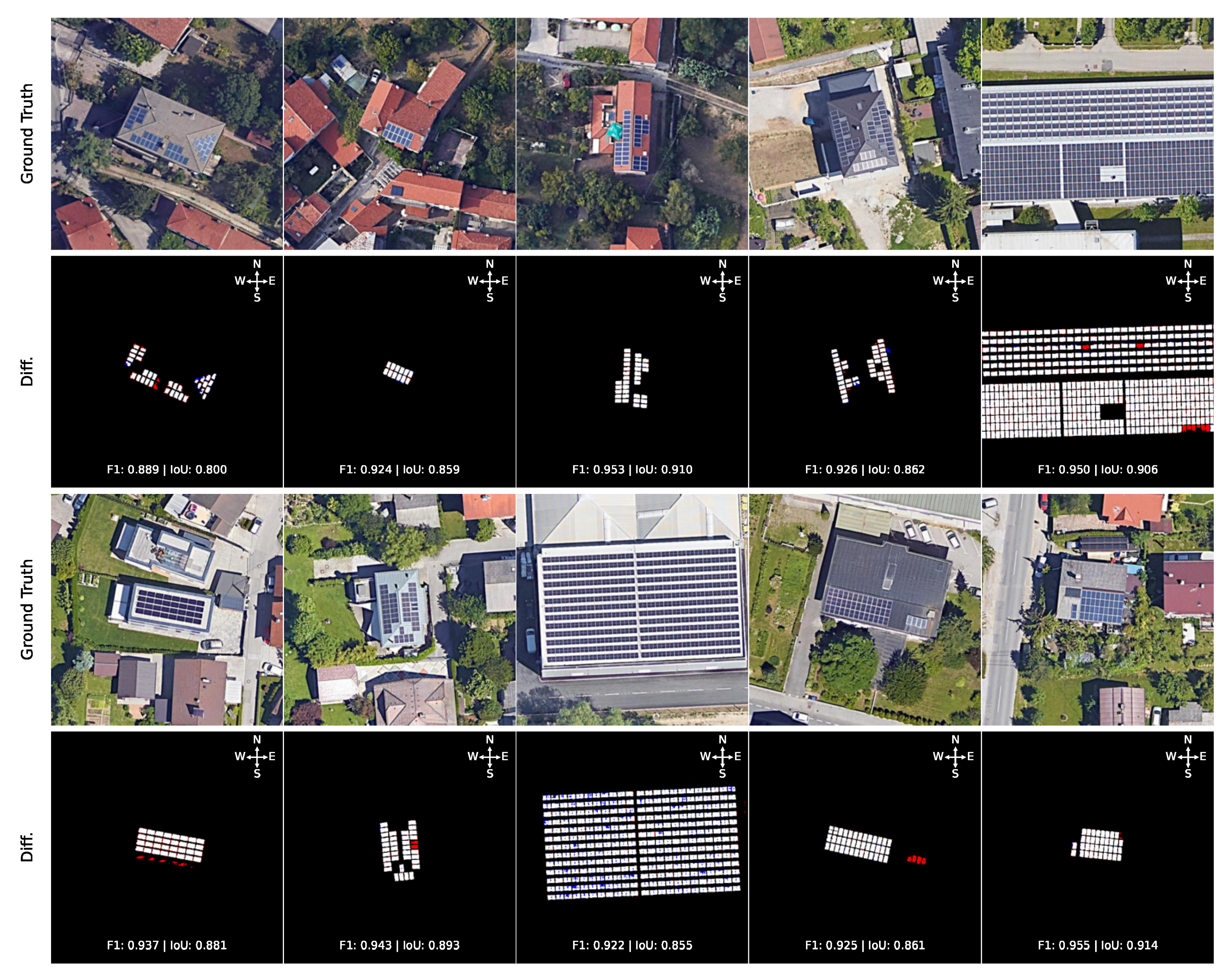
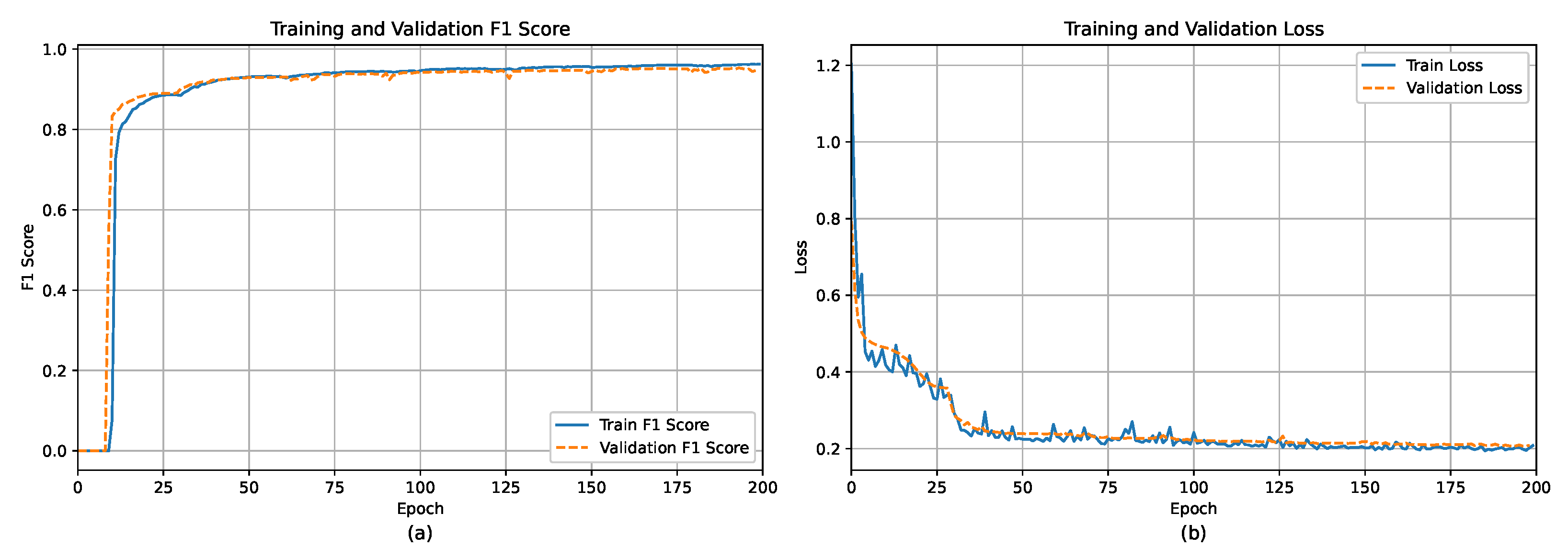
Various semantic segmentation methods were evaluated for the automatic detection of individual 2D modules using methods based on U-shaped deep learning architectures with different encoder backbones, as shown in Table 1. The encoder backbones’ weights were pretrained on ImageNet [53], where, for the encoder backbone, the traditional ResNet-18 encoder [54] was used. For newer methods [37,38,39], the Swin vision Transformer [55] was also considered, as well as EfficientNet-b5 and SE-ResNeXt50, which reported good results for the whole PV system/array detection in a recent work [25]. Table 1 also provides ablation analysis when using detection complemented with FOM and without, where the results were superior when FOM [21] was applied at the end. The choice of suitable hyperparameters was performed by using a grid search approach. Each model was trained for 200 epochs with early stop if no improvements were observed within 20 epochs, using the Adam optimizer with a weight decay of 0.00025, an initial learning rate of 0.001, and an adaptive learning rate scheduler using Cosine Annealing with warm restarts ( = 25 and = 0.00001). The loss function was set as the joint loss of SoftCrossEntropy and Dice loss functions [39]. The performance of each model was assessed using the average intersection-over-union (IoU) and the harmonic mean of precision and recall (F1). In addition, the computational complexity of each model was evaluated using GFLOPS metrics [G] and its size based on the number of parameters in millions [M]. Each model was run 5 times using 5-fold cross-validation in order to ensure higher robustness of the results. An example visual prediction error of module detection using the best model FT-UnetFormer (with SwinTransformer encoder backbone) based on a fully Transformer network is shown in Figure 5, where the model can overpredict in case of false positives like skylights or underpredict due to the non-homogeneous color of the modules. Furthermore, Figure 6 shows the training and validation F1 score and loss per epoch, respectively. The model can reach an above 0.8 F1 score after 15 epochs, which hits a granularity level of approximating an array, but not an individual module, for which more epochs of training were required.

Table 1.
Averaged inference results of various deep learning methods for individual 2D modules’ detection after 5-fold cross validation run on the test dataset. The highest result is styled in bold. Ablation analysis is shown when performing detection with or without FOM (Jianxun et al., 2023) [21].
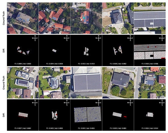
Figure 5.
Inference results on sample images from the testing dataset, where the 1st and 3rd rows show the original satellite imagery, while the 2nd and 4th rows show the difference between the ground truth masks of detected modules and the results of detection using an FT-UnetFormer model with corresponding IoU and F1 metrics per image. The red and blue colors indicate overprediction and underprediction, respectively.
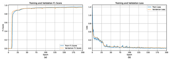
Figure 6.
Results of the FT-UnetFormer with SwinTransformer model regarding per-epoch change of (a) F1 score and (b) learning loss for training and validation data, respectively.
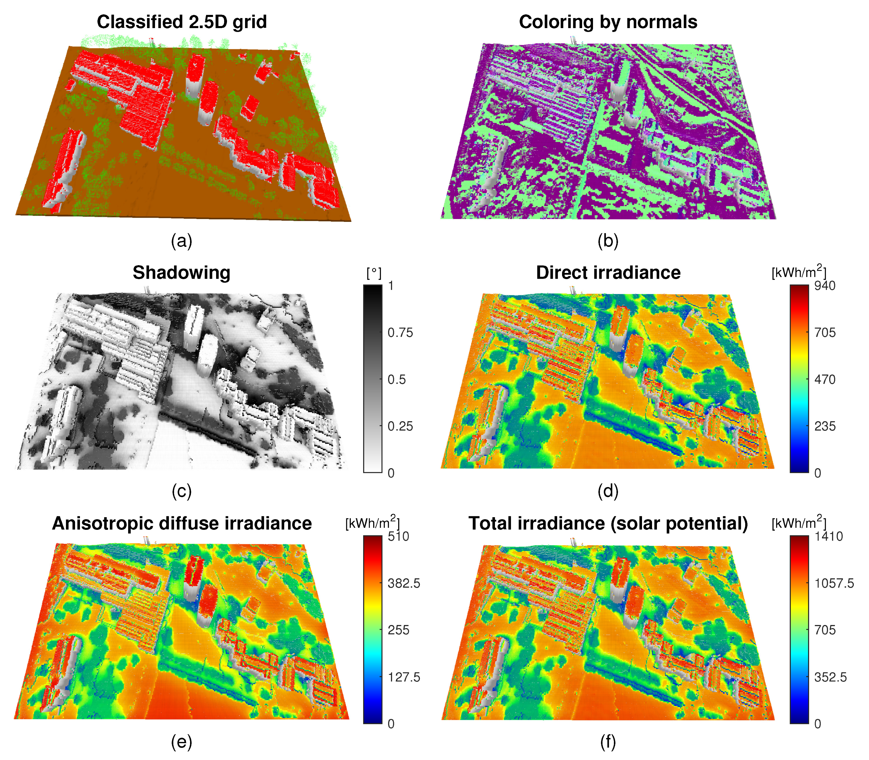
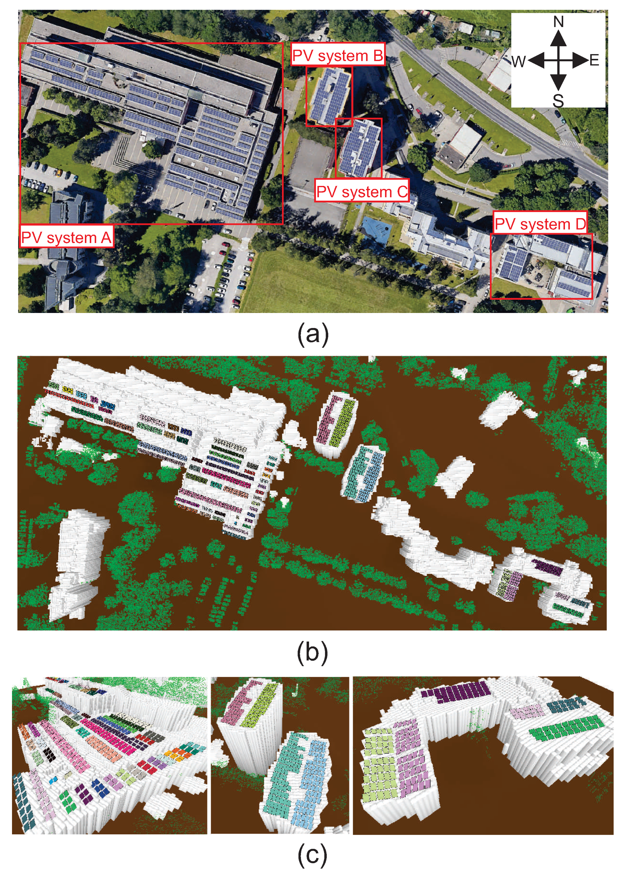
The validation of the proposed method was carried out on PV systems installed at the University of Maribor campus’s buildings in Slovenia, geolocated at 46° 33′ 48.77″ N, 15° 37′ 30.68″ E. Figure 7a shows a classified 2.5D grid from airborne LiDAR data for the given campus location with a resolution of , where the coloring is based on three classes of the underlying point cloud data, namely, buildings, terrain, and high vegetation. Figure 7b shows the coloring based on estimated normal vectors for each cell in the grid (used to derive slope and aspect angles), while Figure 7c–f show an example result of using the considered solar irradiance simulation method for different components, namely, average shadowing (Figure 7c), direct irradiance (Figure 7d), anisotropic diffuse irradiance (Figure 7e), and total solar irradiance—the solar potential (Figure 7f). By using the proposed method, this simulation is repeatedly re-run within the SA optimization algorithm in each iteration when the tilt angle is adjusted for each PVA. The LiDAR data, as well as long-term direct and diffuse horizontal meteorological measurements, in order to construct TMY, were provided by the Slovenian Environment Agency. The meteorological data were sourced from a national meteorological station located 5 km away at the Edvard Rusjan International Airport. Figure 8a shows the orthorectified satellite imagery along with the information from the corresponding PV systems, whereas Figure 8b,c visualize the reconstructed 3D modules from LiDAR and VHR data using FT-UnetFormer, colored by the array grouping. Details on the tilt and aspect angles extracted from the PV systems, as well as the dimensions of the modules, are provided in Table 2.
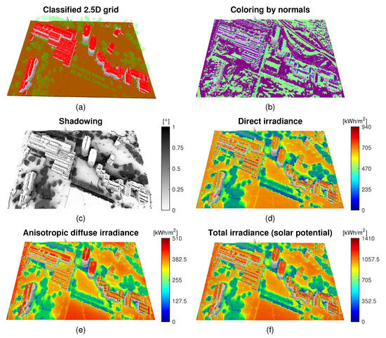
Figure 7.
Visualization of validation site in Maribor, Slovenia, where (a) is the constructed 2.5D classified grid from LiDAR data, (b) is the estimated normal vectors over the grid, (c) is the simulated average hourly shadowing per annum, and (d–f) present simulated average hourly direct, diffuse, and total irradiances per annum.
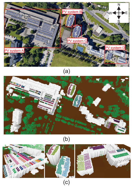
Figure 8.
Validation site in Maribor, Slovenia, where (a) is a satellite imagery of the site with annotations of the considered PV systems, (b) is reconstructed 3D arrays over 2.5D grid from airborne LiDAR and VHR data, and (c) is a zoom-in into the given PV systems.
Table 2.
Specifications of and angles of individual modules, as well as their sizes (i.e., ), number of arrays per system (i.e., ||), and installed capacity.
To validate the accuracy of the detected modules coupled with the solar irradiance simulation, additional specifications of the modules installed in all four photovoltaic systems were obtained. Each system utilizes Bisol BMU-215-2/233-type modules (233 Wp) with a nominal efficiency of 14.25% per square meter. The inverter model used is the Sunny Tripower STP 17000TL-10 [2]. The installed capacities of the PV systems A, B, C, and D are 228 kWp, 45 kWp, 45 kWp, and 49 kWp, respectively [2]. A comparison was made between the actual independent measurements (from 2018 to 2022 timespan) of electricity production from these PV systems and the estimated production derived from the irradiance simulation on the 3D reconstructed modules. To simulate electricity production, the estimated solar irradiance was multiplied by the nominal efficiency of each PV system (as detailed in Table 2). The simulated electrical energy production for each array was aggregated to the corresponding PV system. The estimation error was calculated using the Mean Absolute Percentage Error (MAPE) metric, and the comparative results are presented in Table 3.
Table 3.
Average electrical energy produced of the given PV systems in the timeline 2018–2022, with comparison between simulated expected energy production and the calculated error using MAPE metric. Further comparison is provided between simulated energy production using detected tilt angles and optimal tilt angles.
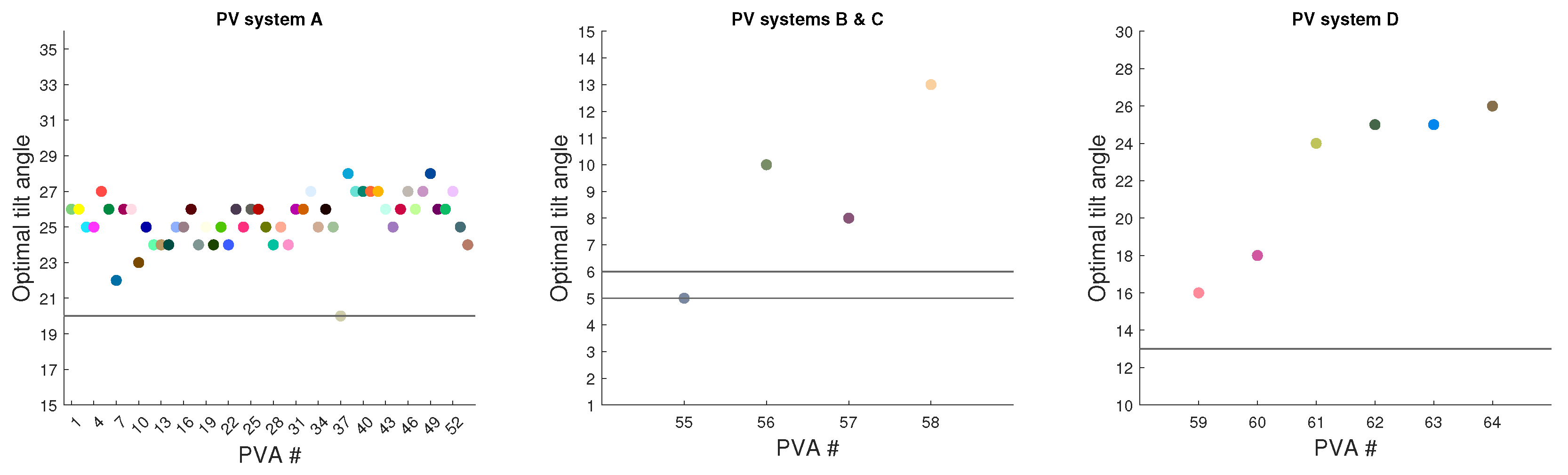
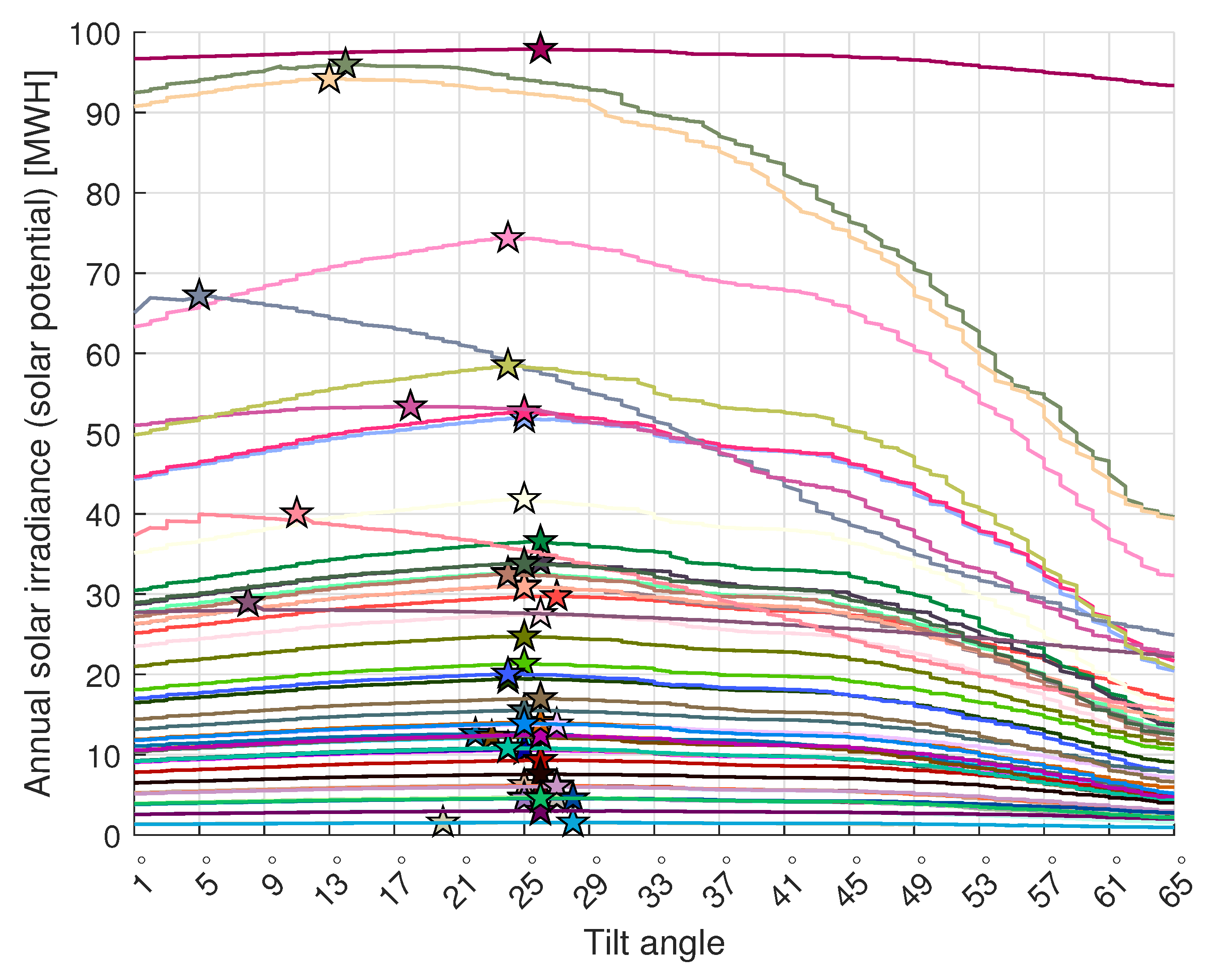
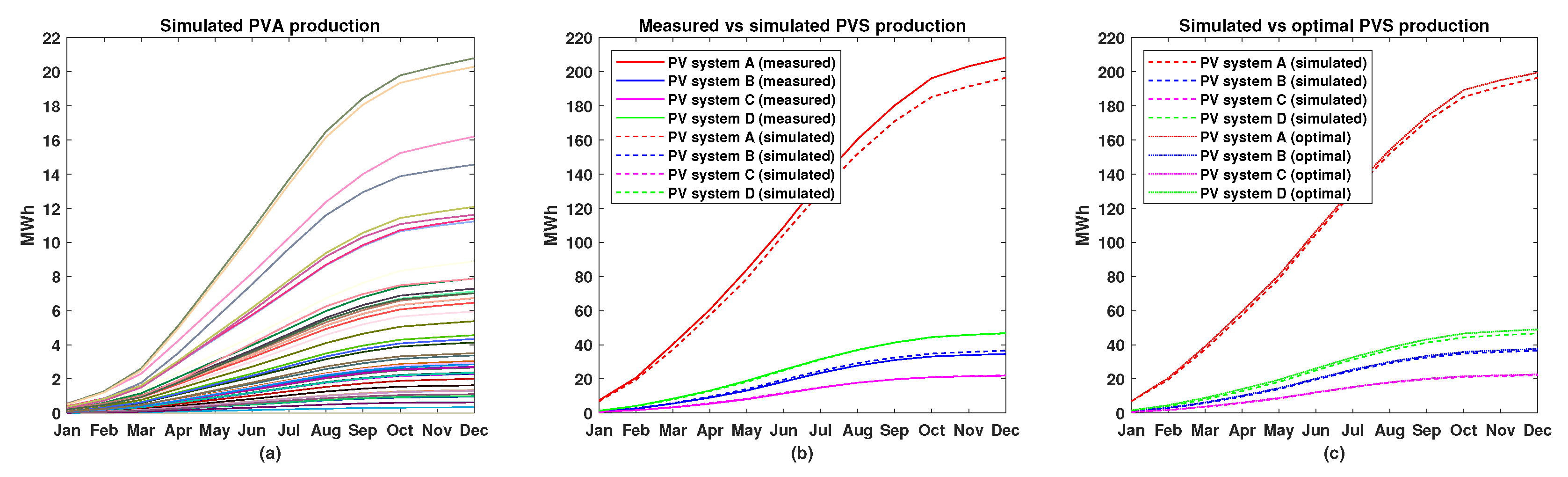
Finally, the arrays have been optimized to have an optimal tilt angle based on the proposed method of using the SA algorithm. Figure 9 shows a comparison of real tilt angles and optimally detected tilts for each array. Moreover, to verify that SA found the optima, the annual solar irradiance per array has been estimated using an exhaustive search by trying all physically viable tilt angles, as seen in Figure 10. The optimization results at the PV system level are shown in Table 3, where improvements from 1.5 % to 4.9 % were observed. This is not surprising, as the arrays installed at systems A and D had already tilt angles close to optimum based on the geographic latitude, while the spacing ensured minimum shadowing. On the other hand, the tilt angle could not be significantly changed for systems B and C, which were installed on slightly sloped rooftops, and the increase in tilt would increase the amount of shadowing between modules due to no spacing between modules. Further visualization of the results is shown in Figure 11, where cumulative electrical energy production for each PVA (Figure 11a) is shown, and a comparison between estimated cumulative production and measurements for each PV system is provided (see Figure 11b). Finally, a comparison between the estimated production using detected tilt angles and the optimal tilt angles for each PV system is shown in Figure 11c.
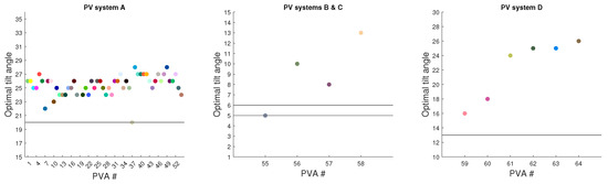
Figure 9.
Optimal tilt estimated with the proposed method for each array for all four PV systems. The black lines represent the real slopes used by the arrays within the given PV system. Colors of the arrays correspond to colors in Figure 8b.
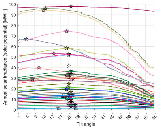
Figure 10.
Estimated total annual solar irradiance per detected array by changing the tilt angle with an exhaustive method. The stars denote the optimum tilt angles for a given PV array, where the received solar irradiance is maximized.
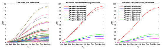
Figure 11.
(a) Simulated cumulative electrical energy production from individual arrays, where the colors correspond to colors in Figure 8b,c; (b) comparison between cumulative measured and simulated electrical energy production from the four PV systems; and (c) comparison between cumulative simulated and optimal electrical energy production from the four PV systems.
These results highlight the importance of considering site-specific factors for PV systems’ tilt angle optimization. Although some systems (A and D) were already close to optimal configuration, others (B and C) faced practical limitations that restricted their optimization potential. The results have demonstrated that even small improvements in arrays’ tilt angle can lead to measurable increases in energy production, especially during several years of operation. Furthermore, in many cases, adjustment of the tilt angles per array does not require significant on-site workload.
4. Discussion
4.1. Generalization to Large Scale
The proposed optimization method is highly generalizable to the regional or even global scale, provided that local input data are available, such as VHR aerial imagery, LiDAR data, and meteorological measurements. First, the detection of PV modules in VHR imagery does not differ fundamentally between different geographical regions, as most standard PV modules share highly similar visual characteristics, such as rectangular shape, homogeneous color, and regular grid patterns. Hence, a well-trained semantic segmentation model can be widely applicable, even in geographically diverse settings, as long as the underlying resolution and VHR image quality are sufficient. Second, although the proposed method was validated locally, due to the availability of detailed validation data, the solar irradiance and shadowing methodology considered within the optimization has already been validated by previous works by the authors on the installation of hypothetical new PV modules’ placement [8] or for large-scale applications [48]. In addition to the previous work of the authors, the approach considered for the estimation of direct irradiance and the effects of shading can be applicable to any geographical location with diverse climate conditions, as was shown by Duffie et al. [49]. Moreover, the Perez anisotropic irradiance model [52,56] used is a well-known approach to estimate diffuse irradiance for any geographical location.
Finally, the expected energy gains on regional or global scales could be significant even when the tilt angle is improved by 5 % for existing photovoltaic systems, especially when considering several years of future operation. Such a large-scale detailed analysis is beyond the scope of this paper and can be considered as an extension for future work, where HPC or cloud-based computing would be required.
4.2. Computational Cost
Although the considered semantic segmentation models for module detection require training in representative datasets, transfer learning techniques could be used to reduce training times. However, once the chosen model has been fully trained, the time required to perform inference to detect PV modules on new VHR images is not an intensive task. On the other hand, the proposed SA-based optimization of the tilt angle can be computationally demanding due to multiple iterations in the estimation of solar irradiance for each PV array. However, the irradiance estimation approach considered by the authors can be parallelized efficiently using GPUs, as the authors showed in [48], which can substantially reduce computational burden, especially when estimating shadowing effects. Furthermore, for a larger-scale deployment, the proposed methodology could be run within high-performance computing (HPC) environments, or distributed cloud platforms could be employed to handle more computationally demanding tasks. Finally, the proposed method does not require real-time deployment, as such optimization should be run only once for a given PV system, unless the effects from environmental obstructions change in the near future (e.g., new high-rise buildings or taller vegetation) or new PV systems are installed.
4.3. Data Limitations
The presented method also has limitations with respect to the input data, as it is highly dependent on the resolution of the VHR image data and the density of the LiDAR point cloud. If the resolution of the VHR image is too small, the individual modules cannot be effectively detected, while a low LiDAR point cloud density would yield an insufficient number of points to detect the tilt and aspect angles accurately. Moreover, the proposed method requires orthorectified VHR image data, which might not always be available, as well as georeferencing of VHR and LiDAR in the same geographic coordinate system. Although VHR imagery is now accessible for most urban and suburban areas through various commercial providers (e.g., Maxar, Airbus), licensing and data costs may vary by region. For regions lacking extensive LiDAR scans, alternative 3D acquisition methods may be used, such as photogrammetry, structure from motion from UAVs [29], or publicly available coarse-resolution digital surface models (e.g., derived from multiview satellite imagery). Although these alternatives often have lower spatial resolution compared with airborne LiDAR, they can still be utilized to obtain approximate surface geometric details, which are sufficient in many practical use cases of solar energy estimations such as that considered in this work. It is also reasonable to expect that the amount of publicly available georeferenced VHR and LiDAR data will increase substantially over the next decade; hence, this will provide better opportunities to utilize such a method on a larger scale.
From a solar energy modeling perspective, region-specific meteorological data, especially horizontal global and diffuse irradiance measurements from pyranometer devices, remain central. In regions where there are no high-frequency local measurements, reanalysis datasets or satellite-based global products (e.g., NASA POWER use [57]) can provide the necessary direct and diffuse irradiance input to construct TMY for a given region.
4.4. Real-World Constraints
Even when all required input data are available and the proposed method achieves high accuracy in the detection of PV arrays and their tilt angle optimization, certain practical considerations may limit its direct applicability. The method assumes that the tilt angle of each PV array can be feasibly adjusted; in reality, mechanical or structural constraints can prevent physical alterations. However, a physical change in the tilt angle can be made if a renovation or longer maintenance is performed on the given PV system, where the expected physical workload cost should be lower than the expected long-term energy production gains from the tilt angle adjustment. Finally, while the method can estimate optimal tilt angles from a purely technical point of view, real-world installations must also account for the broader structural and possible regional regulatory conditions governing the design and maintenance of the PV systems.
5. Conclusions
In this paper, a novel method was introduced for detecting individual photovoltaic (PV) modules by fusing remote sensing data from airborne Light Detection and Ranging (LiDAR) point cloud and Very High Resolution (VHR) satellite imagery. Before the proposed method was tested, several various semantic segmentation methods based on U-shaped architectures were trained on a newly annotated VHR dataset for the detection of 2D modules. The fully Transformer-based method FT-UnetFormer with the SwinTransformer encoder backbone provided the highest results in terms of IoU and F1 metrics, with the Fine Optimization Module (FOM) applied, yielding superior results. The proposed method was then tested on an airborne LiDAR scan and VHR imagery of the University of Maribor campus. The detected 2D modules were successfully reconstructed in 3D and grouped into 3D arrays. A state-of-the-art solar irradiance simulation method was considered, accounting for shadowing from the surroundings and anisotropic diffuse irradiance, in order to estimate the total per-annum received solar irradiance of each module and, consequently, the expected electricity production using the nominal efficiency of a given module. The simulated electricity production closely matched the electricity measurements of four PV systems at the campus, with an error of below 6.7 %. Finally, the proposed optimization using Simulated Annealing (SA) was used to estimate the potential increase in production if the tilt angle changed, where an increase of up to 4.9 % was estimated in the best case scenario.
This research also marks the first effort to demonstrate that the fusion of remote sensing data, coupled with a deep learning model, solar irradiance simulation, and optimization, can estimate the optimal tilt angles for existing array installations automatically, which has not been performed before. Therefore, the authors anticipate that the proposed method is highly useful in dense urban environments with a high concentration of obstructions, where the optimization of tilt angles is more crucial due to increased shadowing. Moreover, the proposed method could be seamlessly integrated with standard PV monitoring infrastructures (e.g., SCADA [58] or other smart metering platforms) that track real-time power output, meteorological conditions, and fault status. By accessing these data streams, the method performance assessments could be calibrated or validated against on-site measurements, thus enhancing accuracy and reliability for tilt angle optimization. In turn, continuous monitoring could enable a feedback loop, ensuring that any tilt angle modifications translate into measurable gains.
For future work, developing more advanced semantic segmentation models tailored for the detection of PV modules could yield improved accuracy, especially in challenging urban environments characterized by strong shadows, oblique viewing angles, or partial occlusions. Additionally, the proposed method could be extended to consider finding the optimal aspect angle for a given PV array, under the constraints that rotation would be physically possible in case of obstructions or available surface area. Furthermore, migrating from a 2.5D topological grid to full 3D triangulated models of buildings could offer more precise solar irradiance and shadowing analyses. Moreover, extending the irradiance simulation to account for thermal, wind-load and structural constraints would bring the optimization closer to real-world conditions. Further refinements could involve embedding cost–benefit calculations, e.g., considering local feed-in tariffs, within the optimization loop. Even in the case that the method provides marginal improvements, a small enhancement can be significant for large-scale PV systems over an extended operational period. Hence, distributed computing environments such as high-performance computing (HPC) platforms could boost computational efficiency for large-scale deployments, while periodic re-optimization incorporating new or updated geospatial data would enable periodic updating of optimization estimates as urban environments evolve over time. Therefore, the presented method will be highly useful for solar energy practitioners in the era of rapid urbanization and proliferation of solar energy, aiding in the mitigation of anthropocentric climate change and enabling a more sustainable living.
Author Contributions
Conceptualization, N.L.; methodology, N.L.; software, N.L.; validation, N.L. and M.B.; investigation, S.S. and K.S.; data curation, S.S. and K.S.; writing—original draft, N.L.; writing—review and editing, S.S., K.S., G.Š., D.M., B.Ž. and M.B.; visualization, N.L.; supervision, G.Š., D.M. and B.Ž.; funding acquisition, N.L. and D.M. All authors have read and agreed to the published version of the manuscript.
Funding
The authors acknowledge financial support from the Slovenian Research and Innovation Agency (Research Project No. J7-50095 and Research Core Funding Nos. P2-0041 and P2-0115).
Institutional Review Board Statement
Not applicable.
Informed Consent Statement
Not applicable.
Data Availability Statement
The input VHR data used are publicly available through the Google Maps service (data providers Google, Airbus, CNES/Airbus, Maxar Technologies 2024) and the open LiDAR data of Slovenia through the Slovenian Environmental Agency LIDAR portal (https://gis.arso.gov.si/evode/profile.aspx?id=atlas_voda_Lidar@Arso, accessed: 1 June 2024). The agency also provides long-term global and diffuse irradiance measurements for Slovenia, available at its open web archive (https://meteo.arso.gov.si/met/sl/archive/, accessed: 5 June 2024). The created georeferenced ground truth dataset with annotated module masks and the trained deep learning models will be available on request.
Acknowledgments
The authors thank the VHR imagery data providers Google, Airbus, CNES/Airbus, and Maxar Technologies 2024 and the Slovenian Environmental Agency for providing the long-term irradiance measurements and classified LiDAR data.
Conflicts of Interest
The authors declare that they have no conflicts of interest.
References
- Gassar, A.A.A.; Cha, S.H. Review of geographic information systems-based rooftop solar photovoltaic potential estimation approaches at urban scales. Appl. Energy 2021, 291, 116817. [Google Scholar] [CrossRef]
- Seme, S.; Lukač, N.; Štumberger, B.; Hadžiselimović, M. Power quality experimental analysis of grid-connected photovoltaic systems in urban distribution networks. Energy 2017, 139, 1261–1266. [Google Scholar] [CrossRef]
- Petrie, G.; Toth, C.K. Airborne and spaceborne laser profilers and scanners. In Topographic Laser Ranging and Scanning; CRC Press: Boca Raton, FL, USA, 2018; pp. 89–157. [Google Scholar] [CrossRef]
- Sredenšek, K.; Štumberger, B.; Hadžiselimović, M.; Mavsar, P.; Seme, S. Physical, geographical, technical, and economic potential for the optimal configuration of photovoltaic systems using a digital surface model and optimization method. Energy 2022, 242, 122971. [Google Scholar] [CrossRef]
- Özdemir, S.; Yavuzdoğan, A.; Bilgilioğlu, B.B.; Akbulut, Z. SPAN: An open-source plugin for photovoltaic potential estimation of individual roof segments using point cloud data. Renew. Energy 2023, 216, 119022. [Google Scholar] [CrossRef]
- Aslani, M.; Seipel, S. Automatic identification of utilizable rooftop areas in digital surface models for photovoltaics potential assessment. Appl. Energy 2022, 306, 118033. [Google Scholar] [CrossRef]
- Žalik, M.; Mongus, D.; Lukač, N. High-resolution spatiotemporal assessment of solar potential from remote sensing data using deep learning. Renew. Energy 2024, 222, 119868. [Google Scholar] [CrossRef]
- Lukač, N.; Špelič, D.; Štumberger, G.; Žalik, B. Optimisation for large-scale photovoltaic arrays’ placement based on Light Detection And Ranging data. Appl. Energy 2020, 263, 114592. [Google Scholar] [CrossRef]
- Aslani, M.; Seipel, S. Rooftop segmentation and optimization of photovoltaic panel layouts in digital surface models. Comput. Environ. Urban Syst. 2023, 105, 102026. [Google Scholar] [CrossRef]
- Kasmi, G.; Saint-Drenan, Y.M.; Trebosc, D.; Jolivet, R.; Leloux, J.; Sarr, B.; Dubus, L. A crowdsourced dataset of aerial images with annotated solar photovoltaic arrays and installation metadata. Sci. Data 2023, 10, 59. [Google Scholar]
- Arnaudo, E.; Blanco, G.; Monti, A.; Bianco, G.; Monaco, C.; Pasquali, P.; Dominici, F. A Comparative Evaluation of Deep Learning Techniques for Photovoltaic Panel Detection from Aerial Images. IEEE Access 2023, 11, 47579–47594. [Google Scholar] [CrossRef]
- Li, Q.; Krapf, S.; Shi, Y.; Zhu, X.X. SolarNet: A convolutional neural network-based framework for rooftop solar potential estimation from aerial imagery. Int. J. Appl. Earth Obs. Geoinf. 2023, 116, 103098. [Google Scholar] [CrossRef]
- Chen, Z.; Kang, Y.; Sun, Z.; Wu, F.; Zhang, Q. Extraction of Photovoltaic Plants Using Machine Learning Methods: A Case Study of the Pilot Energy City of Golmud, China. Remote Sens. 2022, 14, 2697. [Google Scholar] [CrossRef]
- Li, P.; Zhang, H.; Guo, Z.; Lyu, S.; Chen, J.; Li, W.; Song, X.; Shibasaki, R.; Yan, J. Understanding rooftop PV panel semantic segmentation of satellite and aerial images for better using machine learning. Adv. Appl. Energy 2021, 4, 100057. [Google Scholar]
- Ronneberger, O.; Fischer, P.; Brox, T. U-net: Convolutional networks for biomedical image segmentation. In Proceedings of the Medical Image Computing and Computer-Assisted Intervention–MICCAI 2015: 18th International Conference, Proceedings, Part III 18. Munich, Germany, 5–9 October 2015; Springer: Berlin/Heidelberg, Germany, 2015; pp. 234–241. [Google Scholar] [CrossRef]
- Wu, A.N.; Biljecki, F. Roofpedia: Automatic mapping of green and solar roofs for an open roofscape registry and evaluation of urban sustainability. Landsc. Urban Plan. 2021, 214, 104167. [Google Scholar] [CrossRef]
- Zhuang, L.; Zhang, Z.; Wang, L. The automatic segmentation of residential solar panels based on satellite images: A cross learning driven U-Net method. Appl. Soft Comput. 2020, 92, 106283. [Google Scholar] [CrossRef]
- Kausika, B.B.; Nijmeijer, D.; Reimerink, I.; Brouwer, P.; Liem, V. GeoAI for detection of solar photovoltaic installations in the Netherlands. Energy AI 2021, 6, 100111. [Google Scholar] [CrossRef]
- Zhang, J.; Jia, X.; Hu, J. SP-RAN: Self-paced residual aggregated network for solar panel mapping in weakly labeled aerial images. IEEE Trans. Geosci. Remote Sens. 2021, 60, 5612715. [Google Scholar] [CrossRef]
- Zhu, R.; Guo, D.; Wong, M.S.; Qian, Z.; Chen, M.; Yang, B.; Chen, B.; Zhang, H.; You, L.; Heo, J.; et al. Deep solar PV refiner: A detail-oriented deep learning network for refined segmentation of photovoltaic areas from satellite imagery. Int. J. Appl. Earth Obs. Geoinf. 2023, 116, 103134. [Google Scholar] [CrossRef]
- Jianxun, W.; Xin, C.; Weicheng, J.; Li, H.; Junyi, L.; Haigang, S. PVNet: A novel semantic segmentation model for extracting high-quality photovoltaic panels in large-scale systems from high-resolution remote sensing imagery. Int. J. Appl. Earth Obs. Geoinf. 2023, 119, 103309. [Google Scholar] [CrossRef]
- Tan, M.; Le, Q.V. EfficientNet: Rethinking Model Scaling for Convolutional Neural Networks. arXiv 2020. [Google Scholar] [CrossRef]
- Hu, J.; Shen, L.; Albanie, S.; Sun, G.; Wu, E. Squeeze-and-Excitation Networks. arXiv 2019, arXiv.1709.01507. [Google Scholar] [CrossRef]
- Szegedy, C.; Ioffe, S.; Vanhoucke, V.; Alemi, A. Inception-v4, inception-resnet and the impact of residual connections on learning. In Proceedings of the AAAI Conference on Artificial Intelligence, San Francisco, CA, USA, 4–9 February 2017; Volume 31. [Google Scholar] [CrossRef]
- Manso-Callejo, M.Á.; Cira, C.I.; Arranz-Justel, J.J.; Sinde-González, I.; Sălăgean, T. Assessment of the large-scale extraction of photovoltaic (PV) panels with a workflow based on artificial neural networks and algorithmic postprocessing of vectorization results. Int. J. Appl. Earth Obs. Geoinf. 2023, 125, 103563. [Google Scholar] [CrossRef]
- Guo, Z.; Lu, J.; Chen, Q.; Liu, Z.; Song, C.; Tan, H.; Zhang, H.; Yan, J. TransPV: Refining photovoltaic panel detection accuracy through a vision transformer-based deep learning model. Appl. Energy 2024, 355, 122282. [Google Scholar] [CrossRef]
- Wang, M.; Cui, Q.; Sun, Y.; Wang, Q. Photovoltaic panel extraction from very high-resolution aerial imagery using region—Line primitive association analysis and template matching. ISPRS J. Photogramm. Remote Sens. 2018, 141, 100–111. [Google Scholar] [CrossRef]
- Ji, C.; Bachmann, M.; Esch, T.; Feilhauer, H.; Heiden, U.; Heldens, W.; Hueni, A.; Lakes, T.; Metz-Marconcini, A.; Schroedter-Homscheidt, M.; et al. Solar photovoltaic module detection using laboratory and airborne imaging spectroscopy data. Remote Sens. Environ. 2021, 266, 112692. [Google Scholar] [CrossRef] [PubMed]
- Zefri, Y.; Sebari, I.; Hajji, H.; Aniba, G. Developing a deep learning-based layer-3 solution for thermal infrared large-scale photovoltaic module inspection from orthorectified big UAV imagery data. Int. J. Appl. Earth Obs. Geoinf. 2022, 106, 102652. [Google Scholar] [CrossRef]
- Mao, H.; Chen, X.; Luo, Y.; Deng, J.; Tian, Z.; Yu, J.; Xiao, Y.; Fan, J. Advances and prospects on estimating solar photovoltaic installation capacity and potential based on satellite and aerial images. Renew. Sustain. Energy Rev. 2023, 179, 113276. [Google Scholar] [CrossRef]
- Mayer, K.; Rausch, B.; Arlt, M.L.; Gust, G.; Wang, Z.; Neumann, D.; Rajagopal, R. 3D-PV-Locator: Large-scale detection of rooftop-mounted photovoltaic systems in 3D. Appl. Energy 2022, 310, 118469. [Google Scholar] [CrossRef]
- Chen, L.C.; Zhu, Y.; Papandreou, G.; Schroff, F.; Adam, H. Encoder-decoder with atrous separable convolution for semantic image segmentation. In Proceedings of the European Conference on Computer Vision (ECCV), Munich, Germany, 8–14 September 2018; pp. 801–818. [Google Scholar]
- Ravishankar, R.; AlMahmoud, E.; Habib, A.; de Weck, O.L. Capacity Estimation of Solar Farms Using Deep Learning on High-Resolution Satellite Imagery. Remote Sens. 2022, 15, 210. [Google Scholar] [CrossRef]
- Jurakuziev, D.; Jumaboev, S.; Lee, M. A framework to estimate generating capacities of PV systems using satellite imagery segmentation. Eng. Appl. Artif. Intell. 2023, 123, 106186. [Google Scholar] [CrossRef]
- Chen, Y.; Lin, G.; Li, S.; Bourahla, O.; Wu, Y.; Wang, F.; Feng, J.; Xu, M.; Li, X. Banet: Bidirectional aggregation network with occlusion handling for panoptic segmentation. In Proceedings of the IEEE/CVF Conference on Computer vision And Pattern Recognition, Seattle, WA, USA, 13–19 June 2020; pp. 3793–3802. [Google Scholar]
- Hu, M.; Li, Y.; Fang, L.; Wang, S. A2-FPN: Attention aggregation based feature pyramid network for instance segmentation. In Proceedings of the IEEE/CVF Conference on Computer Vision and Pattern Recognition, Nashville, TN, USA, 20–25 June 2021; pp. 15343–15352. [Google Scholar]
- Wang, L.; Li, R.; Duan, C.; Zhang, C.; Meng, X.; Fang, S. A novel transformer based semantic segmentation scheme for fine-resolution remote sensing images. IEEE Geosci. Remote Sens. Lett. 2022, 19, 6506105. [Google Scholar] [CrossRef]
- Chen, B.; Xia, M.; Qian, M.; Huang, J. MANet: A multi-level aggregation network for semantic segmentation of high-resolution remote sensing images. Int. J. Remote Sens. 2022, 43, 5874–5894. [Google Scholar] [CrossRef]
- Wang, L.; Li, R.; Zhang, C.; Fang, S.; Duan, C.; Meng, X.; Atkinson, P.M. UNetFormer: A UNet-like transformer for efficient semantic segmentation of remote sensing urban scene imagery. ISPRS J. Photogramm. Remote Sens. 2022, 190, 196–214. [Google Scholar] [CrossRef]
- Najman, L.; Couprie, M. Building the component tree in quasi-linear time. IEEE Trans. Image Process. 2006, 15, 3531–3539. [Google Scholar] [CrossRef]
- Gharibi, H.; Habib, A. True orthophoto generation from aerial frame images and LiDAR data: An update. Remote Sens. 2018, 10, 581. [Google Scholar] [CrossRef]
- Kavran, D.; Mongus, D.; Lukač, N. Buildings, Approximate True Orthophoto Construction From Satellite Imagery Using Semantic Segmentation and the ICP Algorithm. In Proceedings of the 2024 International Conference on Computer, Information and Telecommunication Systems (CITS), Girona, Spain, 17–19 July 2024; pp. 1–7. [Google Scholar] [CrossRef]
- Boulch, A.; Puy, G.; Marlet, R. FKAConv: Feature-kernel alignment for point cloud convolution. In Proceedings of the Asian Conference on Computer Vision, Kyoto, Japan, 30 November–4 December 2020. [Google Scholar]
- Fernández, O. Obtaining a best fitting plane through 3D georeferenced data. J. Struct. Geol. 2005, 27, 855–858. [Google Scholar] [CrossRef]
- Schubert, E.; Sander, J.; Ester, M.; Kriegel, H.P.; Xu, X. DBSCAN revisited, revisited: Why and how you should (still) use DBSCAN. ACM Trans. Database Syst. (TODS) 2017, 42, 1–21. [Google Scholar] [CrossRef]
- Bertsimas, D.; Tsitsiklis, J. Simulated annealing. Stat. Sci. 1993, 8, 10–15. [Google Scholar]
- Delahaye, D.; Chaimatanan, S.; Mongeau, M. Simulated annealing: From basics to applications. In Handbook of Metaheuristics; Springer: Berlin/Heidelberg, Germany, 2019; pp. 1–35. [Google Scholar] [CrossRef]
- Lukač, N.; Mongus, D.; Žalik, B.; Štumberger, G.; Bizjak, M. Novel GPU-accelerated high-resolution solar potential estimation in urban areas by using a modified diffuse irradiance model. Appl. Energy 2024, 353, 122129. [Google Scholar] [CrossRef]
- Duffie, J.A.; Beckman, W.A.; Blair, N. Solar Engineering of Thermal Processes, Photovoltaics and Wind; John Wiley & Sons, Inc.: Hoboken, NJ, USA, 2020. [Google Scholar] [CrossRef]
- Hall, I.; Prairie, R.; Anderson, H.; Boes, E. Generation of a Typical Meteorological Year; Technical Report; Sandia Labs.: Albuquerque, NM, USA, 1978. [Google Scholar]
- Reda, I.; Andreas, A. Solar position algorithm for solar radiation applications. Sol. Energy 2004, 76, 577–589. [Google Scholar] [CrossRef]
- Perez, R.; Ineichen, P.; Seals, R.; Michalsky, J.; Stewart, R. Modeling daylight availability and irradiance components from direct and global irradiance. Solar Energy 1990, 44, 271–289. [Google Scholar] [CrossRef]
- Deng, J.; Dong, W.; Socher, R.; Li, L.J.; Li, K.; Fei-Fei, L. Imagenet: A large-scale hierarchical image database. In Proceedings of the 2009 IEEE conference on computer vision and pattern recognition, Miami, FL, USA, 20–25 June 2009; pp. 248–255. [Google Scholar]
- He, K.; Zhang, X.; Ren, S.; Sun, J. Deep Residual Learning for Image Recognition. arXiv 2015, arXiv.1512.03385. [Google Scholar] [CrossRef]
- Liu, Z.; Lin, Y.; Cao, Y.; Hu, H.; Wei, Y.; Zhang, Z.; Lin, S.; Guo, B. Swin transformer: Hierarchical vision transformer using shifted windows. In Proceedings of the IEEE/CVF International Conference on Computer Vision, Montreal, BC, Canada, 11–17 October 2021; pp. 10012–10022. [Google Scholar]
- Perez, R.; Seals, R.; Ineichen, P.; Stewart, R.; Menicucci, D. A new simplified version of the Perez diffuse irradiance model for tilted surfaces. Sol. Energy 1987, 39, 221–231. [Google Scholar] [CrossRef]
- Sparks, A.H. nasapower: A NASA POWER global meteorology, surface solar energy and climatology data client for R. J. Open Source Softw. 2018, 3, 1035. [Google Scholar]
- Aghenta, L.O.; Iqbal, M.T. Development of an IoT based open source SCADA system for PV system monitoring. In Proceedings of the 2019 IEEE Canadian Conference of Electrical and Computer Engineering (CCECE), Edmonton, AB, Canada, 5–8 May 2019; pp. 1–4. [Google Scholar]
Disclaimer/Publisher’s Note: The statements, opinions and data contained in all publications are solely those of the individual author(s) and contributor(s) and not of MDPI and/or the editor(s). MDPI and/or the editor(s) disclaim responsibility for any injury to people or property resulting from any ideas, methods, instructions or products referred to in the content. |
© 2025 by the authors. Licensee MDPI, Basel, Switzerland. This article is an open access article distributed under the terms and conditions of the Creative Commons Attribution (CC BY) license (https://creativecommons.org/licenses/by/4.0/).