Abstract
Predicting innovation outcomes at the firm level continues to be an important but challenging goal for researchers and practitioners alike. In this study, multiple machine learning models, encompassing both ensemble-based and single-model approaches, were applied to data from the Community Innovation Survey. Methods included random forests, gradient boosting frameworks, support vector machines, neural networks, and logistic regression, each with hyperparameters optimized through Bayesian search routines and evaluated using corrected cross-validation techniques. The results showed that tree-based boosting algorithms consistently outperformed other models in accuracy, precision, F1-score, and ROC-AUC, while the kernel-based approach excelled in recall. Logistic regression proved to be the most computationally efficient model despite its weaker predictive power. The statistical analyses made it clear that the choice of an appropriate cross-validation protocol and accounting for overlapping data splits are crucial to reduce bias and ensure reliable comparisons. Overall, the results indicate that ensemble methods generally provide robust classification performance for innovation prediction tasks. However, individual models may still prove advantageous under certain metric-specific conditions or computational constraints. These observations emphasize the need to match model selection with data structure, performance objectives, and practical resource constraints when predicting and improving innovation outcomes at the firm level.
1. Introduction
Predicting and fostering innovation is pivotal to maintaining a competitive advantage in today’s rapidly evolving business landscape. Innovation outcomes—ranging from the successful development of new products to the implementation of improved processes—have been shown to significantly influence a company’s long-term growth, market share, and overall sustainability. Consequently, identifying data-driven, reliable ways to forecast these outcomes has become a priority for both researchers and practitioners in the fields of entrepreneurship, strategy, and policy. In particular, machine learning (ML) has grown increasingly popular for extracting actionable insights from large and complex datasets. Yet, the broad range of available ML methods, each with distinct strengths and weaknesses, raises a crucial question: which approaches offer the most reliable and accurate predictions? Addressing this gap is not only important for academic research but also for practitioners aiming to allocate resources effectively and guide strategic decision-making around innovation [1].
Over the last two decades, advances in computational power and algorithms have fostered the emergence of sophisticated ML techniques that surpass traditional statistical methods in various prediction tasks [2,3,4,5,6,7,8]. Among these, ensemble methods stand out for their ability to combine the predictions of multiple learners, thereby mitigating overfitting and enhancing generalization. Bagging and boosting approaches such as Random Forest, XGBoost, CatBoost, and LightGBM have repeatedly demonstrated robust predictive capabilities across diverse domains [2,3,4,5,7]. Notwithstanding these strengths, individual models—including classical Linear and Logistic Regression, Support Vector Machines (SVM), and Artificial Neural Networks (ANNs)—retain notable advantages, such as simplicity, interpretability, and in some cases, superior performance on smaller datasets. For instance, Logistic Regression is widely recognized for its computational efficiency and suitability for binary classification tasks [9]. Likewise, SVM often excels in high-dimensional settings and smaller samples [10]. ANNs, while powerful universal approximators [11], can be prone to overfitting when data are limited, although advancements in regularization techniques partly address this challenge [12,13,14].
Within the sphere of innovation studies, the Community Innovation Survey (CIS) [15] is among the most comprehensive data collection initiatives tracking firm-level innovation activities and outcomes. By analyzing a sample of the CIS2014 [16] dataset from Croatian companies, this study seeks to illuminate which ML models best predict whether a firm will achieve successful innovation outcomes—thereby offering insight not only for Croatia’s evolving economy but also as a transferable framework for other contexts and datasets. However, a range of divergent hypotheses exists regarding which techniques—ensemble or individual—will emerge as the most accurate and efficient.
For example, some researchers argue that ensemble methods almost invariably outperform single learners in complex prediction tasks [2,3,7,17] while others highlight scenarios where simpler algorithms or certain specialized approaches prevail [9,10,13]. Additionally, new boosting algorithms such as CatBoost are specifically designed to handle categorical data more effectively [7], raising the possibility that they may surpass both traditional boosting and non-boosting methods.
1.1. Hypotheses
Against this backdrop, our primary objective is to conduct a comparative analysis of several ML techniques—both ensemble-based and individual models—to predict innovation outcomes from the CIS2014 Croatian dataset. Our overarching hypothesis (H1) posits that different ML models will exhibit varying levels of predictive performance, with ensemble methods generally outperforming single-model counterparts. Building upon this framework, we further hypothesize (H2) that tree-based ensemble learning methods (Random Forest, XGBoost, CatBoost, and LightGBM) will outperform individual models (Linear Regression, SVM, and ANN). We also anticipate (H3) that CatBoost, due to its specialized handling of categorical features, may outperform other boosting algorithms. However, questions persist regarding whether ANNs (H4) can outperform simpler methods such as Logistic Regression in relatively small, binary datasets. Finally, we consider the computational efficiency of each approach (H5), hypothesizing that Logistic Regression, given its structural simplicity, will have the least computational overhead.
By systematically investigating these hypotheses, this work aims to contribute empirical evidence that clarifies performance trade-offs among various ML techniques in the context of firm-level innovation. In doing so, we aspire to offer actionable insights for policymakers, industry practitioners, and researchers seeking to harness the power of ML to drive effective innovation strategies. While our focus is on Croatian data, the methodological framework and findings are broadly relevant to comparable datasets and innovation contexts in other regions. Ultimately, we hope to refine and extend the body of knowledge on how best to leverage ML for predicting—indeed, shaping—innovative success.
Primary Hypothesis:
H1:
Machine learning models applied to predict innovation outcomes based on company innovation activities will exhibit differential performance across key predictive metrics, largely driven by each model’s inherent algorithmic properties and alignment with the dataset.
Secondary Hypotheses:
H2:
Ensemble learning methods (Random Forest, XGBoost, CatBoost, and LightGBM) will yield superior predictive performance compared to individual models (Linear Regression, SVM, and ANN) in forecasting innovation outcomes from firm-level innovation activities.
H3:
CatBoost will outperform other gradient boosting algorithms (XGBoost and LightGBM) owing to its efficient handling of categorical variables, resulting in improved innovation outcome predictions.
H4:
Artificial Neural Networks (ANNs) will not significantly surpass simpler models (e.g., Linear Regression and SVM) in predicting innovation outcomes, primarily due to the limited size and binary nature of the dataset.
H5:
Logistic Regression (LR) will be the most computationally efficient model among those examined, given its relatively simple structure and reduced computational demands compared to more complex algorithms.
1.2. Previously Research (Comparing ML Models)
The task of comparing machine learning (ML) models for predictive performance poses significant methodological challenges that extend beyond straightforward accuracy comparisons. Dietterich’s seminal work, Approximate Statistical Tests for Comparing Supervised Classification Learning Algorithms, underscores the risks associated with naive model comparisons that rely solely on performance metrics, such as accuracy, without accounting for statistical variability introduced by dataset partitioning [18]. Indeed, random splits of data into training and test subsets often produce inconsistent and unreliable results, potentially undermining the validity of any claims regarding model superiority. To address this concern, Dietterich proposed robust statistical tests—most notably the use of k-fold cross-validation in conjunction with corrected resampled t-tests—to mitigate the dependencies introduced when the same data is reused in multiple folds. Such techniques are particularly pertinent when datasets are small or imbalanced, as they help minimize Type I and II errors, thereby increasing confidence in the reliability of observed differences in model performance [18].
Bengio and colleagues highlighted an additional complexity in their work, No Unbiased Estimator of the Variance of K-Fold Cross-Validation, which established that cross-validation lacks an unbiased estimator of variance [19]. While k-fold cross-validation is widely considered a gold standard for balancing bias and variance, the absence of an unbiased variance estimator complicates the interpretation of confidence intervals in comparative studies. Researchers, therefore, need to exercise caution in drawing strong conclusions from observed performance gaps between models, as even small discrepancies in variance estimation can skew significance tests [19].
In their 2003 paper [20], Nadeau and Bengio introduced the corrected resampled t-test, an enhancement over the traditional t-test for comparing machine learning algorithms. This test adjusts for the increased Type I error rates caused by the overlap in training sets during cross-validation. By incorporating a correction factor that accounts for the correlation between sample estimates, the corrected resampled t-test offers more reliable performance assessments compared to earlier methods, such as those discussed by Dietterich in 1998. The corrected resampled t-test is particularly beneficial in scenarios where training sets overlap, as it provides a more accurate estimation of variance by considering the dependencies introduced by such overlaps. This leads to more dependable hypothesis testing when evaluating and comparing the performance of machine learning models.
Furthermore, Bouckaert and Frank (2004) present a Repeated k-Fold Cross-Validation Correction formula that refines the variance estimates encountered in repeated runs of k-fold cross-validation [21]. Their methodology systematically averages performance across multiple folds and repetitions, thereby reducing the sampling fluctuations that often inflate or deflate apparent differences between competing models. By incorporating additional repetitions, this correction dampens the random effects introduced by the partitioning process, delivering tighter confidence intervals and more reliable hypothesis testing.
Beyond these foundational contributions, other scholars have reinforced the importance of robust statistical methodologies for comparing ML models. Demšar’s seminal paper on statistical comparisons of multiple classifiers over multiple datasets detailed the pitfalls of inadequate significance testing protocols and recommended using proper non-parametric tests, such as the Friedman test or the aligned Friedman test, when comparing more than two models [22]. Similarly, Drummond and Holte’s examination of misclassification costs showed that performance metrics must be carefully contextualized, especially in real-world applications where class distributions and error costs vary [23]. These concerns resonate in industrial and innovation-focused research, where datasets are not only heterogeneous but also exhibit evolving characteristics that can influence the stability of predictive models.
Furthermore, researchers have explored alternative corrective strategies to bolster the robustness of cross-validation procedures. In the paper Statistical Comparison of Classifiers through Bayesian Hierarchical Modelling [24], the authors propose a k-fold cross-validation correction grounded in Bayesian hierarchical models. This approach not only acknowledges the inherent variability introduced by partitioning the dataset multiple times but also integrates prior information about the distribution of performance metrics, potentially leading to more nuanced statistical inferences. By modeling the hierarchical structure of the data and explicitly accounting for the dependencies between folds, Bayesian hierarchical methods offer an enriched perspective on classifier comparisons, enabling researchers to place observed performance differences into a probabilistic framework that more accurately reflects underlying uncertainties.
Together, these Bayesian and cross-validation correction techniques align with the overarching goal of producing statistically rigorous comparisons, echoing the emphasis on controlling Type I and II errors and reinforcing the cautionary stances advocated in earlier works. Through these refined frameworks, researchers gain a clearer understanding of when observed performance differentials signify genuine model superiority, as opposed to statistical artifacts arising from data reuse and overlapping partitions.
In the realm of innovation studies, the predictive modeling of innovation outcomes poses additional complexities stemming from multifaceted data types—ranging from patent citations to R&D investments—and rapidly changing market conditions [25]. Prior investigations, including those drawing on OECD’s Oslo Manual frameworks [26], have underscored how metrics of innovation performance can exhibit high variance and intricate interdependencies across firms, regions, and industries. Empirical studies on innovation predictive tasks often adopt ensemble techniques—such as XGBoost, CatBoost, and LightGBM—to capture non-linear relationships and interactions [3], further emphasizing the need for careful methodological rigor in model selection and evaluation.
These diverse strands of research collectively highlight that valid comparisons among ML models, such as Logistic Regression, Random Forests, Support Vector Machines (SVMs), and ensemble methods, must be anchored in statistically sound experimental designs. By integrating robust statistical analysis tools, cross-validation protocols, corrected significance testing, and explicit acknowledgment of variance estimation challenges, researchers can produce more reliable and reproducible findings. Such an approach is indispensable for the present study’s comparative analysis of ML models for predicting innovation outcomes, where methodological precision is crucial for drawing insights that are both theoretically sound and practically actionable.
2. Materials and Methods
2.1. Dataset
The dataset employed in this study derives from the 2014 iteration of the Community Innovation Survey (CIS2014), conducted under the auspices of the European Commission [16]. Specifically, we utilized the Croatian sample of the survey, which initially comprised 10,165 weighted observations. Within this pool, 2275 observations were flagged as demonstrating innovation output (i.e., some form of innovation behavior), thereby constituting the primary population of interest. For analytical refinement, this subset of 2275 weighted observations was represented by 909 unique data entries, forming the target cohort for the study.
Each company in the dataset was characterized by eight innovation-activity variables serving as inputs, along with a composite measure of innovation intensity as the output. The eight input variables—Internal R&D, External R&D, Acquisition of Equipment, Acquisition of Knowledge, Training, Market, and Design—were binarily encoded (0 or 1), thereby capturing the presence or absence of each specific innovation activity. The output variable, denoted as the “innovation sum,” was computed as the aggregated total of seven innovation outcomes—product innovation, service innovation, organizational innovation, marketing innovation, process innovation, ongoing innovation, and abandoned innovation—yielding integer values between 1 and 7.
Given that the present research aims to compare the predictive performance of multiple classification-based machine learning models, a binary form of the innovation sum was ultimately adopted. Balancing the dataset involved the evaluation of various binning and thresholding strategies, including CART-based binning, median and mean splits, and quintile-based binning, which collectively indicated a balanced division threshold and suggested dropping entries with an innovation sum of 3.
Entries were labeled as either “Low Innovation” (0) or “High Innovation” (1), depending on their aggregated innovation outcomes. To mitigate class imbalance and eliminate the need to maintain original sample weights during training, a resampling strategy was implemented, resulting in a balanced final dataset of 1696 observations. This balanced dataset comprised 855 entries categorized as Low Innovation (innovation sum ≤ 2.0) and 867 entries categorized as High Innovation (innovation sum ≥ 4.0); entries corresponding to an innovation sum of 3.0 were omitted to achieve a more balanced distribution. Consequently, each instance within this final dataset includes all eight input variables (in binary format) and the single binary output variable, reflecting the level of innovation intensity.
Although the dataset is intrinsically binary, a standard scaling procedure was later applied to the input features to harmonize potential differences in variable scale and variance [27]. Additionally, to examine the dimensional structure of the input space, principal component analysis (PCA) retaining 95% of the variance was performed, with results indicating that all eight input variables collectively contributed to eight principal components. The relative explained variance of each component was 0.3325682, 0.13588163, 0.10990122, 0.10231265, 0.09203671, 0.08618338, 0.07657155, and 0.06454466, respectively, confirming that the original features adequately capture the underlying variance of the data [27].
A comparative snapshot of the dataset before and after pre-processing is presented in Figure 1, illustrating the transformation following weight-based resampling, standard scaling, and PCA analysis.
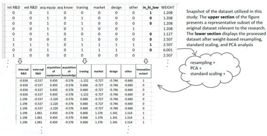
Figure 1.
Comparative visualization of the dataset before and after pre-processing, including weight-based resampling, standardization, and Principal component analysis.
2.2. Experimental Setup
2.2.1. Model Selection
To comprehensively evaluate the predictive performance of different machine learning algorithms for binary classification tasks, seven models were selected: Logistic Regression, Random Forest, Gradient Boosting (specifically XGBoost, LightGBM, and CatBoost), Support Vector Machines (SVMs), and Artificial Neural Networks (ANNs) using a multi-layer perceptron classifier architecture. This collection of models spans both classic (e.g., Logistic Regression, Random Forest, SVM) and modern ensemble or deep learning approaches (e.g., XGBoost, LightGBM, CatBoost, ANN), thus offering a diverse testbed for performance comparisons across various complexities of function approximation. By including regularized linear models, tree-based ensembles, kernel methods, and neural networks, the experimental design captures a broad spectrum of hypothesis spaces, ensuring robust insights into which methods excel under differing data conditions.
A key motivation for selecting these models lies in their complementary strengths: for instance, Logistic Regression often provides interpretable coefficients, Random Forest and Gradient Boosting methods can capture complex interactions through ensembles, SVMs are effective in high-dimensional spaces with appropriate kernel design, and ANNs can approximate non-linear relationships given sufficient training data. Moreover, these seven models are commonly used as baselines or benchmarks in predictive analytics, making them well-suited for a comparative study aimed at identifying the most effective modeling strategies for innovation outcome prediction.
2.2.2. Model Construction and Relevant Parameters
Each algorithm requires a specific set of hyperparameters, and the selected hyperparameter optimization is shown in Table 1. The defined abbreviations from Table 1 will be used later in the presentation of the final results of the hyperparameter tuning process as well as in the general naming of the models.

Table 1.
Selected hyperparameters for ML models.
Hyperparameters regulate various aspects of the learning process. For instance, Logistic Regression includes parameters such as the choice of solver, penalty (L1, L2, or none), regularization strength C, and maximum number of iterations. Random Forest and Gradient Boosting frameworks (XGBoost, LightGBM, and CatBoost) include parameters controlling tree depth, learning rates, subsampling, and regularization. Support Vector Machines involve kernel types, penalty parameter C, and kernel-specific parameters. Artificial Neural Networks encompass solver type, hidden layer configurations, activation functions, regularization coefficients, and other optimization settings (e.g., batch size, learning rate).
These hyperparameters ultimately shape the model’s bias-variance trade-off, its computational cost, and predictive capacity. The next section describes how the hyperparameters are tuned via cross-validation and a special optimization procedure to obtain models that are best suited for the subsequent performance evaluations.
2.3. Hyperparameter Tuning and Model Evaluation
2.3.1. Hyperparameter Optimization Approaches
To systematically select hyperparameters for each model, stratified k-fold cross-validation was employed. Stratification preserves the class distribution in every fold, mitigating the risk of model bias toward a particular class distribution, which is especially crucial in binary classification problems [28]. Moreover, k-fold cross-validation offers a reliable estimate of model performance by rotating the training and validation sets through each fold. A consistent random seed was used to ensure the reproducibility of these splits. Cross-validation was chosen in lieu of a simple train-validation-test partition because it maximizes data usage for both training and validation, reducing variance in estimates of model performance.
Multiple hyperparameter optimization techniques were explored—manual tuning, grid search, random search, nested cross-validation, and Bayesian optimization. Nested cross-validation provides an unbiased performance estimate by nesting an inner optimization loop within an outer cross-validation loop [29]. However, this approach proved excessively time-consuming given the extensive search space across numerous models and parameters. Consequently, Bayesian Optimization (implemented via Hyperopt, without nesting) emerged as the primary optimization strategy, balancing search efficiency with overall computational cost [30].
Hyperopt utilizes probabilistic models to explore the hyperparameter space, typically yielding superior performance in fewer iterations than exhaustive methods [31]. This method employs the Tree-structured Parzen Estimator (TPE) to adaptively sample promising regions of the parameter space, often discovering near-optimal configurations without the prohibitive time investment required by more exhaustive search methodologies. A custom search space was defined for each model, encompassing both integer and continuous parameters while accounting for conditional dependencies (i.e., certain hyperparameters became active only when specific model settings were chosen).
2.3.2. Implementation Details and Constraints
To achieve the best-fitting hyperparameters for subsequent performance evaluations, two distinct tuning sessions were performed—one using 10-fold cross-validation (10×-CV) and another using 5 × 2 cross-validation (5 × 2-CV)—so that each model ultimately has two sets of optimized hyperparameters. Throughout tuning, regularization played an important role wherever applicable (e.g., L1- and L2-penalties or their combinations). Regularization helps prevent overfitting by penalizing overly complex models, thereby improving generalization [13]. For instance, Logistic Regression, XGBoost, LightGBM, and CatBoost (among others) support L1 (lasso-type) and/or L2 (ridge-type) penalties; including these settings in the search space improved model resilience against noisy features.
In designing the Bayesian optimization boundaries, certain parameter interactions were carefully constrained to reflect known model requirements. For instance, in Random Forest, the choice of ‘max_features’ influences how many features are randomly selected at each split. Similarly, in CatBoost, enabling certain grow policies or adjusting the ‘leaf_estimation_iterations’ must remain consistent with the chosen learning rate. By defining conditional search spaces, Hyperopt effectively navigated these complexities, yielding model-specific hyperparameter sets that delivered both high predictive performance and improved computational efficiency.
All hyperparameter tuning trials were conducted on identical hardware configurations and software versions, with uniform random seeds ensuring repeatability in all comparisons. Detailed hyperparameter ranges for each model (e.g., solver types, penalty mechanisms, search bounds for regularization coefficients) can be found in Table 2. This uniformity of the process across all models guarantees that the observed differences in performance can be attributed to model characteristics and not to inconsistent experimental conditions.
Table 2.
Hyperparameter ranges for Hyperopt tuning across selected models.
In the Table 2 ‘Hyperparameter Ranges’ column, the notation specifies the nature of the search space for each parameter. Values enclosed in brackets ([]) indicate that the search space consists of the explicitly listed discrete values. When the notation includes log(range), the parameter values are sampled logarithmically across the specified range. If the range is defined as n1–n2, the search space includes all continuous values between n1 and n2, inclusive. For ranges denoted as n1–n2’K, the search space is limited to discrete steps of size K within the specified range from n1 to n2.
2.4. Performance Metrics
A rigorous statistical framework was adopted to compare machine learning models for predicting innovation outcomes, encompassing careful selection of performance metrics, cross-validation procedures, and a structured evaluation method. By incorporating multiple quantitative indicators, the analysis aimed to capture the multidimensional nature of model performance and support robust, reproducible findings [32,33].
Performance was assessed through well-established metrics, each emphasizing a particular aspect of predictive accuracy and practical utility. Accuracy, defined as the proportion of correctly classified instances, provided a baseline measure but could obscure issues arising from class imbalance. Precision, the fraction of true positives among predicted positives, was integral for scenarios where false alarms or misclassifications imposed high costs. Recall (sensitivity) quantified the proportion of actual positives correctly identified, a key consideration when failing to detect important signals—such as potential breakthroughs—can be costly. The F1 score, as the harmonic mean of precision and recall, underscored the trade-offs inherent in imbalanced data. Finally, the area under the receiver operating characteristic curve (ROC-AUC) served as an overarching indicator of a model’s discriminatory power by aggregating its performance across varying thresholds [34]. Employing these metrics in tandem ensured that the comparative analysis of machine learning algorithms provided a holistic perspective on predictive efficacy in the context of innovation outcomes.
2.5. Power Analysis
A statistical power analysis was initially conducted to ascertain the minimum sample size required for the reliable evaluation and comparison of machine learning models aimed at predicting innovation outcomes. Prior to performing the comparative tests, this analysis was applied to verify whether the data produced through cross-validation or resampling procedures would be sufficient for detecting meaningful differences in model performance. In particular, all methods—except for McNemar’s test—depended on data derived from either 5 × 2 or K-fold cross-validation; accordingly, it was imperative to determine whether the common practice of obtaining K data points would furnish adequate statistical power.
To ensure adequate estimates, Cohen’s d and the required sample size were calculated based on results obtained from 100 repeated 10-fold cross-validation (in a total of 1000 splits). This approach was employed to enhance the reliability of the estimates by considering the variability across a substantial number of splits.
To estimate the effect size, Cohen’s d was calculated by dividing the mean difference in performance by the corresponding standard deviation. This standardized metric captured the magnitude of discrepancies among models. The significance level (α) was set to 0.05, and a statistical power of 0.8 was targeted to mitigate the likelihood of Type II errors. A two-sided alternative hypothesis was adopted to accommodate potential differences in either direction, thereby enabling a comprehensive evaluation of model performance. This methodological design permitted the determination of a suitable sample size for identifying substantive performance variations, and the power analysis was performed separately for each metric and each of the aforementioned methods.
Determining the appropriate sample size is crucial for constructing dependable machine learning models, and power analysis serves as a statistical framework for estimating the minimum sample size necessary to detect an effect of a specified magnitude with a given degree of confidence. Nonetheless, when implementing K-fold cross-validation, the assumption of independence between training and validation sets is violated because each data point is used in both stages across different folds. This interdependence can complicate the straightforward application of conventional power analysis techniques. Despite this complication, the power analysis remains a valuable practice, as it provides a baseline estimate of the sample size needed to attain sufficient statistical power. Once this baseline has been established, the use of repeated K-fold cross-validation can enhance the rigor of model assessment by further probing the stability and robustness of the results.
2.6. Statistical Analysis
Multiple evaluation techniques were employed to address the acknowledged absence of a single definitive approach for determining which machine learning model performs best and by what margin [19]. The selection of statistical tests was guided by prior research, highlighting the need to minimize both Type I (false positive) and Type II (false negative) errors in comparative analyses. As a result, a suite of advanced statistical methods—namely, the 5 × 2 cross-validation paired t-test, the 10-fold cross-validation paired t-test, the Wilcoxon non-parametric pairwise signed-rank test, the corrected random resampled t-test, the corrected k-fold cross-validation t-test, the corrected repeated k-fold cross-validation t-test, McNemar’s test, and the non-parametric Friedman test—was incorporated to evaluate performance across metrics including accuracy, precision, recall, F1-score, and ROC-AUC.
Cross-validation remains one of the most prevalent methods for model evaluation, particularly in cases with limited data availability [28]. However, K-fold cross-validation is known to exhibit high variability, which can lead to erratic behavior in estimated prediction errors and potentially misleading outcomes during model selection [18]. Moreover, there is no unbiased estimator of the variance in K-fold cross-validation, nor is there conclusive theoretical support indicating that any existing bias becomes negligible when the sample size is not asymptotically large [19]. In light of these concerns, multiple evaluation techniques—along with the correction strategies proposed by Nadeau and Bengio [20] and by Bouckaert and Frank [21]—were adopted to mitigate the impact of correlation within training and test folds [35]. Such an integrative approach was deemed critical to reducing the risk of misleading conclusions by leveraging complementary insights from distinct evaluation procedures. Consequently, a multifaceted approach was deemed necessary to mitigate these biases and ensure that performance differences among models could be more reliably detected.
The 5 × 2 cross-validation paired t-test was chosen due to its relatively low risk of Type I error, as suggested by empirical studies [18]. Although it does not fully eliminate the correlation introduced by reusing training and test splits within the same procedure, its iterative structure—consisting of five repetitions of twofold splits—offers a practical balance between computational feasibility and variance control. Nevertheless, generating only 10 metric points in this design can yield insufficient statistical power, as preliminary power analyses indicated that approximately 100 measures would be optimal, thereby suggesting that the Type II error rate may be appreciably elevated. Consequently, the 5 × 2 cross-validation t-test should be interpreted with caution, particularly regarding its ability to detect subtle yet potentially meaningful performance differences.
The 10-fold cross-validation paired t-test, by contrast, is associated with a higher Type I error rate but offers greater sensitivity when detecting performance differences. Notwithstanding, this approach also tends to produce a relatively limited number of aggregated measurements, which can reduce its overall statistical power. Despite these constraints, it was included in the present study owing to its frequent use in the literature, where it is often preferred for balancing computational efficiency and the need for comparative performance assessment.
The Wilcoxon non-parametric pairwise signed-rank test was additionally employed to address potential violations of normality assumptions. This test was performed on the performance estimates derived from the 10-fold cross-validation procedure and from ten times repeated 10-fold cross-validation (100 aggregate measurements). Because the Wilcoxon test does not rely on strict parametric assumptions, it provides a robust alternative for detecting model differences under distributional irregularities.
To further account for the correlation among repeated measures, three corrected methods introduced by Nadeau and Bengio [20] and by Bouckaert and Frank [21] were integrated [35]. A corrected random resampling t-test was performed by randomly partitioning the dataset into training (67%) and test (33%) subsets across 100 iterations, while a corrected K-fold cross-validation t-test followed the traditional 10-fold design with the applied correction from Nadeau and Bengio. The corrected repeated K-fold cross-validation t-test extended this approach through ten repetitions of 10-fold cross-validation, producing a total of 100 performance estimates. These correction algorithms adjust conventional variance estimators to better capture the dependencies arising from repeated usage of the same data folds, thereby enhancing the reliability of the resulting statistical inferences.
McNemar’s test was applied to compare two classifiers based on matched pairs of outcomes. This test is well-suited for assessing performance differences when the same instances are evaluated by both models because it focuses on the consistency of misclassifications. By examining whether one classifier tends to misclassify instances that the other classifier labels correctly—and vice versa—McNemar’s test furnishes a robust way to detect statistically significant differences in model performance [18]. In addition, McNemar’s test is less influenced by distributional assumptions than certain parametric methods and therefore serves as a valuable tool when the goal is to compare the proportions of errors directly. Unlike the conventional application of McNemar’s test to a single train/test split, this study implemented a repeated McNemar test across multiple data splits (10-fold-CV-splits). This approach ensures a more robust and generalizable assessment of performance differences by aggregating the results across several train/test configurations, thus mitigating the sensitivity and variability introduced by any single partition.
Finally, the Friedman test was employed on the aggregated results from the 10 repeated 10-fold cross-validation experiments (100 estimates). As a non-parametric test, the Friedman procedure does not rely on assumptions of normality and is particularly appropriate for comparing more than two algorithms across multiple datasets or folds. This method ranks the performance of each algorithm on each fold and evaluates whether observed rank differences are statistically significant. Owing to its ability to handle multiple models simultaneously without requiring normally distributed performance metrics, the Friedman test is frequently recommended for comprehensive model comparisons in machine learning research. If statistically significant differences are detected, follow-up post hoc analyses (e.g., the Nemenyi or Bonferroni-Dunn test) can be performed to identify which pairs of models differ meaningfully.
2.7. Software and Tools
The computational framework for this study was built in Python (version 3.12.0), chosen for its robust ecosystem of data science libraries and straightforward syntax. Several key frameworks and libraries were employed to implement and evaluate our machine learning models. Specifically, ‘scikit-learn’ (version 1.5.2) [36] served as the foundational toolkit for model construction, evaluation, and cross-validation routines [1]. In tandem with ‘scikit-learn’, the gradient boosting libraries ‘xgboost’ (version 2.1.1) [37], ‘lightgbm’ (version 4.5.0) [38], and ‘catboost’ (version 1.2.7) [39] were utilized to harness their state-of-the-art performance characteristics, particularly beneficial for tabular datasets.
To optimize model hyperparameters, we leveraged the ‘hyperopt’(version 0.2.7) [40] package, employing the Tree-structured Parzen Estimator (TPE) for Bayesian optimization. Within each Bayesian optimization routine, the ‘cross_val_score’ function from ‘sklearn.model_selection’ was used to fine-tune each model’s hyperparameters by maximizing the F1 score. For the final model evaluations based on multiple train–test splits, the ‘cross_validate’ function from ‘sklearn.model_selection’ enabled consistent and reproducible cross-validation performance metrics.
Statistical power analyses to determine appropriate sample sizes were conducted using ‘ttestindpower’ from ‘statsmodels.stats.power’ (version 0.14.4) [41]. Moreover, we employed functions from ‘mlxtend.evaluate’ (version 0.23.1) [42]—namely, ‘paired_ttest_5 × 2cv’ and ‘paired_ttest_kfold_cv’—to perform statistical tests across cross-validation folds, providing greater rigor in performance comparisons. For the assessment of classification model misclassifications, the ‘mcnemar_table’ and ‘mcnemar’ [42] methods were harnessed to conduct the McNemar test. Finally, for conducting non-parametric analyses such as the Friedman and Wilcoxon tests, we utilized the ‘friedmanchisquare’ and ‘wilcoxon’ functions from ‘scipy.stats’ (version 1.14.1) [43].
To address the issue of inflated Type I error rates associated with traditional statistical tests on correlated samples, the ‘correctipy’ package (commit 99cc7e87 from GitHub) [35] was incorporated into the computational framework of this study. This Python package is designed to implement corrected test statistics specifically tailored for scenarios involving non-independent samples, such as those generated through resampling and k-fold cross-validation procedures. Within ‘correctipy’, the functions ‘resampled_ttest’, ‘kfold_ttest’, and ‘repkfold_ttest’ were utilized to perform statistical comparisons between machine learning models. Modifications were applied to all the aforementioned functions to enhance the accuracy and validity of the statistical analyses. Discrepancies, such as the absence of a square root operation in the denominator of the t-statistic computation or similar straightforward errors, were identified. These issues were corrected to align the computations with the appropriate statistical methodology. All machine learning models were constructed using a consistent random seed (random state = 39) to ensure full reproducibility of results across experiments and mitigate variability due to stochastic processes inherent in model initialization and data partitioning.
All computational experiments were performed on an HP-250-G7 Notebook PC, powered by an Intel64 Family 6 Model 142 CPU operating at 2300 MHz and equipped with 16 GB of RAM. The training times and hyperparameter optimization durations for each model were recorded on this hardware configuration and will be reported in the subsequent results section.
3. Results
In this chapter, the results of hyperparameter tuning are presented first, including the final parameters used to train and test each model. Statistical power analysis is then presented to determine the minimum sample size required to reliably evaluate and compare the performance of machine learning models. Leveraging these optimized parameters, the statistical results are then reported. Descriptive statistics and performance comparisons for metrics such as test accuracy, test F1, test ROC AUC, and fit time follow. Finally, the results of the statistical analyses are provided, encompassing the t-test using 5 × 2 cross-validation, the t-test on 10-fold cross-validation data, the McNemar test conducted on the entire dataset, and the Friedman test applied to the results of 10-fold cross-validation.
3.1. Hyperparameter Tuning Resutls
The hyperparameter tuning experiments yielded insights into model performance and computational requirements under two cross-validation (CV) approaches—10-fold cross-validation (10× CV) and 5 × 2 cross-validation (5 × 2 CV)—across all seven machine learning algorithms included in this study: Artificial Neural Networks (ANN), Random Forest (RF), Logistic Regression (LR), Support Vector Machines (SVM), LightGBM (LGBM), CatBoost (CB), and XGBoost (XGB). The fine-tuned hyperparameters for each model are reported in Table 3.
Table 3.
Summary of final hyperparameter configurations for ML models tuned with 10-fold and 5 × 2 cross-validation procedures.
Figure 2 illustrates the hyperparameter tuning time per trial for the 10-fold CV and 5 × 2 CV approaches accordingly. The chart reveals that Random Forest and CatBoost models incurred noticeably higher tuning times with the 5 × 2 CV compared to the 10× CV approach, indicating that models exhibiting greater complexity or sensitivity to data partitioning may experience additional computational overhead due to different train/test split ratios. By contrast, Logistic Regression, SVM, and LightGBM produced minimal differences in tuning time between the two referent strategies, reflecting the stability and lower complexity of these algorithms. Unlike the other models—where tuning times for 10× CV were generally lower than those for 5 × 2 CV—ANN and XGBoost models exhibited slightly higher tuning times for 10× CV compared to 5 × 2 CV.
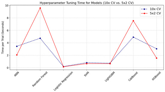
Figure 2.
Analysis of computational overhead in hyperparameter tuning times for 10× CV and 5 × 2 CV methods across ML models.
Figure 3 presents the optimal loss values (negative performance metric) obtained during the hyperparameter tuning process for each model. The performance metric used in the tuning process is the F1 score for the optimization. However, it is represented as a negative value because the Hyperopt algorithm minimizes the objective function during the search for the optimal parameter configuration. Consequently, lower loss values indicate better performance.

Figure 3.
Best loss (−F1 scores) for ML models during hyperparameter tuning”.
CatBoost, for instance, achieved the best loss under 10× CV (approximately −0.812) with a ‘depth’ parameter of six and a ‘learning rate’ of 0.116, while under 5 × 2 CV, its performance decreased moderately to −0.791. A similar trend was noted in XGBoost, where 10× CV yielded −0.807 but declined to −0.784 with fewer training samples per fold. ANN also benefited from the larger training set, achieving −0.807 when two hidden layers were employed under 10× CV, although a simpler single-layer design under 5 × 2 CV maintained competitive performance at −0.792.
3.2. Power Analysis Resutls
While power analysis is not inherently required for comparing machine learning (ML) models—largely due to the violations of independence in cross-validation and resampling—it can still serve as a valuable tool to gain deeper insights into the adequacy of sample sizes for robust model evaluation. By quantifying the variability in sample size requirements across different performance metrics and model pairs, power analysis provides a structured framework for addressing two critical challenges in ML research: determining the optimal dataset size for reliable comparisons and understanding the limitations of statistical power under practical constraints.
Pairwise effect sizes and corresponding power analyses revealed that substantially larger sample sizes would be desirable to attain adequate statistical power than initially ten estimates anticipated, as shown in Table 4, which presents the pairwise median calculated sample sizes across all metrics for referent models. If we take averages for a particular metric into consideration, variations are even more extreme. For example, the average proposed sample size for the accuracy metric for certain pairs (RF/LGBM and RF/ANN) was over five thousand when all model pairs were considered, while the calculated mean sample size for accuracy was 189 (including all models). Comparable disparities were observed across all other metrics, with certain model pairs necessitating only modest sample sizes (for example, LR pairs) while others demanded exceedingly large ones. The exact median calculated sample sizes for the referent metrics (including all models) were as follows: accuracy (189), precision (38), recall (43), F1-score (268), and ROC AUC (19). These results underscore the variability in sample size requirements depending on the performance metric under consideration.
Table 4.
Median sample sizes derived from power analysis across models (all metric).
To simplify the research process, the sample size was standardized to 100 for all subsequent analyses. This choice was informed primarily by two considerations. First, the median required sample sizes for most metrics clustered around or below 100, making it a suitable upper bound for ensuring sufficient power in a broad range of comparisons. Second, using a uniform sample size streamlined the design of robust comparative tests without incurring prohibitive computational overhead.
Due to the differing requirements of statistical tests, two complementary evaluation schemes were finalized: one offering 10 performance estimates per model (via 5 × 2 cross-validation and single-run 10-fold cross-validation) and another producing 100 estimates per model (using ten repeated 10-fold cross-validation and corrected random resampling with 100 splits). The Friedman and Wilcoxon tests were similarly adapted to operate on 100 estimates (and for 10 as well), thereby facilitating more reliable multiple-model comparisons.
By balancing established (10-split) and enhanced (100-split) procedures, it is anticipated that a more comprehensive and robust assessment of model performance will be obtained. Adopting 100 estimates supports the substantial variability in required sample sizes observed in the power analysis while offering a feasible pathway to improved statistical rigor.
3.3. Descriptive Statistics
In Figure 4 and Table 5, the descriptive statistics of the performance of all examined models (Random Forest, ANN, Logistic Regression, SVM, LightGBM, CatBoost, and XGBoost) are presented for all considered metrics (Accuracy, Precision, Recall, F1-Score, and ROC-AUC). These statistics were computed under two cross-validation protocols: the conventional 10-fold cross-validation, providing 10 estimates (represented by red bars), and a 10-times repeated 10-fold cross-validation, yielding 100 estimates (illustrated by blue bars). (To maintain clarity, results for the 5 × 2 cross-validation procedure are not displayed in Figure 4 but can be found in Figure 3).
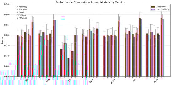
Figure 4.
Benchmarking models (test set) by metrics (Accuracy, Precision, Recall, F1, ROC-AUC) with standard deviations.
Table 5.
Model Performance (test set) by Metrics with 95% Confidence Intervals (Z = 1.96, sample size 10 and 100) for 10-fold CV and repeated 10-fold CV evaluation.
When the two approaches are compared, it is apparent that their outcomes are relatively consistent, although the repeated cross-validation procedure produces slightly lower results on average. Moreover, for all models except SVM, the ROC-AUC metric values deviate substantially from the mean trends observed in the other metrics. It should also be noted that the Logistic regression model performs worse on all metrics and that its results show the highest variability within the metric as well as a higher standard deviation compared to the other models. This higher variance is likewise evident in Table 5, which provides confidence intervals among other statistical details.
Additionally, the LightGBM model yields the most stable results for the majority of metrics—aside from ROC-AUC—reporting values around 0.80, thereby indicating a relatively robust and consistent performance profile.
3.4. Statistical Tests
3.4.1. McNemar’s Test
The McNemar’s test was employed to assess statistically significant differences in classification performance across referent models—Random Forest (RF), Artificial Neural Network (ANN), Logistic Regression (LR), Support Vector Machine (SVM), LightGBM (LGBM), CatBoost (CB), and XGBoost (XGB)—(Table 6). A pronounced divergence was observed in all pairwise comparisons involving LR, which exhibited consistent underperformance relative to other models, as evidenced by universally significant p-values (p < 0.001) and elevated chi-squared statistics (e.g., χ2 = 47.70 vs. RF; χ2 = 50.08 vs. ANN; χ2 = 54.28 vs. CB). These results underscore LR’s inferior discriminative capacity within the evaluated framework.
Table 6.
Pairwise McNemar’s Test Analysis of Classifier Performance: Chi-Square Statistics and Statistical Significance (p-Values).
Statistically significant differences (α = 0.05) were further identified exclusively in two pairwise comparisons: CB versus RF (p = 0.0315, χ2 = 4.63) and CB versus LGBM (p = 0.0036, χ2 = 8.49). The absence of significance in the CB-XGB comparison (p = 0.210) was noted, with the chi-squared value reported as ‘nan’, a condition typically arising when contingency table cells contain zero counts, precluding conventional test computation. This outcome, however, aligns with the non-significant p-value derived via exact binomial approximation, suggesting parity in classification efficacy between CB and XGB.
3.4.2. 5 × 2 Cross-Validation Paired t-Test
A pairwise 5 × 2 cross-validation paired t-test was conducted to evaluate all model pairs included in this research, and the resulting outcomes are presented in Table 7, which is divided into two parts. The lower triangular section of Table 7, situated below the main diagonal, provides the total count of detected statistically significant differences (p < 0.05) across the five examined performance metrics (accuracy, precision, recall, F1-score, and ROC-AUC) for each model pair. For instance, the cell corresponding to the Random Forest (RF) and Logistic Regression (LR) comparison contains the value 5, indicating that statistically significant performance gaps (p < 0.05) were identified for all five metrics under the 5 × 2 paired t-test. This figure can range from a maximum of 5 to a minimum of 0, with zeros omitted from the table to ensure readability. The upper triangular region of Table 7, located above the main diagonal, displays letters corresponding to the metrics for which a statistically significant difference emerged for a given pair of models: A for Accuracy, P for Precision, R for Recall, F for F1-score, and C for ROC-AUC. Uppercase letters (A, P, R, F, C) denote instances where the column-based model (model1) significantly outperforms the row-based counterpart (model2), while lowercase letters (a, p, r, f, c) indicate the opposite, where model2 outperforms model1. In the previously mentioned RF/LR example, the upper cell lists all five lowercase letters, implying that the LR model significantly underperformed the RF model on every measured metric. This nomenclature remains consistent across further statistical tests and is therefore not elaborated again. Complete statistical test results for all pairs/models, including exact t-scores and p-values, are available in Appendix A Table A1.
Table 7.
Aggregate pairwise performance of 5 × 2 CV paired t-test.
The conducted 5 × 2 CV paired t-test revealed that all comparisons involving Logistic Regression (LR) produced statistically significant differences (p < 0.05). This outcome corroborates the findings in both Figure 3 and Table 5, which indicate that Logistic Regression yields considerably poorer classification performance relative to the other methods. The statistical test has now confirmed that the visibly weaker performance of LR, observed in earlier tables and figures, is robust to formal hypothesis testing. Among other model comparisons, Support Vector Machine (SVM) was found to differ significantly from several counterparts on the ROC-AUC metric, while no statistically significant differences were detected for SVM under the remaining metrics.
Across the accuracy metric, LR was significantly outperformed by all models (for instance, on RF vs. LR: t = 6.3684, p = 0.0014; ANN vs. LR: t = 7.4070, p = 0.0007; CB vs. LR: t = 5.2129, p = 0.0034). Inspection of precision revealed similar patterns; for example, LR showed a t-score of 4.1429 (p = 0.0090) relative to RF and a t-score of 5.5737 (p = 0.0026) when tested against CB. Under the recall metric, the disadvantages of LR were again confirmed by statistically significant comparisons such as XGB vs. LR (t = 2.0102, p = 0.0034) and SVM vs. LR (t = 2.9035, p = 0.0337). The F1 results underpin the general weakness of LR, with p-values (typically below 0.03) for all pairs, for example, (RF vs. LR: t = 5.4417, p = 0.0028; CB vs. LR: t = 3.9013, p = 0.0114, etc.). Finally, ROC-AUC analyses provided particularly strong evidence for LR’s weakness, as seen in RF vs. LR (t = 8.5058, p = 0.0004), LGBM vs. LR (t = 9.1800, p = 0.0003), and XGB vs. LR (t = 7.6399, p = 0.0006).
Under ROC-AUC, the SVM demonstrated inferior performance. Comparative analyses against models such as RF, LGBM, and CB frequently resulted in statistically significant differences, as indicated by small p-values and relatively large t-scores. These findings suggest that SVM’s ranking capability deviated substantively from that of its counterparts (except LR), highlighting potential limitations in its discriminative effectiveness within the given classification framework (for example, RF vs. SVM: t = 4.8027, p = 0.0049; LGBM vs. SVM: t = 5.8171, p = 0.0021; XGB vs. SVM: t = 6.3247, p = 0.0015). By contrast, other metrics did not show marked differences for SVM when tested against the same methods. These findings are consistent with the graphical depictions in Figure 3, which illustrated a noticeable inferiority for SVM under the ROC-AUC metric performance.
The overall impression is that most classifiers outside of LR did not differ significantly from one another across multiple measures, but that SVM stands out in its area-under-curve behavior, while LR sits at a clear disadvantage on virtually every metric.
3.4.3. 10-Fold Cross-Validation Paired t-Test
The results of the pairwise 10-fold cross-validated paired t-test are presented in Table 8, which summarizes the number of statistically significant differences across all models and all pairs evaluated in this study. Full and detailed 10-folc-CV results are shown in Appendix A Table A2.
Table 8.
Aggregate pairwise performance table for 10-fold CV paired t-test.
A substantially higher number of performance differences was observed compared to the 5 × 2 cross-validation test, with statistically significant differences detected across nearly all model pairs—where at least one metric exhibited significance. An exception was noted for the XGBoost/CatBoost (XGB/CB) pairing, where no differences were identified across any metrics.
The disparities were predominantly concentrated in pairs involving the Logistic Regression (LR) model, which demonstrated systemic deficiencies in performance relative to other algorithms. However, the 10-fold CV paired t-test also highlighted discrepancies in pairs containing CatBoost (CB), with CB exhibiting discriminative superiority over multiple counterparts, whereas LR consistently ranked as the lowest-performing model (Table 5).
Under the accuracy metric, CB exhibited a consistently superior performance, shown by its significantly better outcomes against most of the competing models. Although XGB approached CB with no conclusive difference established between them (t = 1.707 p = 0.122), suggesting comparable accuracy levels. Logistic Regression, on the other hand, ranked consistently lower (with a t-score around and above 5) than the other methods and showed significant inferiority in the vast majority of pairwise comparisons. Other models demonstrated intermediate performance, frequently producing accuracy scores that were neither statistically distinguishable from the leading methods nor markedly superior or definitively inferior.
With respect to precision, three algorithms—ANN, CB, and XGB—emerged as top performers. Their pairwise comparisons did not yield statistically significant disparities, indicating that they occupied a similar performance tier. Each of these three methods, however, significantly surpassed RF, LR, SVM, and LGBM in multiple tests.
The recall results differ from the patterns observed in accuracy and precision. The SVM proved to be the most outstanding model for this metric, recording a significantly higher recall than most of its counterparts. RF also demonstrated moderately high recall (RF vs. ANN, t = 2.949, p = 0.016, RF vs. LR, t = 14.933, p < 0.001), and it did not differ significantly from certain strong competitors like CB, XGB, SVM, and LGBM. Logistic Regression performed poorly once more, losing decisively against the majority of comparisons.
CB achieved prominent F1 scores, significantly surpassing many competing classifiers, including RF, ANN, LR, and LGMB. However, the differences between CB and certain other methods were statistically insignificant, suggesting that SVM and XGB perform at a comparable level for F1. Evaluation under the ROC-AUC metric indicated that CB, XGB, and ANN each occupied the top tier without significant differences among them. These methods were uniformly more effective than RF, LR, and SVM in multiple comparisons. LGBM performed acceptably but lagged behind the leading group, suggesting that CB and XGB offered the strongest separation capacity.
3.4.4. Corrected 10-Fold Cross-Validation Paired t-Test
The summarized results for the corrected version of the 10-fold cross-validation method, as proposed by [24,35], are presented in Table 9, while the complete statistical data for all pairwise comparisons and metrics are provided in Appendix A (Table A3).
Table 9.
Aggregate performance table of Corrected 10-fold cross-validation paired t-test.
The corrected 10-fold CV test effectively reduces bias and Type I error, leading to a lower number of model pairs exhibiting statistically significant differences compared to the standard 10-fold CV test. However, the overall pattern remains consistent, with the logistic regression (LR) model demonstrating clear inferiority across all evaluated metrics.
RF occupied a mostly inferior position across all metrics. It showed notable superiority over LR in all metrics, for example, on accuracy (t = 6.967, p < 0.001) and precision (t = 2.787, p = 0.005), while no statistically significant differences were detected against ANN in most comparisons except on ROC-AUC (t = −4.140, p < 0.001), where it underperforms. However, CB consistently surpassed RF on almost all metrics (except recall) on accuracy (t = −4.783, p < 0.001) and precision (t = −4.461, p < 0.001), and XGB likewise outperformed RF in precision (t = −2.797, p = 0.005) and ROC-AUC (t = −4.552, p < 0.001). RF on most metrics statistically does not differ from SVM but has better performance on ROC-AUC (t = 3.923, p < 0.001). Overall, RF was neither conclusively the best nor the worst, frequently ranking in the mid-lower tier.
ANN demonstrated strong performance across multiple metrics, outperforming SVM (t = 2.888, p = 0.004) and LGBM (t = 2.020, p < 0.043) on precision, as well as surpassing SVM on ROC-AUC. However, it underperformed relative to SVM in recall (t = −12.188, p < 0.001). ANN significantly outperformed LR across all metrics, including ACC (t = 7.090, p < 0.001) and PREC (t = 4.338, p < 0.001). Comparisons with CB and XGB revealed no statistically significant differences (e.g., ACC: ANN vs. CB, t = −0.696, p = 0.486), indicating that while ANN ranks among the stronger classifiers, it does not decisively outperform the top models.
LGBM demonstrated statistically significant inferior performance in the vast majority of cases where differences were identified, with the exception of RF and SVM on the ROC-AUC metric and LR across all metrics. CB outperformed LGBM on four out of five metrics, while XGB showed superiority on three out of five. ANN achieved a statistically significant advantage only in precision (t = −2.020, p = 0.043), whereas no statistically significant differences were observed in other pairwise comparisons involving these models.
SVM demonstrated notable strengths in recall, outperforming all models except RF. It significantly surpassed leading classifiers such as CB (t = 3.329, p = 0.001) and XGB (t = 3.786, p < 0.001) and, in certain instances, RF, although this difference did not reach statistical significance (p = 0.107). Across all other metrics, SVM either underperformed or yielded statistically insignificant differences, with the exception of LGBM, where it exhibited a significant advantage on the F1 metric (t = 2.547, p = 0.011).
CB emerged as one of the strongest classifiers across nearly all metrics, demonstrating significant advantages wherever statistical differences were identified, except against SVM in recall. It outperformed RF on four out of five metrics, LR on all metrics, and LGBM on all but recall, where the difference was statistically insignificant (t = 0.455, p = 0.649) but still in the same direction. Comparisons with XGB and ANN generally did not reach significance (e.g., XGB accuracy: t = 1.046, p = 0.296; ANN precision: t = 0.405, p = 0.685), suggesting that CB, XGB, and ANN occupy a similarly strong position among top-performing models.
XGB likewise ranked among the best performers, particularly rivaling CB and ANN. It consistently outperformed LR in all five metrics (e.g., accuracy: t = 8.457, p < 0.001; precision: t = 5.121, p < 0.001, etc.). The comparisons with CB on accuracy and ROC-AUC showed no significant gap (t = −1.046, p = 0.296; t = −0.518, p = 0.604), suggesting an equivalently strong capacity. Similarly, with ANN model pairs, XGB did not find any statistical superiority. XGB held advantages over RF (precision: t = −2.797, p = 0.005; ROC-AUC: t = −4.552, p < 0.001), affirming its position as a consistent top-tier method across the examined metrics. Also, it statistically outruns three out of five metrics in comparison with LGBM.
LR consistently lagged behind its counterparts across accuracy, precision, recall, f1, and ROC-AUC. It was decisively outperformed by RF (accuracy: t = −6.967, p < 0.001; precision: t = −2.787, p = 0.005) and ANN (accuracy: t = −7.090, p < 0.001; precision: t = −4.338, p < 0.001). Comparisons against CB, ANN, and XGB likewise revealed statistically significant disadvantages, with p-values below 0.001 in most pairwise tests. These patterns indicate that LR occupied the lowest tier among the evaluated models.
3.4.5. Corrected Repeated (Ten-Times) 10-Fold Cross-Validation Paired t-Test
Unlike the previous analysis of the corrected 10-fold CV test, this statistical evaluation is based on 100 estimates derived from 10 repetitions of 10-fold CV with different splits, thereby increasing statistical power. The summarized results for the pairwise corrected-repeated 10-fold CV paired t-test, as proposed by Bouckaert and Frank [21], are presented in Table 10, while the complete statistical data for all pairwise comparisons and metrics (including p-values and t-scores) are provided in Appendix A (Table A4).
Table 10.
Aggregate performance of Corrected 10x repeated 10-fold-CV paired t-test.
As shown in Table 10, the results align closely with those of the previous corrected 10-fold CV test (Table 9), maintaining a consistent overall pattern, particularly in the dominance significance difference count among LR, SVM, and RF model pairs.
LR consistently occupied the lowest tier, with highly significant disadvantages (p < 0.001) against all other models on every metric. Its performance gap was particularly evident in accuracy (e.g., LR vs. ANN: t = 6.1035, p < 0.0001) and ROC-AUC (LR vs. CB: t = −9.9764, p < 0.0001).
RF did not exhibit significant differences from most models in accuracy or F1. However, it was statistically outperformed in precision by CB (t = −3.6917, p = 0.0004), ANN (t = −2.9728, p = 0.0037), and XGB (t = −3.3647, p = 0.0011). In recall, RF ranked among the top alongside SVM (no significant difference, p = 0.1702), yet in ROC-AUC it was surpassed by CB, XGB, and ANN (all p ≤ 0.0008).
SVM demonstrated a pronounced advantage in recall, significantly surpassing CB, XGB, and LGBM (p ≤ 0.001). Its lead over RF was not conclusive (p = 0.170). Nonetheless, for precision and ROC-AUC, SVM was consistently outperformed by ANN, CB, and XGB (p < 0.001 in most pairwise comparisons). For the remaining SVM pairwise comparisons across metrics (excluding LR), no statistically significant differences were observed. However, regarding the F1 metric, while no significant differences were detected, SVM exhibited a dominant tendency. This is reflected in its positive t-scores when compared to top-performing models such as CB (t = 0.348, p = 0.728) and XGB (t = 0.490, p = 0.625).
ANN ranked among the top three for precision (e.g., ANN vs. SVM: t = 2.9467, p = 0.0040) and ROC-AUC, where it was statistically indistinguishable from CB and XGB (all p > 0.0937). Meanwhile, it shared no notable differences with RF and LGBM in accuracy or F1, implying a strong yet not dominant position. Regarding RF and SVM, ANN exhibited mixed results, outperforming RF on certain metrics while underperforming on others, such as recall. However, ANN demonstrated a clear advantage over LGBM in cases where statistical differences were identified, including precision (t = 2.151, p = 0.034) and ROC-AUC (t = 2.448, p = 0.014).
LGBM showed no significant gaps from the high-performing models on accuracy (e.g., LGBM vs. CB: p = 0.1244, LGBM vs. XGB: p = 0.1893). However, in precision and ROC-AUC, it was eclipsed by ANN, CB, and XGB (p ≤ 0.034). Its F1 performance remained on par with other classifiers except LR.
CB and XGB consistently emerged as leading classifiers across most metrics. Neither displayed significant superiority over the other (all p ≥ 0.8158 in precision; p = 0.9001 in ROC-AUC), and both attained strong positions in accuracy and precision. Their outperformance of LR, RF, and SVM reached statistical significance in multiple comparisons (e.g., XGB vs. LR in precision: t = 4.0168, p < 0.0001; CB vs. SVM in precision: t = 4.3526, p < 0.0001). Regarding ANN, no statistically significant results indicate its outperformance; however, the t-values suggest a tendency toward inferiority in opposition to CB and XGB.
Overall, LR was conclusively the weakest, while CB and XGB formed a top tier alongside ANN in precision and ROC-AUC. SVM and RF excelled primarily in recall, whereas LGBM maintained competitive yet slightly less dominant results.
3.4.6. Corrected Random Resampled Cross-Validation Paired t-Test
The corrected random resampled CV paired t-test, proposed by Nadeau and Bengio [20], was introduced to mitigate the Type I error inherent in the classical resampled CV paired t-test, which has been shown to exhibit increasing bias as the number of repetitions grows. Similar to repeated 10-fold cross-validation, this corrected test generated 100 estimates, aligning with the recommendations of statistical power analysis to ensure sufficient power and minimize the risk of Type II error.
The summarized pairwise results are presented in Table 11, while a detailed breakdown of the statistical test, including t-scores and p-values, is provided in Appendix A (Table A5). The results reveal a structure consistent with previous analyses, particularly the corrected 10-times repeated 10-fold CV paired t-test (Table 10), with most statistically significant differences observed among LR, SVM, and RF model pairs.
Table 11.
Aggregate performance table of Corrected random resampled paired t-test.
Test again affirmed that LR performed significantly worse than all other models across all metrics (e.g., accuracy vs. RF: t = −4.769, p < 0.001; precision vs. CB: t = −3.591, p < 0.001; recall vs. XGB: t = −3.384, p = 0.001), consistently positioning it at the lower tier.
Regarding accuracy, all classifiers except LR displayed mostly comparable results, with no statistically significant differences observed among RF, ANN, SVM, LGBM, CB, and XGB (e.g., ANN vs. CB: p = 0.444; CB vs. XGB: p = 0.888). In contrast, for precision, CB and XGB exhibited significant advantages over RF (p = 0.020 and p = 0.027, respectively) as well as over SVM and LGBM. The recall results underlined the dominance of SVM, which outperformed ANN, LGBM, CB, and XGB (p < 0.05 in each pairwise test) and also significantly outperformed LR. Meanwhile, in the F1-score, all models except LR formed a statistically indistinguishable result. Lastly, ROC-AUC analyses confirmed the overall strength of CB and XGB, as each surpassed RF and SVM (e.g., CB vs. RF: t = −3.915, p < 0.001; XGB vs. SVM: t = −4.064, p < 0.001) and did not significantly differ from each other (p = 0.1789). ANN also showed good results under the ROC-AUC metric, outperforming RF (t = 2.129, p = 0.036) and SVM (t = 4.065, p < 0.001). In sum, CB, XGB, and ANN formed a top-performing cluster, RF, SVM, and LGBM resided in a lower and mid-range position, and LR consistently placed at the lower bound of the comparative evaluation.
3.4.7. Wilcoxon Non-Parametric Signed-Rank Test
In addition to the parametric paired t-test, the Wilcoxon pairwise non-parametric signed-rank test was conducted to ensure more robust results, addressing potential violations of normality assumptions, small sample sizes, and the influence of outliers. Unlike the t-test, the Wilcoxon test operates on rank values rather than raw numerical differences, allowing it to capture consistent directional differences between models even when absolute values vary.
The aggregated results are presented in Table 12, while the full set of detailed statistical results is available in Appendix A (Table A6). The results indicate a substantially higher number of statistically significant pairwise differences compared to the t-test. Notably, the test identified significant differences (in at least three metrics) for nearly all model pairs, with the sole exception of CB and XGB, where no statistically significant difference was detected.
Table 12.
Aggregate performance table for non-parametric Wilcoxon signed-rank test (100 estimates) results across multiple metrics.
The sample for the Wilcoxon test was derived from repeated 10-fold cross-validation, resulting in 100 estimates. Initially, two approaches were considered: a standard 10-fold CV (yielding 10 estimates) and a repeated 10-fold CV (yielding 100 estimates). The latter was selected as it better aligns with the sample size requirements determined by statistical power analysis. With a sample size of only 10, the results were considerably more modest in terms of detecting statistically significant differences (higher Type II error).
Which model performs better cannot be derived directly from the W value, as this is always a positive value (unlike the t value). Instead, the medians of the model outputs are compared in order to take account of the rank-based nature of the Wilcoxon test. From Table 12, it is evident that CB and XGB once again dominate across nearly all metrics and model comparisons, with the exception of the recall metric, where SVM, RF, and LGBM demonstrate stronger performance. As observed in previous analyses, SVM maintains its dominance in recall across all model pairs. Additionally, in the F1 metric, SVM outperforms all models except CB and XGB, where no statistically significant difference is observed, making it inconclusive which model has the advantage. ANN, RF, and exhibit mixed results, while LR consistently ranks as the weakest performer, surpassing only RF on a few metrics and ANN on ROC-AUC.
3.4.8. Non-Parametric Friedman Test
All previously applied statistical methods have been pairwise comparison tests, aiming to identify statistically significant differences between specific model pairs. The results were presented in tables, each populated with the outcomes of all possible two-model comparisons. In contrast, the Friedman test employs a multiple-model comparison approach, simultaneously evaluating all models to provide a broader perspective on their relative performance.
As a non-parametric test, the Friedman test imposes no prior assumptions about the input distribution. Its results indicate whether a statistically significant difference exists among the tested models; however, it does not specify which models differ. To determine specific pairwise differences, a post-hoc test, such as Nemenyi’s test, is required.
The Friedman test was performed using 100 estimates per metric, obtained through a repeated cross-validation procedure to ensure alignment with the required sample size. The statistical results, including chi-square values and p-values, are presented in Table 13. Across all metrics, statistical significance was achieved with p < 0.001, and the large chi-square values (>480) provide strong evidence of performance differences among models. The highest chi-square value was observed for ROC-AUC (568.36), while the lowest was recorded for the recall metric (481.6).
Table 13.
Results of Friedman test across multiple metrics.
Table 14 presents a summary of performance results across multiple metrics in the same format as previously shown. The results closely resemble those obtained from the corrected repeated cross-validation t-test (Table 10) and the corrected resampled t-test (Table 11). The most statistically significant differences were identified for the LR model, followed by SVM, LGBM, and RF. The table further highlights the dominance of CB and XGB across most metrics, except for recall, while LR consistently underperforms across all metrics. Additionally, SVM maintains its superiority in recall over all models except RF, where no statistically significant difference was observed.
Table 14.
Summary performance table for Friedman non-parametric pairwise test (100 estimates).
A complete set of results for all model-metric combinations, including exact p-values from Nemenyi’s post-hoc test, is provided in Table A7 (Appendix A).
Table 15 presents a summary of the average rankings of different classification models across various metrics. Each model was evaluated 100 times, with the corresponding metric computed in each iteration. Rather than using raw scores, models were ranked per iteration, with 1 assigned to the best-performing model for a given metric and 7 to the worst. After 100 iterations, the average rankings were calculated and are displayed in Table 15. The results indicate that LR is the poorest-performing model, consistently ranking above 6 across all metrics. In terms of accuracy, precision, and ROC-AUC, the best performing models are CB (2.71, 2.39, 1.90) and XGB, which have slightly higher rankings. ANN follows closely behind, with an average value of rankings around 3. However, SVM is the best model for recall and F1, followed by CB and XGB. These findings align with previous observations regarding recall (Table 8, Table 9, Table 10 and Table 11) and F1 (Table 12), reinforcing the overall ranking trends. Additionally, RF demonstrated strong performance in recall and F1 metrics, securing second and third place rankings, respectively.
Table 15.
Rank aggregation table on 100 estimates across multiple metrics.
The rankings in Table 15, in contrast to those in Table 14, are average ranks without statistical tests or significance analyzes. To conclude this evaluation, the Friedman statistical test followed by the post-hoc Nemenyi test is graphically presented in Figure 5 in the form of critical difference (CD) diagrams, providing a visual comparison of model performance across multiple metrics.
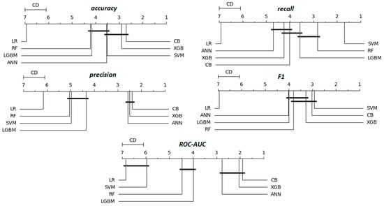
Figure 5.
Critical difference diagrams from Friedman Test with Nemenyi post-hoc analysis by metrics (accuracy, precision, recall, F1, ROC-AUC).
In the critical difference (CD) diagram for accuracy (Figure 5), four distinct performance groups of ML models can be observed. The top-performing group consists of CB and XGB (positioned on the right side of the scale), followed by a middle group comprising SVM and ANN. A lower-middle group includes RF and LGBM, while LR stands as a clear outlier on the far-left side of the chart, indicating the worst performance.
For precision, three performance groups can be identified: CB, XGB, and ANN as the top-performing models; RF, SVM, and LGBM forming a middle-tier group; and LR again positioned as the lowest-performing model on the far left. The ROC-AUC metric follows a similar grouping pattern, except that SVM shifts from the middle group to the lower-performing group alongside LR, while RF and LGBM remain in the middle tier.
In recall, LR continues to exhibit the worst performance, whereas SVM emerges as the best-performing model by a significant margin. The middle-tier models are more evenly distributed, with RF and LGBM showing the strongest results, followed by CB and XGB. ANN, in contrast, performs poorly on this metric.
For F1, the top-performing group consists of SVM, CB, and XGB, while RF, LGBM, and ANN cluster closely together in the middle tier. As expected, LR remains the worst-performing model.
It is important to note that the black lines connecting models in the CD diagrams indicate that no statistically significant difference exists between the grouped models for the selected metrics. For example, in the precision metric sub-chart, CB, XGB, and ANN are not statistically different in performance, just as RF, LGBM, and SVM form a statistically indistinguishable group.
4. Discussion
4.1. Hypothesis
The evaluation of seven machine learning models was undertaken to investigate whether their algorithmic distinctions would yield significant differences in performance when predicting innovation outcomes based on company innovation activities. Consistent with hypothesis H1 (“Machine learning models applied to predict innovation outcomes based on company innovation activities will exhibit differential performance across key predictive metrics, largely driven by each model’s inherent algorithmic properties and alignment with the dataset.”), the results of all statistical tests provide solid support. Significant performance disparities were consistently observed, and no single test failed to reject the null hypothesis for at least one pair of models, indicating that the choice of algorithm is indeed consequential in this predictive context.
In contrast, hypothesis H2 (“Ensemble learning methods (Random Forest, XGBoost, CatBoost, and LightGBM) will yield superior predictive performance compared to individual models (Linear Regression, SVM, and ANN) in forecasting innovation outcomes from firm-level innovation activities.”) received only partial empirical support. Although CatBoost and XGBoost emerged as top performers across most metrics, SVM demonstrated superior recall, underscoring that certain individual models can excel in specific performance dimensions. Random Forest and LightGBM, while generally slightly less effective than CatBoost and XGBoost, also achieved comparatively strong recall values (as evidenced by the Friedman test in Figure 5). Consequently, these findings do not unequivocally affirm hypothesis H2, since the ensemble methods did not uniformly surpass the non-ensemble models across all predictive metrics.
With respect to hypothesis H3 (“CatBoost will outperform other gradient boosting algorithms (XGBoost and LightGBM) owing to its efficient handling of categorical variables, resulting in improved innovation outcome predictions.”), the comparative evaluation of CatBoost against XGBoost and LightGBM yielded findings that favor CatBoost over LightGBM with statistical significance. Multiple tests, including the Friedman test (for nearly all metrics except recall, where no significant difference was identified, see Figure 5), McNemar’s test (Table 6), the 10-fold CV paired t-test (Table 8), and the corrected 10-fold CV paired t-test (Table 9), consistently demonstrated that CatBoost performed significantly better than LightGBM. In contrast, the difference between CatBoost and XGBoost was statistically insignificant in most tests, although CatBoost showed a small but not statistically significant promotional advantage. Furthermore, CatBoost displayed better average performance metrics and average ranks (Table 15, Figure 5) when compared directly to XGBoost. Consequently, these results indicate that CatBoost outperformed the other gradient boosting models, thereby confirming Hypothesis H3.
Regarding Hypothesis H4 (“Artificial Neural Networks (ANNs) will not significantly surpass simpler models (e.g., Linear Regression and SVM) in predicting innovation outcomes, primarily due to the limited size and binary nature of the dataset.”), partial support was observed. Although ANN consistently surpassed Linear Regression in almost all metrics across every statistical test (Table 6, Table 7, Table 8, Table 9, Table 10, Table 11, Table 12, Table 13 and Table 14), the comparison between ANN and SVM yielded more nuanced outcomes. Most tests indicated that ANN excelled over SVM in terms of precision and ROC-AUC (Table 7, Table 8, Table 9, Table 10, Table 11, Table 12, Table 13 and Table 14). However, ANN underperformed relative to SVM in the recall metric in almost all cases and also underachieved on the F1 metric (as shown by the Wilcoxon signed-rank test in Table 12 and the Friedman test in Figure 5). These mixed findings suggest that neither ANN nor SVM unequivocally dominated across all evaluation criteria. In contrast, ANN demonstrated a clear advantage over Linear Regression, thus providing evidence that ANN can outperform at least one simpler model in a statistically significant manner. As a result, Hypothesis H4 cannot be fully accepted, given that ANN did indeed significantly outperform Linear Regression.
Finally, Hypothesis H5 (“Logistic Regression (LR) will be the most computationally efficient model among those examined, given its relatively simple structure and reduced computational demands compared to more complex algorithms.”) was evaluated based on overall training, tuning, and inference times. Although a dedicated statistical test was not performed for computational efficiency, Figure 2 (chapter “Hyperparameter tuning results) clearly illustrates that Logistic Regression was the fastest model during hyperparameter tuning (Bayesian search over 1000 iterations on multiple cross-validation schemes) and model fitting. In Figure 6 (above), Logistic Regression exhibited the shortest average fit (training) time (0.0131 s), followed by LightGBM (0.0452 s), and also achieved the fastest scoring time (0.0169 s), with ANN (0.0177 s) and CatBoost (0.0182 s) closely behind. These results confirm that Logistic Regression maintains the fastest execution throughout training, testing, scoring, and tuning, thereby validating Hypothesis H5.
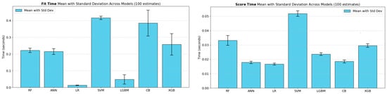
Figure 6.
Comparison of model execution times: mean fit and score times with standard deviation across machine learning models (100 estimates).
4.2. Hyperparameter Tuning Time & Performance
For executing ML models and conducting statistical tests, hyperparameter tuning was performed to optimize both the 5 × 2 cross-validation procedure (used for the 5 × 2 CV paired t-test) and the 10-fold cross-validation approach (applied to all other statistical tests, except for the resampled test).
To obtain 100 estimates, repeated 10-fold cross-validation with varying splits was conducted, ensuring alignment with the optimized hyperparameters for 10-fold CV. The only deviation from this optimized setup occurred in the corrected random resampled cross-validation paired t-test, where data splits followed a 66:34 ratio instead of the standard 90:10 used in other 10-fold cross-validation procedures. As a result, hyperparameters may not be fully optimized for this specific test.
To analyze tuning time in relation to hyperparameter optimization results (Figure 2), a significant variation in tuning duration (time per trial) across different ML models can be observed. Notably, Random Forest and CatBoost require less tuning time under the 10-fold cross-validation procedure compared to the 5 × 2 cross-validation approach, whereas ANN and XGBoost exhibit the opposite trend, requiring more time for 10-fold cross-validation, regardless of the fact that both methods involve the same total number of training and testing iterations (10 in total).
However, the computational cost is not solely determined by the number of cycles; it also depends on the size of the training sets per each cycle. The size of the training and test sets differs between the two methods, which can impact computational time. In 10-fold cross-validation, each training set comprises 90% of the data, and each test set comprises 10%. In 5 × 2 cross-validation, each training set comprises 50% of the data, and each test set also comprises 50%. Training on larger datasets generally requires more computational time.
Therefore, the larger training sets in 10-fold cross-validation should lead to longer training times per iteration compared to 5 × 2 cross-validation. However, the specific machine learning algorithm used can influence the computational time. Some algorithms scale differently with the size of the training data, which can affect the overall time required for cross-validation. This trade-off between smaller but repeated folds (5 × 2 CV) and larger single-fold partitions (10× CV) highlights the importance of aligning cross-validation selection with model complexity and resource availability.
Furthermore, in terms of hyperparameter tuning performance for F1 (Figure 3), it was observed that 10-fold cross-validation generally yielded slightly better results. This improvement is likely attributed to the larger proportion of training data per fold, which facilitated more effective generalization. Random Forest exhibited a relatively smaller performance difference, but it required significantly more time under 5 × 2 cross-validation due to the repeated use of data and its tendency to favor deeper ensemble structures. The smallest gap in performance between 5 × 2 cross-validation and 10-fold cross-validation was observed in the Logistic Regression model, likely because it is less sensitive to variations in training data size due to its simplicity and lower risk of overfitting compared to more complex models.
4.3. Statistical Results
Following the descriptive statistical analysis (Figure 4, Table 5—Chapter Results/Descriptive Statistics), a comparison was conducted between the results obtained from standard 10-fold cross-validation (10 estimates) and 10-times repeated 10-fold cross-validation (100 estimates) across various performance metrics, including accuracy, precision, recall, F1, and ROC-AUC.
The findings indicate that, on average, the results obtained from 100 estimates (folds) were slightly worse than those from the standard 10-fold CV (10 estimates). This discrepancy may be attributed to the effect of random variation, which, while introducing greater variability, can also lead to a more robust and generalized performance estimate.
Single 10-fold CV relies on a specific partition of the data, which may inadvertently favor the model due to random splits that include “easier” test examples. Repeated 10-fold CV averages over multiple partitions, reducing the influence of chance and providing a more stable estimate of model performance. This aligns with findings that repeated cross-validation decreases variance in performance estimates and better approximates the true generalization error [18]. Another possible explanation is that repeated cross-validation introduces variability in the composition of test sets, which may expose the model to more challenging instances or less favorable class distributions. Bengio & Grandvalet (2003) emphasize that repeated data splits can inadvertently create test sets with different underlying distributions compared to a single split, potentially leading to lower performance metrics while simultaneously enhancing the robustness and realism of the evaluation [19].
Furthermore, as observed in Figure 4, the ROC-AUC metric consistently outperforms other evaluation metrics across all ML models, with an approximate 10% improvement. For instance, CatBoost achieves accuracy, precision, recall, and F1 scores around 0.80, while its ROC-AUC reaches 0.87. This pattern is evident across all models, except for SVM, where the difference between ROC-AUC and other metrics is less pronounced.
The reason can be that metrics like accuracy, precision, and F1 depend on a fixed decision threshold (often 0.5), while ROC-AUC evaluates the model’s ability to rank positive instances above negatives across all possible thresholds. A model with well-separated class probabilities (e.g., CatBoost, XGBoost) may have suboptimal performance at the default threshold but strong ranking capability, leading to a higher ROC-AUC. This aligns with Fawcett (2006), who emphasizes that AUC measures “the probability that a classifier will rank a randomly chosen positive instance higher than a negative one”, independent of threshold choice [34]. One more reason can be that SVM might be less “probabilistic”. Standard SVMs output uncalibrated decision values (distances to the hyperplane) rather than true probabilities. Without post-processing (e.g., Platt scaling), these scores lack the spread and calibration needed to exploit threshold variations, narrowing the gap between ROC-AUC and threshold-based metrics. Niculescu-Mizil & Caruana (2005) show that SVMs require explicit calibration to produce reliable probabilities, and uncalibrated scores often cluster near the decision boundary, limiting their threshold adaptability [44]. This explains why SVM’s ROC-AUC and threshold metrics may align more closely than probabilistic models like CatBoost or logistic regression.
Further analysis of the McNemar test and the paired 5 × 2 cross-validation t-test reveals that their conservative nature—manifesting in fewer statistically significant differences compared to other methods—stems from their inherent methodological properties. McNemar’s test focuses on discordant pairs. McNemar’s test evaluates differences in model performance by analyzing only the disagreements between two models (i.e., instances where one model is correct and the other is wrong). This narrow focus reduces sensitivity to small but consistent performance differences across the entire dataset, leading to fewer significant results compared to tests that consider all observations. Dietterich (1998) notes that McNemar’s test has lower statistical power in scenarios where performance differences are subtle but widespread [18].
The paired 5 × 2 CV t-test uses a limited number of folds (5 repeats of 2-fold splits) to estimate variance, which can lead to overly conservative error estimates. Alpaydin (1999) showed that this test’s strict variance correction reduces Type I error rates (false positives) but also decreases power, making it harder to detect significant differences unless the effect size is large [45]. In contrast, tests like corrected repeated CV or Wilcoxon may overestimate significance due to less rigorous variance handling.
Regarding the elevated Type I error in resampled and repeated cross-validation tests, Dietterich (1998) highlights that the resampled t-test is prone to increased Type I error due to the non-independence of training sets within cross-validation. (same logic can be applied to repeated k-fold cross-validation), making it unreliable. The classical resampled t-test’s inflated error arises because it ignores dependencies between training folds, leading to overly optimistic significance estimates [18].
The corrected random resampled CV paired t-test, proposed by Nadeau and Bengio (2003), adjusts the variance estimate to account for overlapping training data, mitigating this issue and providing valid Type I error control [20]. Additionally, the corrected repeated 10-fold cross-validation method was employed in this study to mitigate Type I error.
4.4. Limitations
It must be acknowledged that the chosen approach is primarily based on supervised learning algorithms (ANN, SVM, LR, RF, LightGMB, XGBoost, and CatBoost) and thus excludes potential insights from unsupervised or semi-supervised methods. Although principal component analysis (PCA) was used during data preprocessing to explore the dimensional structure of the input space, this method was not applied as a stand-alone approach to uncover latent clusters or reveal novel groupings among the firms. The focus on these seven supervised models was based on their proven interpretability and their ability to achieve the classification objective of distinguishing between high- and low-innovative firms. Nevertheless, the exclusive focus on supervised classification is a clear limitation, as further integration of unsupervised methods (e.g., clustering or advanced dimensionality reduction) could potentially reveal deeper structural insights and improve the overall understanding of innovation-related outcomes.
An important limitation—which has been pointed out multiple times—is the dependency between training and test sets when performing statistical tests using k-fold cross-validation, repeated cross-validation, and resampled cross-validation to obtain the required number of estimates for statistical evaluation. Although this approach is widely used, it is important to recognize this problem, and that is why new methods have been proposed to mitigate this effect, such as corrected k-fold, corrected repeated k-fold, and corrected resampled k-fold cross-validation.
Another limitation of this study results from the variability of the required sample size determined by the power analysis, which varied considerably depending on the model pair and the evaluation metric used. The required sample size ranged from less than five for LR model pairs (for most metrics, with the exception of the precision metric) to over ten thousand for certain model comparisons. For example, in the case of XGB vs. CB on ROC-AUC—where performance differences were minimal—the power analysis yielded a required sample size of 29,442. For all metrics (accuracy, precision, recall, F1, and ROC-AUC), the median required sample size was 192, while the average was 1446. An optimal approach would be to generate a required number of estimates for each pair of models on each metric, based on the results of the power analysis. However, this would significantly increase computational complexity and resource requirements. Therefore, a uniform number of 100 estimates was chosen for this study, which strikes a practical balance between feasibility and statistical rigor, although this remains a limitation.
In addition, the McNemar’s statistical test uses multiple iterations instead of a single run. Traditionally, the McNemar’s test is applied to a benchmark test set (e.g., 10% of the sample in a single split). However, in this study, predictions were made across the entire dataset using a k-fold approach (‘cross_val_predict’), violating the assumption of independence between training and test sets. This change was made to increase the number of data points and mitigate the effects of fluctuations in small subsamples, albeit at the cost of some bias. Nevertheless, the results of the McNemar’s test (Table 6) show that it remains very conservative and primarily identifies statistically significant differences in comparisons with LR models while revealing far fewer differences than other statistical tests. This suggests that the approach did not substantially inflate the Type I error rate, which emphasizes the robustness of the results. Another limitation of this study is that it relies on a two-tailed approach for all statistical tests, which detects significant differences in both directions. As the hypotheses were specifically designed to test whether certain models were superior to others, a one-sided approach would have been more appropriate. Using this method could have resulted in a greater number of statistically significant differences being identified than the two-sided approach used.
4.5. Choosing Appropriate Models: Practical Scenarios
An exhaustive guide to model selection was not the main objective of the present study. Nevertheless, the results obtained allow some practical recommendations. If a high recall is a priority, the SVM or a carefully tuned ensemble method (e.g., CatBoost or XGBoost) can be used to capture as many positive instances as possible. In scenarios requiring balanced performance in terms of other metrics, CatBoost and XGBoost have consistently achieved good results, including robust ROC-AUC values. In situations where limited computational resources are available, logistic regression proved to be particularly suitable due to its short training and inference times compared to the other algorithms evaluated. Therefore, practitioners are advised to base model selection on the specific performance metrics of interest (e.g., precision, recall, F1, ROC-AUC), available computational capacity, and the inherent distribution of the dataset.
4.6. Future Research
Null-hypothesis significance tests (NHST), used in this paper, highlight critical challenges in interpreting classifier comparisons. NHST frameworks, such as the signed-rank and correlated t-tests, often conflate statistical significance with practical relevance. For instance, p-values—central to NHST—are influenced by both effect size and sample size, which can lead to rejecting the null hypothesis even for negligible differences between classifiers when datasets are sufficiently large [46,47,48]. Moreover, NHST cannot affirmatively support the null hypothesis; it merely fails to reject it, leaving ambiguity about whether classifiers are truly equivalent [49]. These shortcomings underscore the need for alternative methodologies that provide more nuanced insights into classifier performance. Future research could address these limitations by adopting Bayesian approaches, which enable probabilistic interpretations of effect sizes and explicitly incorporate regions of practical equivalence (ROPE) to distinguish meaningful differences from trivial ones.
A promising direction lies in the Bayesian hierarchical modeling framework proposed by Corani et al. (2017) [24], which overcomes key NHST constraints. Unlike traditional NHST, their approach allows simultaneous inference on both dataset-specific effects (δi) and the population-level effect (δ0), offering a holistic view of classifier performance across multiple datasets. By leveraging Bayesian principles, researchers can quantify evidence for or against hypotheses, rather than relying on binary rejections of the null. For example, the Bayesian correlated t-test [50] computes posterior distributions of effect sizes, enabling direct probability statements about classifier superiority, equivalence, or practical insignificance. Extending such methods to hierarchical models—as in Corani et al. (2017)—would further enhance generalizability by pooling information across datasets while accounting for variability. Future studies adopting this framework could yield more robust, interpretable conclusions, aligning statistical outcomes with practical relevance in classifier evaluation [24].
In addition to the methodological innovations, an equally important avenue for future research is to broaden the scope of the data sources examined. Although the present study focuses on a single dataset from the Community Innovation Survey (CIS2014) with a particular focus on Croatia, the Community Innovation Survey itself covers a wide range of European countries and sectors, each surveyed according to harmonized guidelines. This provides valuable opportunities for cross-country analyses comparing how machine learning models work on innovation data in different institutional or economic contexts. Similarly, a breakdown by industry—using standardized classifications such as NACE codes—could show whether certain algorithmic approaches have higher predictive power in specific sectors characterized by different rates of technological adoption or market competition. The inclusion of additional data from Eurostat or other official statistical agencies would thus facilitate more comprehensive tests of the generalizability of the models and allow researchers to determine whether the observed performance trends persist across different regions or industries. These extensions, in conjunction with the Bayesian approaches mentioned above, have the potential to form a comprehensive framework that evaluates and compares machine learning classifiers in a setting that extends well beyond the boundaries of a single region or dataset.
It should be noted that the present work focuses on the study of performance metrics and relative computation times using medium-sized data. While the observed patterns give a reasonable indication of how these algorithms might behave, real large environments may have other nuances, such as higher memory usage, network overhead in distributed environments, or nonlinear scalability. Future research could examine these models on much larger datasets to clarify how the resource consumption of each algorithm scales, providing more detailed guidance on balancing performance and computational requirements.
5. Conclusions
In this work, multiple machine learning algorithms—both ensemble-based and single-model approaches—were applied to a firm-level innovation dataset to predict which companies would achieve higher innovation intensity. Tree-based boosting methods were found to perform consistently well on several metrics, notably accuracy, F1, precision, and area under the ROC curve, while a kernel-based method performed best on recall. This divergence suggests that no single algorithm dominates in all performance measures but that different algorithmic strengths emerge depending on the aspect of prediction accuracy being evaluated.
Implementation details showed that models using boosting frameworks were slightly more resource intensive but provided superior discriminative power on many classification metrics, while simpler methods generally provided faster computations with moderate accuracy. Therefore, the pragmatic decision of which algorithm to use should be determined by a trade-off between computational effort and the relative importance of specific performance goals (e.g., maximizing sensitivity versus balancing overall accuracy).
Methodologically, various statistical procedures were used to determine that significant performance differences exist between the compared models. Cross-validation procedures were combined with corrections for repeated use of the same data, which reduced the risk of inflated Type I error rates. Nevertheless, it was found that results can fluctuate if the variance arising from overlapping folds is not carefully accounted for. The interplay between the size of the training set, the repetition strategies, and the complexity of the model also highlighted the importance of robust experimental designs that take into account computational cost, sample size, and methodological rigor.
Although one class of ensemble algorithms was found to be particularly reliable, it is possible that domain-specific variations in data structure or class distribution could favor other techniques. Future analyzes that integrate Bayesian methods, hierarchical modeling, and additional qualitative insights into firms’ innovation processes could provide even more accurate or interpretable predictions. By systematically fitting models to both data features and desired performance criteria, stakeholders can optimize resource allocation and maximize the potential impact of machine learning in shaping innovation outcomes.
Author Contributions
Conceptualization, M.M. and D.P.; methodology, M.M. and K.D.; software, M.M. and K.D.; validation, M.M., K.D., and D.P.; formal analysis, M.M.; investigation, K.D.; resources, D.P.; data curation, K.D.; writing—original draft preparation, M.M.; writing—review and editing, K.D. and D.P.; visualization, M.M. and D.P.; supervision, D.P.; project administration, D.P. All authors have read and agreed to the published version of the manuscript.
Funding
This research received no external funding.
Data Availability Statement
The data that support the findings of this study are subject to restrictions and are not publicly available due to confidentiality and legal agreements. The data used in this research are third-party data from the Community Innovation Survey (CIS) 2014, managed by Eurostat. Access to these data can be requested directly from Eurostat or relevant national statistical offices. Detailed information about the application process for accessing CIS microdata is available at https://ec.europa.eu/eurostat/web/microdata/community-innovation-survey (accessed on 1 December 2024).
Conflicts of Interest
The authors declare no conflict of interest.
Abbreviations
The following abbreviations are used in this manuscript:
| A | Alpha (regularization parameter for ANN) |
| ACC | Accuracy |
| AI | Artificial Intelligence |
| ANN | Artificial Neural Networks |
| AT | Activation (function)—hyperparameter in ANN (e.g., ReLU, Tanh) |
| AUC | Area Under the Curve (generic term) |
| B1 | Beta1 (exponential decay rate for the first moment estimates in Adam optimizer) |
| B2 | Beta2 (exponential decay rate for the second moment estimates in Adam optimizer) |
| BS | Batch Size (hyperparameter for ANN training) |
| BT | Bagging Temperature (CatBoost hyperparameter) |
| C | (1) Regularization strength (penalty parameter) in Logistic Regression/SVM(2) In the statistical tables, sometimes used to denote “ROC-AUC” |
| CB | CatBoost |
| CD | Critical Difference (in post-hoc tests/diagrams after Friedman test) |
| CIS | Community Innovation Survey |
| CIS2014 | Community Innovation Survey 2014 (Croatian sample used in the paper) |
| CL | Colsample ByLevel (XGBoost hyperparameter) |
| CPU | Central Processing Unit (hardware) |
| CT | Colsample ByTree (XGBoost/LightGBM hyperparameter) |
| CV | Cross-Validation (general term) |
| D | (1) Depth (CatBoost hyperparameter)(2) Degree (SVM polynomial kernel hyperparameter) |
| E | Epsilon (e.g., for Adam optimizer in ANN, or for SVM tolerance in some contexts) |
| EM | Eval Metric (CatBoost hyperparameter) |
| ES | Early Stopping (ANN hyperparameter) |
| F1 | F1-score (classification metric, harmonic mean of precision & recall) |
| FF | Feature Fraction (LightGBM hyperparameter) |
| GP | Grow Policy (CatBoost hyperparameter) |
| G | Gamma (SVM or XGBoost hyperparameter, depending on context) |
| HLS | Hidden Layer Sizes (ANN hyperparameter) |
| I | Iterations (CatBoost hyperparameter) |
| k-fold | K-Fold Cross-Validation (general CV technique) |
| K | Kernel (SVM hyperparameter, e.g., ‘rbf’, ‘poly’, ‘linear’) |
| L1 | Lasso penalty (L1 regularization) |
| L2 | Ridge penalty (L2 regularization) |
| L2R | L2 Leaf Reg (CatBoost hyperparameter for leaf regularization) |
| LGBM | LightGBM (gradient boosting library/model) |
| LEI | Leaf Estimation Iteration (CatBoost hyperparameter) |
| LR | (1) Logistic Regression (model) in the main text and tables(2) Learning Rate (hyperparameter) in boosting/ANN contexts |
| MCW | Min Child Weight (XGBoost hyperparameter) |
| MD | Max Depth (common tree-based hyperparameter for RF, XGB, LGBM, etc.) |
| MDL | Min Data in Leaf (LightGBM, CatBoost hyperparameter) |
| MDS | Max Delta Step (XGBoost hyperparameter) |
| MF | Max Features (Random Forest hyperparameter) |
| MI | Max Iterations (hyperparameter for LR, SVM, ANN) |
| ML | Machine Learning |
| MSE | Mean Squared Error |
| MS | Max Samples (Random Forest hyperparameter) |
| MSG | Min Split Gain (LightGBM hyperparameter) |
| MSS | Min Samples Split (Random Forest hyperparameter) |
| MSL | Min Samples Leaf (Random Forest hyperparameter) |
| NHST | Null-Hypothesis Significance Tests (general statistical framework) |
| N | Estimators (number of trees/estimators, e.g., in RF, XGB, LGBM) |
| OOB | Out-of-Bag (Random Forest hyperparameter) |
| p | p-value (statistical significance measure) |
| P | Penalty (hyperparameter in Logistic Regression) |
| PCA | Principal Component Analysis |
| RA | Reg Alpha (XGBoost/LightGBM hyperparameter) |
| RAM | Random Access Memory (hardware) |
| RF | Random Forest |
| RL | Reg Lambda (XGBoost/LightGBM hyperparameter) |
| ROC | Receiver Operating Characteristic |
| ROC-AUC | Area Under the Receiver Operating Characteristic Curve (same as AUC-ROC) |
| RS | Random Strength (CatBoost hyperparameter) |
| RSM | Random Subspace Method (CatBoost hyperparameter) |
| S | Solver (hyperparameter for LR, ANN) |
| SVM | Support Vector Machines |
| SS | Subsample (XGBoost, LightGBM, CatBoost hyperparameter) |
| T | Tolerance (hyperparameter for SVM and ANN) |
| TPE | Tree-structured Parzen Estimator (Bayesian optimization method used by Hyperopt) |
| V | Verbose (LightGBM hyperparameter) |
| VF | Validation Fraction (ANN hyperparameter) |
| XGB | XGBoost (gradient boosting library/model) |
| 5 × 2 CV | 5-times 2-fold Cross-Validation procedure |
| 10× CV | 10-fold Cross-Validation (sometimes written simply as “10-fold CV”) |
Appendix A
Table A1.
Pairwise 5 × 2-CV paired t-test results across multiple metrics (T-score/p-value).
Table A1.
Pairwise 5 × 2-CV paired t-test results across multiple metrics (T-score/p-value).
| Accuracy | RF | ANN | LR | SVM | LGBM | CB | XGB |
|---|---|---|---|---|---|---|---|
| RF | — | 0.213/(0.840) | 6.368/(0.001) | nan/(0.000) | 1.364/(0.231) | 0.627/(0.558) | 1.431/(0.212) |
| ANN | −0.213/(0.840) | — | 7.407/(0.001) | −0.104/(0.921) | 0.969/(0.377) | 0.395/(0.709) | 1.645/(0.161) |
| LR | −6.368/(0.001) | −7.407/(0.001) | — | −3.584/(0.016) | −3.388/(0.020) | −5.213/(0.003) | −3.664/(0.014) |
| SVM | nan/(0.000) | 0.104/(0.921) | 3.584/(0.016) | — | 1.586/(0.174) | 0.464/(0.662) | 1.880/(0.119) |
| LGBM | −1.364/(0.231) | −0.969/(0.377) | 3.388/(0.020) | −1.586/(0.174) | — | −1.232/(0.273) | 0.251/(0.812) |
| CB | −0.627/(0.558) | −0.395/(0.709) | 5.213/(0.003) | −0.464/(0.662) | 1.232/(0.273) | — | 1.218/(0.278) |
| XGB | −1.431/(0.212) | −1.645/(0.161) | 3.664/(0.014) | −1.880/(0.119) | −0.251/(0.812) | −1.218/(0.278) | — |
| Precision | RF | ANN | LR | SVM | LGBM | CB | XGB |
| RF | — | −0.133/(0.899) | 4.143/(0.009) | −2.020/(0.099) | 0.430/(0.685) | −0.549/(0.607) | −0.792/(0.464) |
| ANN | 0.133/(0.899) | — | 2.456/(0.058) | −0.495/(0.642) | 0.474/(0.656) | −0.333/(0.753) | −0.385/(0.716) |
| LR | −4.143/(0.009) | −2.456/(0.058) | — | −3.519/(0.017) | −1.685/(0.153) | −5.574/(0.003) | −3.394/(0.019) |
| SVM | 2.020/(0.099) | 0.495/(0.642) | 3.519/(0.017) | — | 1.145/(0.304) | 0.287/(0.786) | 0.433/(0.683) |
| LGBM | −0.430/(0.685) | −0.474/(0.656) | 1.685/(0.153) | −1.145/(0.304) | — | −0.881/(0.419) | −0.964/(0.379) |
| CB | 0.549/(0.607) | 0.333/(0.753) | 5.574/(0.003) | −0.287/(0.786) | 0.881/(0.419) | — | −0.025/(0.981) |
| XGB | 0.792/(0.464) | 0.385/(0.716) | 3.394/(0.019) | −0.433/(0.683) | 0.964/(0.379) | 0.025/(0.981) | — |
| Recall | RF | ANN | LR | SVM | LGBM | CB | XGB |
| RF | — | 0.349/(0.742) | 5.214/(0.003) | 0.937/(0.392) | 0.693/(0.519) | 0.795/(0.463) | 1.819/(0.129) |
| ANN | −0.349/(0.742) | — | 2.700/(0.043) | 0.567/(0.595) | 0.654/(0.542) | 0.519/(0.626) | 1.452/(0.206) |
| LR | −5.214/(0.003) | −2.700/(0.043) | — | −2.904/(0.034) | −2.076/(0.093) | −2.451/(0.058) | −2.010/(0.101) |
| SVM | −0.937/(0.392) | −0.567/(0.595) | 2.904/(0.034) | — | 0.232/(0.826) | 0.185/(0.860) | 1.506/(0.192) |
| LGBM | −0.693/(0.519) | −0.654/(0.542) | 2.076/(0.093) | −0.232/(0.826) | — | 0.000/(1.000) | 1.538/(0.185) |
| CB | −0.795/(0.463) | −0.519/(0.626) | 2.451/(0.058) | −0.185/(0.860) | −0.000/(1.000) | — | 1.044/(0.344) |
| XGB | −1.819/(0.129) | −1.452/(0.206) | 2.010/(0.101) | −1.506/(0.192) | −1.538/(0.185) | −1.044/(0.344) | — |
| f1 | RF | ANN | LR | SVM | LGBM | CB | XGB |
| RF | — | 0.618/(0.564) | 5.442/(0.003) | 0.356/(0.736) | 1.160/(0.298) | 0.815/(0.452) | 1.729/(0.144) |
| ANN | −0.618/(0.564) | — | 5.164/(0.004) | 0.162/(0.877) | 1.020/(0.355) | 0.505/(0.635) | 1.741/(0.142) |
| LR | −5.442/(0.003) | −5.164/(0.004) | — | −3.432/(0.019) | −3.096/(0.027) | −3.901/(0.011) | −3.352/(0.020) |
| SVM | −0.356/(0.736) | −0.162/(0.877) | 3.432/(0.019) | — | 1.415/(0.216) | 0.449/(0.672) | 2.008/(0.101) |
| LGBM | −1.160/(0.298) | −1.020/(0.355) | 3.096/(0.027) | −1.415/(0.216) | — | −0.604/(0.572) | 0.906/(0.407) |
| CB | −0.815/(0.452) | −0.505/(0.635) | 3.901/(0.011) | −0.449/(0.672) | 0.604/(0.572) | — | 1.332/(0.240) |
| XGB | −1.729/(0.144) | −1.741/(0.142) | 3.352/(0.020) | −2.008/(0.101) | −0.906/(0.407) | −1.332/(0.240) | — |
| roc_auc | RF | ANN | LR | SVM | LGBM | CB | XGB |
| RF | — | 0.365/(0.730) | 8.506/(0.000) | 4.803/(0.005) | −0.271/(0.797) | −0.711/(0.509) | −1.865/(0.121) |
| ANN | −0.365/(0.730) | — | 3.234/(0.023) | 6.011/(0.002) | −0.490/(0.645) | −0.520/(0.625) | −1.021/(0.354) |
| LR | −8.506/(0.000) | −3.234/(0.023) | — | −0.348/(0.742) | −9.180/(0.000) | −6.913/(0.001) | −7.640/(0.001) |
| SVM | −4.803/(0.005) | −6.011/(0.002) | 0.348/(0.742) | — | −5.817/(0.002) | −5.130/(0.004) | −6.325/(0.002) |
| LGBM | 0.271/(0.797) | 0.490/(0.645) | 9.180/(0.000) | 5.817/(0.002) | — | −0.179/(0.865) | −1.500/(0.194) |
| CB | 0.711/(0.509) | 0.520/(0.625) | 6.913/(0.001) | 5.130/(0.004) | 0.179/(0.865) | — | −0.998/(0.364) |
| XGB | 1.865/(0.121) | 1.021/(0.354) | 7.640/(0.001) | 6.325/(0.002) | 1.500/(0.194) | 0.998/(0.364) | — |
The first value in each cell represents the T-score, while the second value in parentheses indicates the p-value. Statistically significant p-values (p < 0.05) are highlighted in bold.
Table A2.
Pairwise 10-fold-CV paired t-test results across multiple metrics (T-score/p-value).
Table A2.
Pairwise 10-fold-CV paired t-test results across multiple metrics (T-score/p-value).
| Accuracy | RF | ANN | LR | SVM | LGBM | CB | XGB |
|---|---|---|---|---|---|---|---|
| RF | — | −1.023/(0.333) | 6.305/(0.000) | −1.468/(0.176) | −0.475/(0.646) | −3.222/(0.010) | −2.284/(0.048) |
| ANN | 1.023/(0.333) | — | 4.851/(0.001) | 0.379/(0.714) | 0.720/(0.490) | −2.552/(0.031) | −1.650/(0.133) |
| LR | −6.305/(0.000) | −4.851/(0.001) | — | −6.820/(0.000) | −5.484/(0.000) | −7.323/(0.000) | −6.737/(0.000) |
| SVM | 1.468/(0.176) | −0.379/(0.714) | 6.820/(0.000) | — | 0.536/(0.605) | −2.482/(0.035) | −1.872/(0.094) |
| LGBM | 0.475/(0.646) | −0.720/(0.490) | 5.484/(0.000) | −0.536/(0.605) | — | −3.054/(0.014) | −1.958/(0.082) |
| CB | 3.222/(0.010) | 2.552/(0.031) | 7.323/(0.000) | 2.482/(0.035) | 3.054/(0.014) | — | 1.707/(0.122) |
| XGB | 2.284/(0.048) | 1.650/(0.133) | 6.737/(0.000) | 1.872/(0.094) | 1.958/(0.082) | −1.707/(0.122) | — |
| Precision | RF | ANN | LR | SVM | LGBM | CB | XGB |
| RF | — | −3.905/(0.004) | 1.700/(0.123) | −1.013/(0.338) | −0.852/(0.416) | −4.622/(0.001) | −4.172/(0.002) |
| ANN | 3.905/(0.004) | — | 3.176/(0.011) | 3.034/(0.014) | 3.071/(0.013) | −0.518/(0.617) | −0.083/(0.936) |
| LR | −1.700/(0.123) | −3.176/(0.011) | — | −2.028/(0.073) | −1.830/(0.100) | −4.092/(0.003) | −3.917/(0.004) |
| SVM | 1.013/(0.338) | −3.034/(0.014) | 2.028/(0.073) | — | −0.270/(0.794) | −3.855/(0.004) | −3.913/(0.004) |
| LGBM | 0.852/(0.416) | −3.071/(0.013) | 1.830/(0.100) | 0.270/(0.794) | — | −4.396/(0.002) | −3.793/(0.004) |
| CB | 4.622/(0.001) | 0.518/(0.617) | 4.092/(0.003) | 3.855/(0.004) | 4.396/(0.002) | — | 1.018/(0.335) |
| XGB | 4.172/(0.002) | 0.083/(0.936) | 3.917/(0.004) | 3.913/(0.004) | 3.793/(0.004) | −1.018/(0.335) | — |
| Recall | RF | ANN | LR | SVM | LGBM | CB | XGB |
| RF | — | 2.949/(0.016) | 14.933/(0.000) | −1.318/(0.220) | 0.766/(0.463) | 1.217/(0.254) | 1.943/(0.084) |
| ANN | −2.949/(0.016) | — | 6.914/(0.000) | −5.473/(0.000) | −3.251/(0.010) | −3.778/(0.004) | −2.411/(0.039) |
| LR | −14.933/(0.000) | −6.914/(0.000) | — | −15.240/(0.000) | −13.709/(0.000) | −12.681/(0.000) | −9.930/(0.000) |
| SVM | 1.318/(0.220) | 5.473/(0.000) | 15.240/(0.000) | — | 2.416/(0.039) | 3.422/(0.008) | 5.497/(0.000) |
| LGBM | −0.766/(0.463) | 3.251/(0.010) | 13.709/(0.000) | −2.416/(0.039) | — | 1.044/(0.324) | 1.702/(0.123) |
| CB | −1.217/(0.254) | 3.778/(0.004) | 12.681/(0.000) | −3.422/(0.008) | −1.044/(0.324) | — | 1.686/(0.126) |
| XGB | −1.943/(0.084) | 2.411/(0.039) | 9.930/(0.000) | −5.497/(0.000) | −1.702/(0.123) | −1.686/(0.126) | — |
| f1 | RF | ANN | LR | SVM | LGBM | CB | XGB |
| RF | — | 0.111/(0.914) | 8.201/(0.000) | −1.543/(0.157) | −0.213/(0.836) | −2.566/(0.030) | −1.362/(0.206) |
| ANN | −0.111/(0.914) | — | 5.658/(0.000) | −1.062/(0.316) | −0.266/(0.796) | −3.087/(0.013) | −2.155/(0.060) |
| LR | −8.201/(0.000) | −5.658/(0.000) | — | −8.310/(0.000) | −7.445/(0.000) | −9.234/(0.000) | −8.052/(0.000) |
| SVM | 1.543/(0.157) | 1.062/(0.316) | 8.310/(0.000) | — | 1.227/(0.251) | −1.529/(0.161) | −0.416/(0.687) |
| LGBM | 0.213/(0.836) | 0.266/(0.796) | 7.445/(0.000) | −1.227/(0.251) | — | −2.644/(0.027) | −1.226/(0.251) |
| CB | 2.566/(0.030) | 3.087/(0.013) | 9.234/(0.000) | 1.529/(0.161) | 2.644/(0.027) | — | 1.771/(0.110) |
| XGB | 1.362/(0.206) | 2.155/(0.060) | 8.052/(0.000) | 0.416/(0.687) | 1.226/(0.251) | −1.771/(0.110) | — |
| roc_auc | RF | ANN | LR | SVM | LGBM | CB | XGB |
| RF | — | −2.801/(0.021) | 7.984/(0.000) | 5.124/(0.001) | −2.941/(0.016) | −5.877/(0.000) | −4.684/(0.001) |
| ANN | 2.801/(0.021) | — | 6.874/(0.000) | 4.682/(0.001) | 1.266/(0.237) | −1.693/(0.125) | −2.120/(0.063) |
| LR | −7.984/(0.000) | −6.874/(0.000) | — | −4.420/(0.002) | −7.590/(0.000) | −9.117/(0.000) | −8.479/(0.000) |
| SVM | −5.124/(0.001) | −4.682/(0.001) | 4.420/(0.002) | — | −4.918/(0.001) | −6.231/(0.000) | −5.834/(0.000) |
| LGBM | 2.941/(0.016) | −1.266/(0.237) | 7.590/(0.000) | 4.918/(0.001) | — | −4.165/(0.002) | −3.100/(0.013) |
| CB | 5.877/(0.000) | 1.693/(0.125) | 9.117/(0.000) | 6.231/(0.000) | 4.165/(0.002) | — | −0.567/(0.585) |
| XGB | 4.684/(0.001) | 2.120/(0.063) | 8.479/(0.000) | 5.834/(0.000) | 3.100/(0.013) | 0.567/(0.585) | — |
The first value in each cell represents the T-score, while the second value in parentheses indicates the p-value. Statistically significant p-values (p < 0.05) are highlighted in bold.
Table A3.
Corrected pairwise 10-fold-CV paired t-test results across multiple metrics (T-score/p-value).
Table A3.
Corrected pairwise 10-fold-CV paired t-test results across multiple metrics (T-score/p-value).
| Accuracy | RF | ANN | LR | SVM | LGBM | CB | XGB |
|---|---|---|---|---|---|---|---|
| RF | — | −1.092/(0.275) | 6.967/(0.000) | −0.944/(0.345) | 0.448/(0.655) | −4.783/(0.000) | −1.502/(0.133) |
| ANN | 1.092/(0.275) | — | 7.090/(0.000) | 0.509/(0.611) | 1.689/(0.091) | −0.696/(0.486) | −0.001/(0.999) |
| LR | −6.967/(0.000) | −7.090/(0.000) | — | −8.463/(0.000) | −7.998/(0.000) | −8.187/(0.000) | −8.457/(0.000) |
| SVM | 0.944/(0.345) | −0.509/(0.611) | 8.463/(0.000) | — | 1.757/(0.079) | −2.202/(0.028) | −1.671/(0.095) |
| LGBM | −0.448/(0.655) | −1.689/(0.091) | 7.998/(0.000) | −1.757/(0.079) | — | −5.500/(0.000) | −2.202/(0.028) |
| CB | 4.783/(0.000) | 0.696/(0.486) | 8.187/(0.000) | 2.202/(0.028) | 5.500/(0.000) | — | 1.046/(0.296) |
| XGB | 1.502/(0.133) | 0.001/(0.999) | 8.457/(0.000) | 1.671/(0.095) | 2.202/(0.028) | −1.046/(0.296) | — |
| Precision | RF | ANN | LR | SVM | LGBM | CB | XGB |
| RF | — | −1.952/(0.051) | 2.787/(0.005) | 0.459/(0.646) | −0.815/(0.415) | −4.461/(0.000) | −2.797/(0.005) |
| ANN | 1.952/(0.051) | — | 4.338/(0.000) | 2.888/(0.004) | 2.020/(0.043) | −0.405/(0.685) | −0.016/(0.987) |
| LR | −2.787/(0.005) | −4.338/(0.000) | — | −3.070/(0.002) | −3.658/(0.000) | −4.779/(0.000) | −5.121/(0.000) |
| SVM | −0.459/(0.646) | −2.888/(0.004) | 3.070/(0.002) | — | −1.645/(0.100) | −7.177/(0.000) | −4.080/(0.000) |
| LGBM | 0.815/(0.415) | −2.020/(0.043) | 3.658/(0.000) | 1.645/(0.100) | — | −6.103/(0.000) | −3.851/(0.000) |
| CB | 4.461/(0.000) | 0.405/(0.685) | 4.779/(0.000) | 7.177/(0.000) | 6.103/(0.000) | — | 0.696/(0.487) |
| XGB | 2.797/(0.005) | 0.016/(0.987) | 5.121/(0.000) | 4.080/(0.000) | 3.851/(0.000) | −0.696/(0.487) | — |
| Recall | RF | ANN | LR | SVM | LGBM | CB | XGB |
| RF | — | 1.279/(0.201) | 14.062/(0.000) | −1.614/(0.107) | 2.842/(0.004) | 0.957/(0.339) | 1.218/(0.223) |
| ANN | −1.279/(0.201) | — | 8.191/(0.000) | −3.093/(0.002) | −0.109/(0.913) | −0.455/(0.649) | 0.002/(0.998) |
| LR | −14.062/(0.000) | −8.191/(0.000) | — | −12.188/(0.000) | −12.140/(0.000) | −9.863/(0.000) | −8.534/(0.000) |
| SVM | 1.614/(0.107) | 3.093/(0.002) | 12.188/(0.000) | — | 3.329/(0.001) | 3.398/(0.001) | 3.786/(0.000) |
| LGBM | −2.842/(0.004) | 0.109/(0.913) | 12.140/(0.000) | −3.329/(0.001) | — | −0.455/(0.649) | 0.116/(0.908) |
| CB | −0.957/(0.339) | 0.455/(0.649) | 9.863/(0.000) | −3.398/(0.001) | 0.455/(0.649) | — | 0.762/(0.446) |
| XGB | −1.218/(0.223) | −0.002/(0.998) | 8.534/(0.000) | −3.786/(0.000) | −0.116/(0.908) | −0.762/(0.446) | — |
| f1 | RF | ANN | LR | SVM | LGBM | CB | XGB |
| RF | — | −0.460/(0.646) | 8.960/(0.000) | −1.226/(0.220) | 0.987/(0.324) | −2.643/(0.008) | −0.654/(0.513) |
| ANN | 0.460/(0.646) | — | 7.864/(0.000) | −0.386/(0.699) | 1.153/(0.249) | −0.763/(0.446) | −0.048/(0.962) |
| LR | −8.960/(0.000) | −7.864/(0.000) | — | −10.194/(0.000) | −9.271/(0.000) | −9.166/(0.000) | −9.244/(0.000) |
| SVM | 1.226/(0.220) | 0.386/(0.699) | 10.194/(0.000) | — | 2.547/(0.011) | −0.493/(0.622) | 0.982/(0.326) |
| LGBM | −0.987/(0.324) | −1.153/(0.249) | 9.271/(0.000) | −2.547/(0.011) | — | −3.507/(0.001) | −1.430/(0.153) |
| CB | 2.643/(0.008) | 0.763/(0.446) | 9.166/(0.000) | 0.493/(0.622) | 3.507/(0.001) | — | 1.057/(0.291) |
| XGB | 0.654/(0.513) | 0.048/(0.962) | 9.244/(0.000) | −0.982/(0.326) | 1.430/(0.153) | −1.057/(0.291) | — |
| roc_auc | RF | ANN | LR | SVM | LGBM | CB | XGB |
| RF | — | −4.140/(0.000) | 9.034/(0.000) | 3.923/(0.000) | −2.931/(0.003) | −6.352/(0.000) | −4.552/(0.000) |
| ANN | 4.140/(0.000) | — | 9.133/(0.000) | 4.950/(0.000) | 1.562/(0.118) | −1.776/(0.076) | −1.914/(0.056) |
| LR | −9.034/(0.000) | −9.133/(0.000) | — | −3.841/(0.000) | −9.684/(0.000) | −10.617/(0.000) | −8.988/(0.000) |
| SVM | −3.923/(0.000) | −4.950/(0.000) | 3.841/(0.000) | — | −4.905/(0.000) | −4.987/(0.000) | −4.495/(0.000) |
| LGBM | 2.931/(0.003) | −1.562/(0.118) | 9.684/(0.000) | 4.905/(0.000) | — | −3.802/(0.000) | −2.802/(0.005) |
| CB | 6.352/(0.000) | 1.776/(0.076) | 10.617/(0.000) | 4.987/(0.000) | 3.802/(0.000) | — | −0.518/(0.604) |
| XGB | 4.552/(0.000) | 1.914/(0.056) | 8.988/(0.000) | 4.495/(0.000) | 2.802/(0.005) | 0.518/(0.604) | — |
The first value in each cell represents the T-score, while the second value in parentheses indicates the p-value. Statistically significant p-values (p < 0.05) are highlighted in bold.
Table A4.
Corrected 10xRepeated 10-fold-CV paired t-test results across multiple metrics (T-score/p-value).
Table A4.
Corrected 10xRepeated 10-fold-CV paired t-test results across multiple metrics (T-score/p-value).
| Accuracy | RF | ANN | LR | SVM | LGBM | CB | XGB |
|---|---|---|---|---|---|---|---|
| RF | — | −0.614/(0.541) | 5.992/(0.000) | −1.228/(0.223) | −0.104/(0.917) | −1.673/(0.098) | −1.426/(0.157) |
| ANN | 0.614/(0.541) | — | 6.104/(0.000) | −0.190/(0.850) | 0.534/(0.594) | −1.034/(0.304) | −0.881/(0.380) |
| LR | −5.992/(0.000) | −6.104/(0.000) | — | −6.301/(0.000) | −5.718/(0.000) | −6.356/(0.000) | −6.198/(0.000) |
| SVM | 1.228/(0.223) | 0.190/(0.850) | 6.301/(0.000) | — | 0.914/(0.363) | −1.024/(0.309) | −0.887/(0.377) |
| LGBM | 0.104/(0.917) | −0.534/(0.594) | 5.718/(0.000) | −0.914/(0.363) | — | −1.550/(0.124) | −1.322/(0.189) |
| CB | 1.673/(0.098) | 1.034/(0.304) | 6.356/(0.000) | 1.024/(0.309) | 1.550/(0.124) | — | 0.078/(0.938) |
| XGB | 1.426/(0.157) | 0.881/(0.380) | 6.198/(0.000) | 0.887/(0.377) | 1.322/(0.189) | −0.078/(0.938) | — |
| Precision | RF | ANN | LR | SVM | LGBM | CB | XGB |
| RF | — | −2.973/(0.004) | 2.269/(0.025) | −0.294/(0.769) | −1.276/(0.205) | −3.692/(0.000) | −3.365/(0.001) |
| ANN | 2.973/(0.004) | — | 3.915/(0.000) | 2.947/(0.004) | 2.151/(0.034) | −0.076/(0.940) | −0.212/(0.833) |
| LR | −2.269/(0.025) | −3.915/(0.000) | — | −2.447/(0.016) | −2.647/(0.009) | −3.937/(0.000) | −4.017/(0.000) |
| SVM | 0.294/(0.769) | −2.947/(0.004) | 2.447/(0.016) | — | −0.897/(0.372) | −4.353/(0.000) | −4.114/(0.000) |
| LGBM | 1.276/(0.205) | −2.151/(0.034) | 2.647/(0.009) | 0.897/(0.372) | — | −2.657/(0.009) | −2.596/(0.011) |
| CB | 3.692/(0.000) | 0.076/(0.940) | 3.937/(0.000) | 4.353/(0.000) | 2.657/(0.009) | — | −0.234/(0.816) |
| XGB | 3.365/(0.001) | 0.212/(0.833) | 4.017/(0.000) | 4.114/(0.000) | 2.596/(0.011) | 0.234/(0.816) | — |
| Recall | RF | ANN | LR | SVM | LGBM | CB | XGB |
| RF | — | 2.243/(0.027) | 9.097/(0.000) | −1.382/(0.170) | 1.155/(0.251) | 1.761/(0.081) | 2.015/(0.047) |
| ANN | −2.243/(0.027) | — | 4.769/(0.000) | −3.164/(0.002) | −1.355/(0.178) | −1.085/(0.281) | −0.790/(0.432) |
| LR | −9.097/(0.000) | −4.769/(0.000) | — | −8.685/(0.000) | −8.008/(0.000) | −6.643/(0.000) | −6.268/(0.000) |
| SVM | 1.382/(0.170) | 3.164/(0.002) | 8.685/(0.000) | — | 2.204/(0.030) | 3.664/(0.000) | 3.674/(0.000) |
| LGBM | −1.155/(0.251) | 1.355/(0.178) | 8.008/(0.000) | −2.204/(0.030) | — | 0.612/(0.542) | 0.847/(0.399) |
| CB | −1.761/(0.081) | 1.085/(0.281) | 6.643/(0.000) | −3.664/(0.000) | −0.612/(0.542) | — | 0.353/(0.725) |
| XGB | −2.015/(0.047) | 0.790/(0.432) | 6.268/(0.000) | −3.674/(0.000) | −0.847/(0.399) | −0.353/(0.725) | — |
| f1 | RF | ANN | LR | SVM | LGBM | CB | XGB |
| RF | — | 0.491/(0.625) | 7.363/(0.000) | −1.377/(0.172) | 0.320/(0.750) | −0.693/(0.490) | −0.506/(0.614) |
| ANN | −0.491/(0.625) | — | 6.203/(0.000) | −1.399/(0.165) | −0.239/(0.811) | −1.171/(0.244) | −0.939/(0.350) |
| LR | −7.363/(0.000) | −6.203/(0.000) | — | −7.462/(0.000) | −6.771/(0.000) | −6.927/(0.000) | −6.635/(0.000) |
| SVM | 1.377/(0.172) | 1.399/(0.165) | 7.462/(0.000) | — | 1.438/(0.154) | 0.348/(0.728) | 0.490/(0.625) |
| LGBM | −0.320/(0.750) | 0.239/(0.811) | 6.771/(0.000) | −1.438/(0.154) | — | −0.927/(0.356) | −0.722/(0.472) |
| CB | 0.693/(0.490) | 1.171/(0.244) | 6.927/(0.000) | −0.348/(0.728) | 0.927/(0.356) | — | 0.172/(0.864) |
| XGB | 0.506/(0.614) | 0.939/(0.350) | 6.635/(0.000) | −0.490/(0.625) | 0.722/(0.472) | −0.172/(0.864) | — |
| roc_auc | RF | ANN | LR | SVM | LGBM | CB | XGB |
| RF | — | −3.469/(0.001) | 8.569/(0.000) | 4.062/(0.000) | −1.649/(0.102) | −5.351/(0.000) | −3.659/(0.000) |
| ANN | 3.469/(0.001) | — | 8.998/(0.000) | 5.295/(0.000) | 2.448/(0.016) | −1.692/(0.094) | −1.274/(0.206) |
| LR | −8.569/(0.000) | −8.998/(0.000) | — | −3.263/(0.002) | −8.410/(0.000) | −9.976/(0.000) | −8.832/(0.000) |
| SVM | −4.062/(0.000) | −5.295/(0.000) | 3.263/(0.002) | — | −4.379/(0.000) | −5.867/(0.000) | −5.159/(0.000) |
| LGBM | 1.649/(0.102) | −2.448/(0.016) | 8.410/(0.000) | 4.379/(0.000) | — | −4.609/(0.000) | −2.956/(0.004) |
| CB | 5.351/(0.000) | 1.692/(0.094) | 9.976/(0.000) | 5.867/(0.000) | 4.609/(0.000) | — | 0.126/(0.900) |
| XGB | 3.659/(0.000) | 1.274/(0.206) | 8.832/(0.000) | 5.159/(0.000) | 2.956/(0.004) | −0.126/(0.900) | — |
The first value in each cell represents the T-score, while the second value in parentheses indicates the p-value. Statistically significant p-values (p < 0.05) are highlighted in bold.
Table A5.
Corrected resampled (100 estimates) paired t-test results across multiple metrics (T-score/p-value).
Table A5.
Corrected resampled (100 estimates) paired t-test results across multiple metrics (T-score/p-value).
| Accuracy | RF | ANN | LR | SVM | LGBM | CB | XGB |
|---|---|---|---|---|---|---|---|
| RF | — | −0.754/(0.453) | 4.769/(0.000) | −1.315/(0.192) | 0.236/(0.814) | −1.542/(0.126) | −1.481/(0.142) |
| ANN | 0.754/(0.453) | — | 4.943/(0.000) | −0.249/(0.804) | 0.945/(0.347) | −0.769/(0.444) | −0.621/(0.536) |
| LR | −4.769/(0.000) | −4.943/(0.000) | — | −5.264/(0.000) | −4.250/(0.000) | −5.661/(0.000) | −5.581/(0.000) |
| SVM | 1.315/(0.192) | 0.249/(0.804) | 5.264/(0.000) | — | 1.300/(0.197) | −0.598/(0.551) | −0.482/(0.631) |
| LGBM | −0.236/(0.814) | −0.945/(0.347) | 4.250/(0.000) | −1.300/(0.197) | — | −1.675/(0.097) | −1.547/(0.125) |
| CB | 1.542/(0.126) | 0.769/(0.444) | 5.661/(0.000) | 0.598/(0.551) | 1.675/(0.097) | — | 0.141/(0.888) |
| XGB | 1.481/(0.142) | 0.621/(0.536) | 5.581/(0.000) | 0.482/(0.631) | 1.547/(0.125) | −0.141/(0.888) | — |
| Precision | RF | ANN | LR | SVM | LGBM | CB | XGB |
| RF | — | −1.561/(0.122) | 1.965/(0.052) | −0.267/(0.790) | −0.430/(0.668) | −2.370/(0.020) | −2.243/(0.027) |
| ANN | 1.561/(0.122) | — | 2.878/(0.005) | 1.577/(0.118) | 1.275/(0.205) | −0.439/(0.662) | −0.480/(0.632) |
| LR | −1.965/(0.052) | −2.878/(0.005) | — | −1.903/(0.060) | −2.112/(0.037) | −3.591/(0.001) | −3.364/(0.001) |
| SVM | 0.267/(0.790) | −1.577/(0.118) | 1.903/(0.060) | — | −0.254/(0.800) | −2.974/(0.004) | −2.885/(0.005) |
| LGBM | 0.430/(0.668) | −1.275/(0.205) | 2.112/(0.037) | 0.254/(0.800) | — | −2.212/(0.029) | −2.108/(0.037) |
| CB | 2.370/(0.020) | 0.439/(0.662) | 3.591/(0.001) | 2.974/(0.004) | 2.212/(0.029) | — | −0.260/(0.795) |
| XGB | 2.243/(0.027) | 0.480/(0.632) | 3.364/(0.001) | 2.885/(0.005) | 2.108/(0.037) | 0.260/(0.795) | — |
| Recall | RF | ANN | LR | SVM | LGBM | CB | XGB |
| RF | — | 0.919/(0.360) | 4.872/(0.000) | −1.312/(0.192) | 0.873/(0.385) | 0.833/(0.407) | 1.037/(0.302) |
| ANN | −0.919/(0.360) | — | 2.984/(0.004) | −2.034/(0.045) | −0.303/(0.763) | −0.363/(0.717) | −0.112/(0.911) |
| LR | −4.872/(0.000) | −2.984/(0.004) | — | −5.321/(0.000) | −3.903/(0.000) | −3.811/(0.000) | −3.384/(0.001) |
| SVM | 1.312/(0.192) | 2.034/(0.045) | 5.321/(0.000) | — | 2.017/(0.046) | 2.586/(0.011) | 2.620/(0.010) |
| LGBM | −0.873/(0.385) | 0.303/(0.763) | 3.903/(0.000) | −2.017/(0.046) | — | −0.001/(0.999) | 0.246/(0.806) |
| CB | −0.833/(0.407) | 0.363/(0.717) | 3.811/(0.000) | −2.586/(0.011) | 0.001/(0.999) | — | 0.386/(0.700) |
| XGB | −1.037/(0.302) | 0.112/(0.911) | 3.384/(0.001) | −2.620/(0.010) | −0.246/(0.806) | −0.386/(0.700) | — |
| f1 | RF | ANN | LR | SVM | LGBM | CB | XGB |
| RF | — | −0.073/(0.942) | 5.145/(0.000) | −1.519/(0.132) | 0.528/(0.599) | −0.796/(0.428) | −0.643/(0.522) |
| ANN | 0.073/(0.942) | — | 4.585/(0.000) | −1.062/(0.291) | 0.510/(0.611) | −0.708/(0.481) | −0.493/(0.623) |
| LR | −5.145/(0.000) | −4.585/(0.000) | — | −5.728/(0.000) | −4.512/(0.000) | −5.390/(0.000) | −5.195/(0.000) |
| SVM | 1.519/(0.132) | 1.062/(0.291) | 5.728/(0.000) | — | 1.655/(0.101) | 0.519/(0.605) | 0.716/(0.476) |
| LGBM | −0.528/(0.599) | −0.510/(0.611) | 4.512/(0.000) | −1.655/(0.101) | — | −1.181/(0.241) | −1.011/(0.315) |
| CB | 0.796/(0.428) | 0.708/(0.481) | 5.390/(0.000) | −0.519/(0.605) | 1.181/(0.241) | — | 0.253/(0.801) |
| XGB | 0.643/(0.522) | 0.493/(0.623) | 5.195/(0.000) | −0.716/(0.476) | 1.011/(0.315) | −0.253/(0.801) | — |
| roc_auc | RF | ANN | LR | SVM | LGBM | CB | XGB |
| RF | — | −2.129/(0.036) | 8.399/(0.000) | 2.989/(0.004) | −0.815/(0.417) | −3.915/(0.000) | −2.033/(0.045) |
| ANN | 2.129/(0.036) | — | 6.998/(0.000) | 4.065/(0.000) | 1.709/(0.091) | −1.246/(0.216) | 0.025/(0.980) |
| LR | −8.399/(0.000) | −6.998/(0.000) | — | −2.870/(0.005) | −8.087/(0.000) | −8.515/(0.000) | −7.019/(0.000) |
| SVM | −2.989/(0.004) | −4.065/(0.000) | 2.870/(0.005) | — | −3.374/(0.001) | −5.630/(0.000) | −4.064/(0.000) |
| LGBM | 0.815/(0.417) | −1.709/(0.091) | 8.087/(0.000) | 3.374/(0.001) | — | −3.225/(0.002) | −1.491/(0.139) |
| CB | 3.915/(0.000) | 1.246/(0.216) | 8.515/(0.000) | 5.630/(0.000) | 3.225/(0.002) | — | 1.354/(0.179) |
| XGB | 2.033/(0.045) | −0.025/(0.980) | 7.019/(0.000) | 4.064/(0.000) | 1.491/(0.139) | −1.354/(0.179) | — |
The first value in each cell represents the T-score, while the second value in parentheses indicates the p-value. Statistically significant p-values (p < 0.05) are highlighted in bold.
Table A6.
Wilcoxon non-parametric pairwise test (100 estimates) results across multiple metrics (W-value/p-value).
Table A6.
Wilcoxon non-parametric pairwise test (100 estimates) results across multiple metrics (W-value/p-value).
| Accuracy | RF | ANN | LR | SVM | LGBM | CB | XGB |
|---|---|---|---|---|---|---|---|
| RF | — | 1621/(0.043) | 1.500/(0.000) | 717/(0.000) | 1397/(0.732) | 809/(0.000) | 1093/(0.000) |
| ANN | 1621/(0.043) | — | 6/(0.000) | 1796/(0.616) | 1474/(0.044) | 1126/(0.001) | 1246/(0.007) |
| LR | 1.500/(0.000) | 6/(0.000) | — | 2/(0.000) | 0/(0.000) | 0/(0.000) | 2/(0.000) |
| SVM | 717/(0.000) | 1796/(0.616) | 2/(0.000) | — | 1059/(0.003) | 1065/(0.001) | 1065/(0.005) |
| LGBM | 1397/(0.732) | 1474/(0.044) | 0/(0.000) | 1059/(0.003) | — | 818/(0.000) | 800/(0.000) |
| CB | 809/(0.000) | 1126/(0.001) | 0/(0.000) | 1065/(0.001) | 818/(0.000) | — | 1267/(0.402) |
| XGB | 1093/(0.000) | 1246/(0.007) | 2/(0.000) | 1065/(0.005) | 800/(0.000) | 1267/(0.402) | — |
| Precision | RF | ANN | LR | SVM | LGBM | CB | XGB |
| RF | — | 347/(0.000) | 679/(0.000) | 1979/(0.202) | 1078/(0.000) | 188/(0.000) | 267/(0.000) |
| ANN | 347/(0.000) | — | 115/(0.000) | 300/(0.000) | 606/(0.000) | 2365/(0.967) | 2181/(0.591) |
| LR | 679/(0.000) | 115/(0.000) | — | 591/(0.000) | 458/(0.000) | 171/(0.000) | 151/(0.000) |
| SVM | 1979/(0.202) | 300/(0.000) | 591/(0.000) | — | 1620/(0.006) | 44/(0.000) | 91/(0.000) |
| LGBM | 1078/(0.000) | 606/(0.000) | 458/(0.000) | 1620/(0.006) | — | 500/(0.000) | 488/(0.000) |
| CB | 188/(0.000) | 2365/(0.967) | 171/(0.000) | 44/(0.000) | 500/(0.000) | — | 1765/(0.784) |
| XGB | 267/(0.000) | 2181/(0.591) | 151/(0.000) | 91/(0.000) | 488/(0.000) | 1765/(0.784) | — |
| Recall | RF | ANN | LR | SVM | LGBM | CB | XGB |
| RF | — | 468/(0.000) | 0/(0.000) | 809/(0.000) | 543/(0.000) | 655/(0.000) | 546/(0.000) |
| ANN | 468/(0.000) | — | 115/(0.000) | 130/(0.000) | 826/(0.000) | 990/(0.000) | 1392/(0.018) |
| LR | 0/(0.000) | 115/(0.000) | — | 0/(0.000) | 0/(0.000) | 3/(0.000) | 3.500/(0.000) |
| SVM | 809/(0.000) | 130/(0.000) | 0/(0.000) | — | 507/(0.000) | 4/(0.000) | 65/(0.000) |
| LGBM | 543/(0.000) | 826/(0.000) | 0/(0.000) | 507/(0.000) | — | 1281/(0.024) | 1277/(0.002) |
| CB | 655/(0.000) | 990/(0.000) | 3/(0.000) | 4/(0.000) | 1281/(0.024) | — | 868/(0.089) |
| XGB | 546/(0.000) | 1392/(0.018) | 4/(0.000) | 65/(0.000) | 1277/(0.002) | 868/(0.089) | — |
| f1 | RF | ANN | LR | SVM | LGBM | CB | XGB |
| RF | — | 2080/(0.168) | 0/(0.000) | 1060/(0.000) | 1913/(0.295) | 1814/(0.021) | 1998/(0.096) |
| ANN | 2080/(0.168) | — | 24/(0.000) | 1261/(0.000) | 2096/(0.607) | 1295/(0.000) | 1556/(0.003) |
| LR | 0/(0.000) | 24/(0.000) | — | 1/(0.000) | 0/(0.000) | 1/(0.000) | 1/(0.000) |
| SVM | 1060/(0.000) | 1261/(0.000) | 1/(0.000) | — | 1143/(0.000) | 2223/(0.581) | 1930/(0.108) |
| LGBM | 1913/(0.295) | 2096/(0.607) | 0/(0.000) | 1143/(0.000) | — | 1552/(0.001) | 1690/(0.009) |
| CB | 1814/(0.021) | 1295/(0.000) | 1/(0.000) | 2223/(0.581) | 1552/(0.001) | — | 1545/(0.215) |
| XGB | 1998/(0.096) | 1556/(0.003) | 1/(0.000) | 1930/(0.108) | 1690/(0.009) | 1545/(0.215) | — |
| roc_auc | RF | ANN | LR | SVM | LGBM | CB | XGB |
| RF | — | 223/(0.000) | 0/(0.000) | 73/(0.000) | 1039/(0.000) | 27/(0.000) | 207/(0.000) |
| ANN | 223/(0.000) | — | 0/(0.000) | 9/(0.000) | 560/(0.000) | 933/(0.000) | 1134/(0.000) |
| LR | 0/(0.000) | 0/(0.000) | — | 271/(0.000) | 1/(0.000) | 0/(0.000) | 0/(0.000) |
| SVM | 73/(0.000) | 9/(0.000) | 271/(0.000) | — | 48/(0.000) | 3/(0.000) | 12/(0.000) |
| LGBM | 1039/(0.000) | 560/(0.000) | 1/(0.000) | 48/(0.000) | — | 40/(0.000) | 383/(0.000) |
| CB | 27/(0.000) | 933/(0.000) | 0/(0.000) | 3/(0.000) | 40/(0.000) | — | 2491/(0.906) |
| XGB | 207/(0.000) | 1134/(0.000) | 0/(0.000) | 12/(0.000) | 383/(0.000) | 2491/(0.906) | — |
The first value in each cell represents the W-value (rounded on integer), while the second value in parentheses indicates the p-value. Statistically significant p-values (p < 0.05) are highlighted in bold.
Table A7.
Friedman-Nemenyi post-hoc analysis across multiple metrics (p-values).
Table A7.
Friedman-Nemenyi post-hoc analysis across multiple metrics (p-values).
| Accuracy | RF | ANN | LR | SVM | LGBM | CB | XGB |
|---|---|---|---|---|---|---|---|
| RF | 1.000 | 0.248 | 0.000 | 0.232 | 1.000 | 0.000 | 0.000 |
| ANN | 0.248 | 1.000 | 0.000 | 1.000 | 0.356 | 0.107 | 0.375 |
| LR | 0.000 | 0.000 | 1.000 | 0.000 | 0.000 | 0.000 | 0.000 |
| SVM | 0.232 | 1.000 | 0.000 | 1.000 | 0.336 | 0.116 | 0.396 |
| LGBM | 1.000 | 0.356 | 0.000 | 0.336 | 1.000 | 0.000 | 0.001 |
| CB | 0.000 | 0.107 | 0.000 | 0.116 | 0.000 | 1.000 | 0.997 |
| XGB | 0.000 | 0.375 | 0.000 | 0.396 | 0.001 | 0.997 | 1.000 |
| Precision | RF | ANN | LR | SVM | LGBM | CB | XGB |
| RF | 1.000 | 0.000 | 0.005 | 1.000 | 0.225 | 0.000 | 0.000 |
| ANN | 0.000 | 1.000 | 0.000 | 0.000 | 0.000 | 0.996 | 1.000 |
| LR | 0.005 | 0.000 | 1.000 | 0.002 | 0.000 | 0.000 | 0.000 |
| SVM | 1.000 | 0.000 | 0.002 | 1.000 | 0.365 | 0.000 | 0.000 |
| LGBM | 0.225 | 0.000 | 0.000 | 0.365 | 1.000 | 0.000 | 0.000 |
| CB | 0.000 | 0.996 | 0.000 | 0.000 | 0.000 | 1.000 | 1.000 |
| XGB | 0.000 | 1.000 | 0.000 | 0.000 | 0.000 | 1.000 | 1.000 |
| Recall | RF | ANN | LR | SVM | LGBM | CB | XGB |
| RF | 1.000 | 0.000 | 0.000 | 0.004 | 0.170 | 0.002 | 0.000 |
| ANN | 0.000 | 1.000 | 0.000 | 0.000 | 0.005 | 0.273 | 0.771 |
| LR | 0.000 | 0.000 | 1.000 | 0.000 | 0.000 | 0.000 | 0.000 |
| SVM | 0.004 | 0.000 | 0.000 | 1.000 | 0.000 | 0.000 | 0.000 |
| LGBM | 0.170 | 0.005 | 0.000 | 0.000 | 1.000 | 0.798 | 0.299 |
| CB | 0.002 | 0.273 | 0.000 | 0.000 | 0.798 | 1.000 | 0.986 |
| XGB | 0.000 | 0.771 | 0.000 | 0.000 | 0.299 | 0.986 | 1.000 |
| f1 | RF | ANN | LR | SVM | LGBM | CB | XGB |
| RF | 1.000 | 0.995 | 0.000 | 0.055 | 0.996 | 0.135 | 0.592 |
| ANN | 0.995 | 1.000 | 0.000 | 0.007 | 1.000 | 0.022 | 0.203 |
| LR | 0.000 | 0.000 | 1.000 | 0.000 | 0.000 | 0.000 | 0.000 |
| SVM | 0.055 | 0.007 | 0.000 | 1.000 | 0.007 | 1.000 | 0.902 |
| LGBM | 0.996 | 1.000 | 0.000 | 0.007 | 1.000 | 0.023 | 0.210 |
| CB | 0.135 | 0.022 | 0.000 | 1.000 | 0.023 | 1.000 | 0.981 |
| XGB | 0.592 | 0.203 | 0.000 | 0.902 | 0.210 | 0.981 | 1.000 |
| roc_auc | RF | ANN | LR | SVM | LGBM | CB | XGB |
| RF | 1.000 | 0.000 | 0.000 | 0.000 | 0.711 | 0.000 | 0.000 |
| ANN | 0.000 | 1.000 | 0.000 | 0.000 | 0.001 | 0.066 | 0.225 |
| LR | 0.000 | 0.000 | 1.000 | 0.061 | 0.000 | 0.000 | 0.000 |
| SVM | 0.000 | 0.000 | 0.061 | 1.000 | 0.000 | 0.000 | 0.000 |
| LGBM | 0.711 | 0.001 | 0.000 | 0.000 | 1.000 | 0.000 | 0.000 |
| CB | 0.000 | 0.066 | 0.000 | 0.000 | 0.000 | 1.000 | 0.999 |
| XGB | 0.000 | 0.225 | 0.000 | 0.000 | 0.000 | 0.999 | 1.000 |
Statistically significant p-values (p < 0.05) are highlighted in bold.
References
- Jordan, M.I.; Mitchell, T.M. Machine learning: Trends, perspectives, and prospects. Science 2015, 349, 255–260. [Google Scholar] [CrossRef]
- Breiman, L. Random Forests. Mach. Learn. 2001, 45, 5–32. [Google Scholar] [CrossRef]
- Chen, T.; Guestrin, C. XGBoost: A Scalable Tree Boosting System. In Proceedings of the 22nd ACM SIGKDD International Conference on Knowledge Discovery and Data Mining (KDD’16), San Francisco, CA, USA, 13–17 August 2016; pp. 785–794. [Google Scholar]
- Friedman, J.H. Greedy Function Approximation: A Gradient Boosting Machine. Ann. Stat. 2001, 29, 1189–1232. [Google Scholar] [CrossRef]
- Ke, G.; Meng, Q.; Finley, T.; Wang, T.; Chen, W.; Ma, W.; Ye, Q.; Liu, T.-Y. LightGBM: A Highly Efficient Gradient Boosting Decision Tree. In Proceedings of the Advances in Neural Information Processing Systems, Long Beach, CA, USA, 4–9 December 2017; pp. 3146–3154. [Google Scholar]
- LeCun, Y.; Bengio, Y.; Hinton, G. Deep Learning. Nature 2015, 521, 436–444. [Google Scholar] [CrossRef] [PubMed]
- Prokhorenkova, L.; Gusev, G.; Vorobev, A.; Dorogush, A.V.; Gulin, A. CatBoost: Unbiased Boosting with Categorical Features. In Proceedings of the Advances in Neural Information Processing Systems (NeurIPS), Montreal, QC, Canada, 3–8 December 2018; pp. 6638–6648. [Google Scholar]
- Vaswani, A.; Shazeer, N.; Parmar, N.; Uszkoreit, J.; Jones, L.; Gomez, A.N.; Kaiser, L.; Polosukhin, I. Attention Is All You Need. In Proceedings of the Advances in Neural Information Processing Systems, Long Beach, CA, USA, 4–9 December 2017; pp. 5998–6008. [Google Scholar]
- Hosmer, D.W.; Lemeshow, S. Applied Logistic Regression; Wiley-Interscience: New York, NY, USA, 2000. [Google Scholar]
- Cortes, C.; Vapnik, V. Support-Vector Networks. Mach. Learn. 1995, 20, 273–297. [Google Scholar] [CrossRef]
- Hornik, K.; Stinchcombe, M.; White, H. Multilayer feedforward networks are universal approximators. Neural Netw. 1989, 2, 359–366. [Google Scholar] [CrossRef]
- Chollet, F. Deep Learning with Python; Manning Publications: Shelter Island, NY, USA, 2018. [Google Scholar]
- Goodfellow, I.; Bengio, Y.; Courville, A. Deep Learning; MIT Press: Cambridge, MA, USA, 2016. [Google Scholar]
- Srivastava, N.; Hinton, G.; Krizhevsky, A.; Sutskever, I.; Salakhutdinov, R. Dropout: A Simple Way to Prevent Neural Networks from Overfitting. J. Mach. Learn. Res. 2014, 15, 1929–1958. [Google Scholar]
- Eurostat. Community Innovation Survey (CIS) Microdata. Available online: https://ec.europa.eu/eurostat/web/microdata/community-innovation-survey (accessed on 1 December 2024).
- Eurostat. Community Innovation Survey (CIS-2014) Metadata. Available online: https://ec.europa.eu/eurostat/cache/metadata/en/inn_cis9_esms.htm (accessed on 1 December 2024).
- James, G.; Witten, D.; Hastie, T.; Tibshirani, R. An Introduction to Statistical Learning; Springer: New York, NY, USA, 2013. [Google Scholar]
- Dietterich, T.G. Approximate Statistical Tests for Comparing Supervised Classification Learning Algorithms. Neural Comput. 1998, 10, 1895–1923. [Google Scholar] [CrossRef]
- Bengio, Y.; Grandvalet, Y. No Unbiased Estimator of the Variance of K-Fold Cross-Validation. J. Mach. Learn. Res. 2003, 5, 1089–1105. [Google Scholar]
- Nadeau, C.; Bengio, Y. Inference for the Generalization Error. Mach. Learn. 2003, 52, 239–281. [Google Scholar] [CrossRef]
- Bouckaert, R.R.; Frank, E. Evaluating the Replicability of Significance Tests for Comparing Learning Algorithms. In Advances in Knowledge Discovery and Data Mining; Springer: Berlin/Heidelberg, Germany, 2004; pp. 3–12. [Google Scholar]
- Demšar, J. Statistical Comparisons of Classifiers over Multiple Data Sets. J. Mach. Learn. Res. 2006, 7, 1–30. [Google Scholar]
- Drummond, C.; Holte, R.C. Cost Curves: An Improved Method for Visualizing Classifier Performance. Mach. Learn. 2006, 65, 95–130. [Google Scholar] [CrossRef]
- Corani, G.; Benavoli, A.; Demšar, J.; Mangili, F.; Zaffalon, M. Statistical Comparison of Classifiers through Bayesian Hierarchical Modelling. Mach. Learn. 2017, 106, 1817–1837. [Google Scholar] [CrossRef]
- Harhoff, D.; Narin, F.; Scherer, F.M.; Vopel, K. Citation Frequency and the Value of Patented Inventions. Rev. Econ. Stat. 1999, 81, 511–515. [Google Scholar] [CrossRef]
- Oecd; Eurostat. Oslo Manual 2018: Guidelines for Collecting, Reporting and Using Data on Innovation, 4th ed.; OECD Publishing/Eurostat: Paris, France, 2018. [Google Scholar]
- Hastie, T.; Tibshirani, R.; Friedman, J.H. The Elements of Statistical Learning: Data Mining, Inference, and Prediction; Springer: New York, NY, USA, 2009. [Google Scholar]
- Kohavi, R. A Study of Cross-Validation and Bootstrap for Accuracy Estimation and Model Selection. In Proceedings of the 14th International Joint Conference on Artificial Intelligence, Montreal, QC, Canada, 20–25 August 1995; pp. 1137–1143. [Google Scholar]
- Varma, S.; Simon, R. Bias in Error Estimation When Using Cross-Validation for Model Selection. BMC Bioinform. 2006, 7, 91. [Google Scholar] [CrossRef]
- Bergstra, J.; Bardenet, R.; Bengio, Y.; Kégl, B. Algorithms for Hyper-Parameter Optimization. In Proceedings of the Advances in Neural Information Processing Systems, Lake Tahoe, NV, USA, 3–6 December 2011; pp. 2546–2554. [Google Scholar]
- Bergstra, J.; Yamins, D.; Cox, D.D. Hyperopt: A Python Library for Optimizing the Hyperparameters of Machine Learning Algorithms. In Proceedings of the 12th Python in Science Conference, Austin, TX, USA, 24–29 June 2013; pp. 13–20. [Google Scholar]
- Naidu, G.; Zuva, T.; Sibanda, E.M. A Review of Evaluation Metrics in Machine Learning Algorithms. In Proceedings of the Computer Science On-line Conference, Online, 3–5 April 2023; Springer: Cham, Switzerland, 2023; pp. 15–25. [Google Scholar]
- Sokolova, M.; Lapalme, G. A Systematic Analysis of Performance Measures for Classification Tasks. Inf. Process. Manag. 2009, 45, 427–437. [Google Scholar] [CrossRef]
- Fawcett, T. An Introduction to ROC Analysis. Pattern Recognit. Lett. 2006, 27, 861–874. [Google Scholar] [CrossRef]
- Henderson, T. Correctipy. Available online: https://github.com/hendersontrent/correctipy (accessed on 1 December 2024).
- Scikit-Learn Documentation. Available online: https://scikit-learn.org/stable/ (accessed on 1 December 2024).
- XGBoost Python Package Introduction. Available online: https://xgboost.readthedocs.io/en/stable/python/python_intro.html (accessed on 1 December 2024).
- LightGBM Python Package Introduction. Available online: https://lightgbm.readthedocs.io/en/latest/Python-Intro.html (accessed on 1 December 2024).
- CatBoost Documentation. Available online: https://catboost.ai/docs/en/ (accessed on 1 December 2024).
- Hyperopt Documentation. Available online: https://hyperopt.github.io/hyperopt/ (accessed on 1 December 2024).
- Statsmodels Documentation: Power and Sample Size Calculations. Available online: https://www.statsmodels.org/stable/stats.html#power-and-sample-size-calculations (accessed on 1 December 2024).
- MLxtend Documentation. Available online: https://rasbt.github.io/mlxtend/ (accessed on 1 December 2024).
- SciPy Documentation: Friedman Chi-Square Test. Available online: https://docs.scipy.org/doc/scipy-1.15.0/reference/generated/scipy.stats.friedmanchisquare.html (accessed on 1 December 2024).
- Niculescu-Mizil, A.; Caruana, R. Predicting Good Probabilities with Supervised Learning. In Proceedings of the 22nd International Conference on Machine Learning (ICML), Bonn, Germany, 7–11 August 2005; pp. 625–632. [Google Scholar]
- Alpaydin, E. Combined 5×2 cv F test for comparing supervised classification learning algorithms. Neural Comput. 1999, 11, 1885–1892. [Google Scholar] [CrossRef]
- Kruschke, J.K. Bayesian estimation supersedes the t-test. J. Exp. Psychol. Gen. 2013, 142, 573–603. [Google Scholar] [CrossRef]
- Lecoutre, B.; Poitevineau, J. The Significance Test Controversy Revisited: The Fiducial Bayesian Alternative; Springer: Berlin/Heidelberg, Germany, 2014. [Google Scholar]
- Wagenmakers, E.J. A practical solution to the pervasive problems of p-values. Psychon. Bull. Rev. 2007, 14, 779–804. [Google Scholar] [CrossRef]
- Kruschke, J.K. Doing Bayesian Data Analysis: A Tutorial with R, JAGS, and Stan; Academic Press: Cambridge, MA, USA, 2015. [Google Scholar]
- Corani, G.; Benavoli, A. A Bayesian approach for comparing cross-validated algorithms on multiple data sets. Mach. Learn. 2015, 100, 285–304. [Google Scholar] [CrossRef]
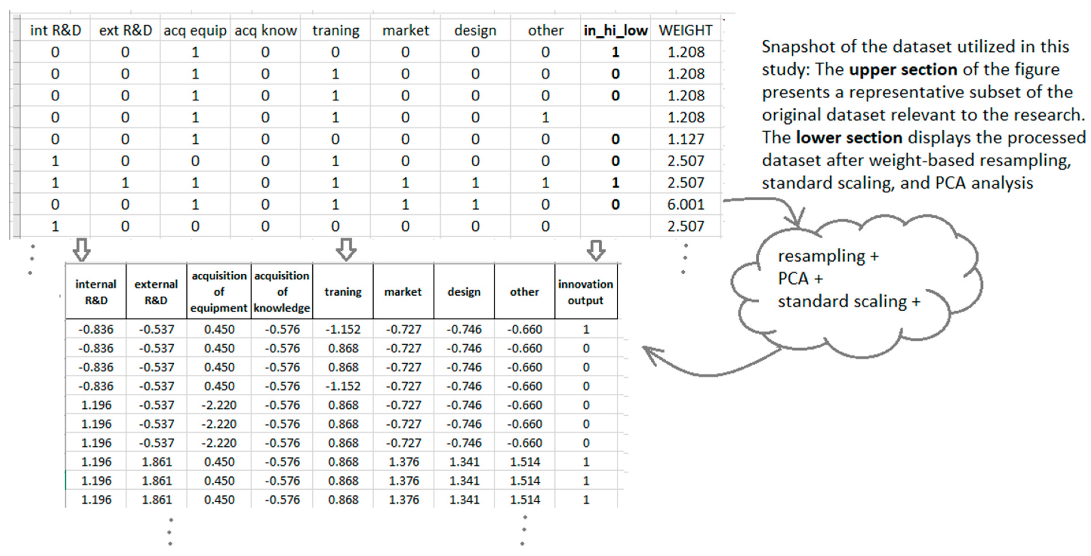
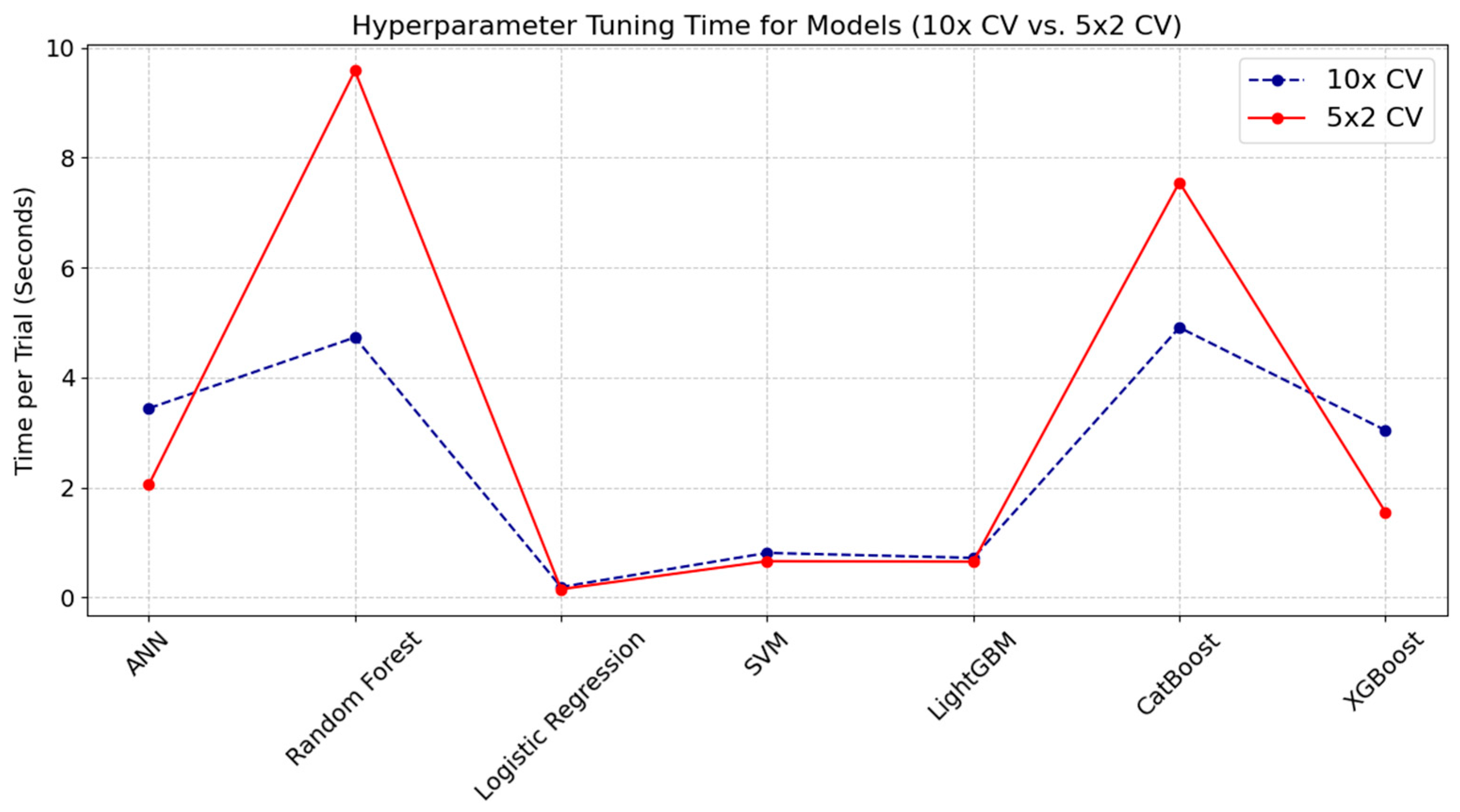
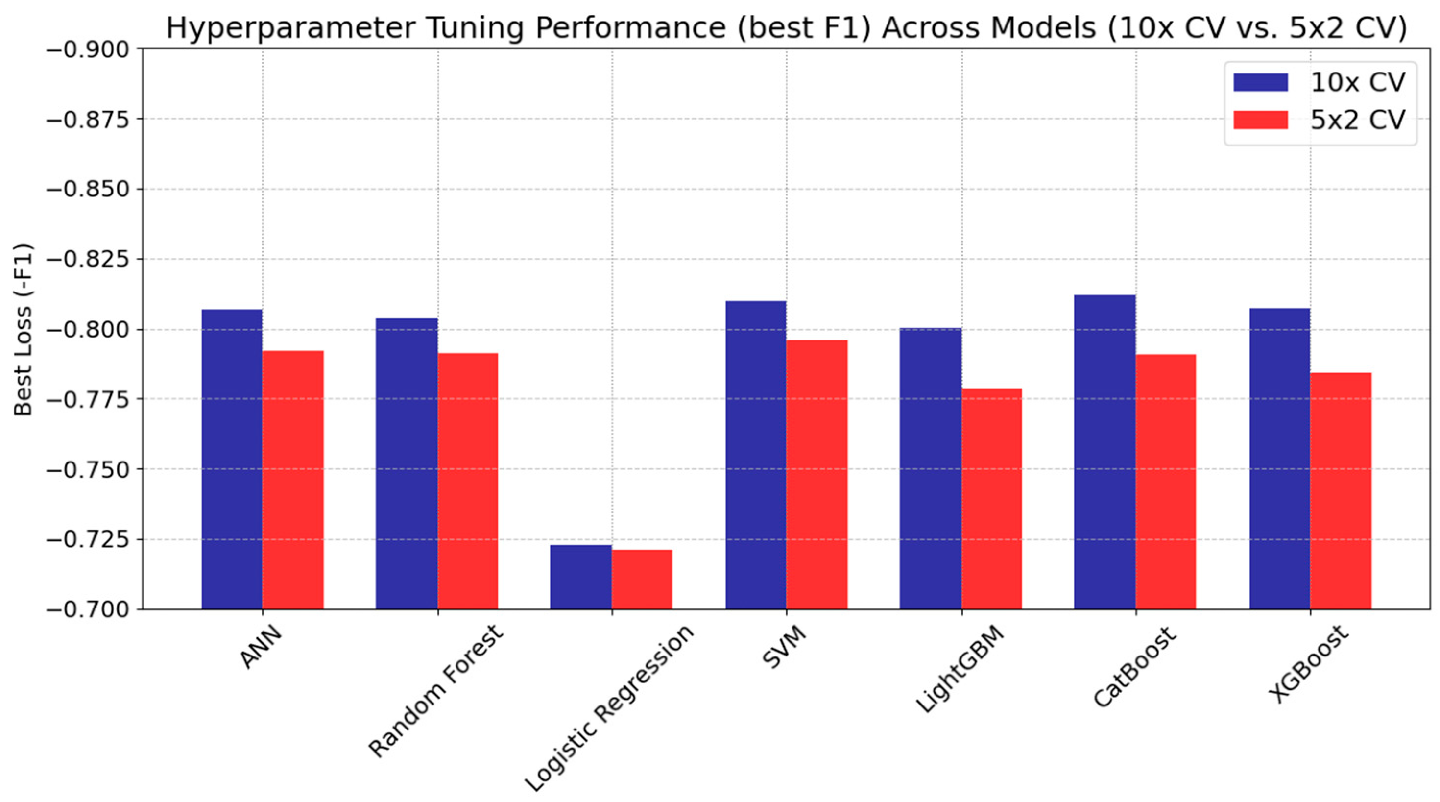
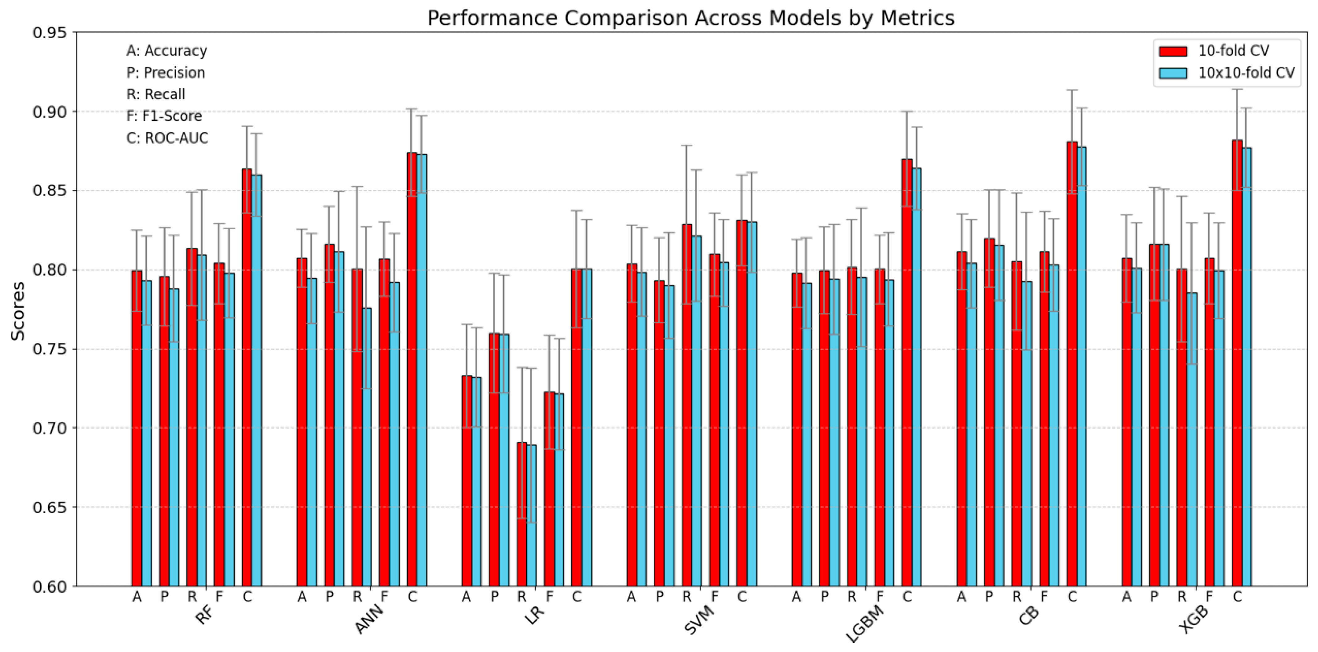
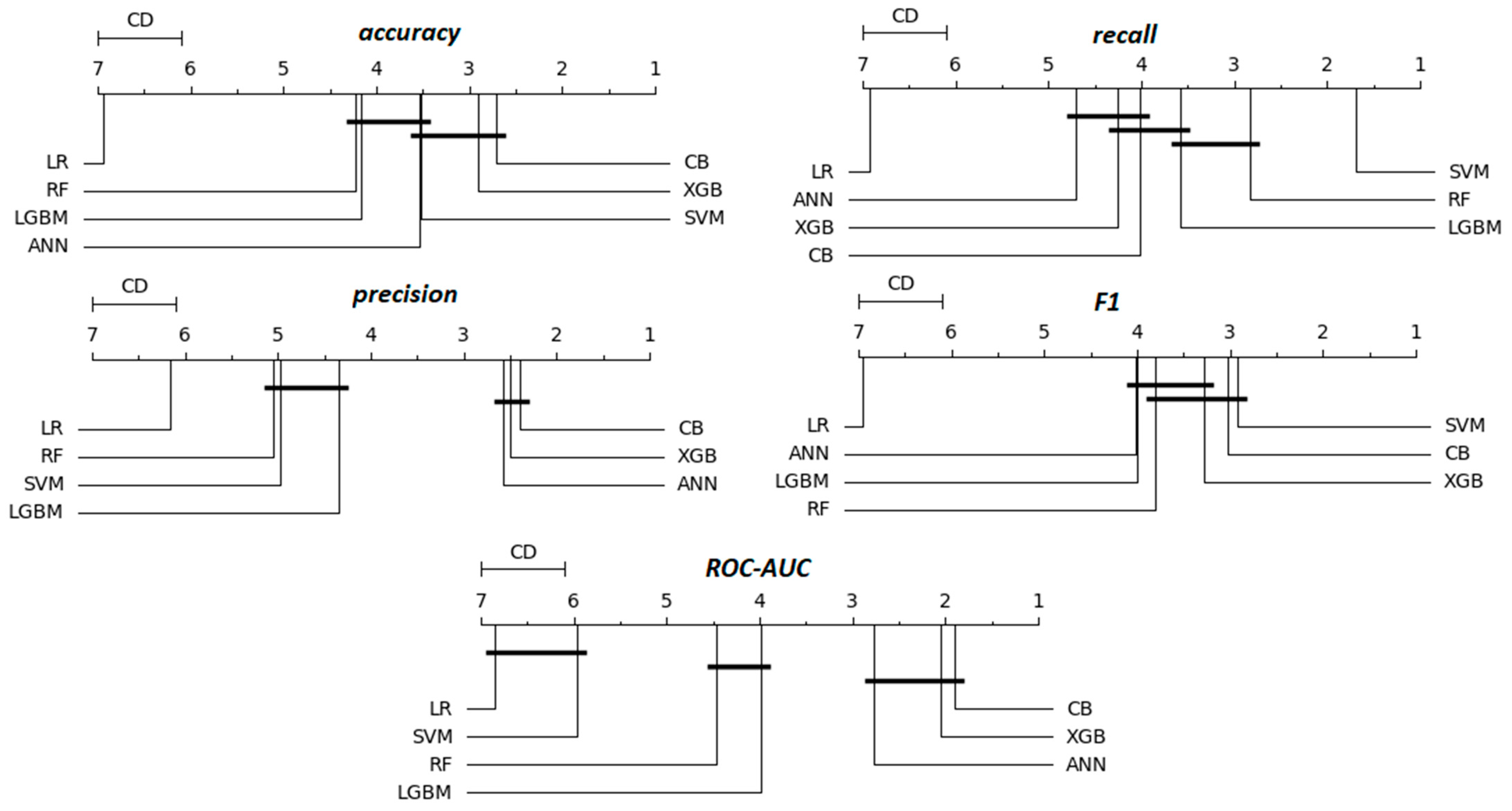
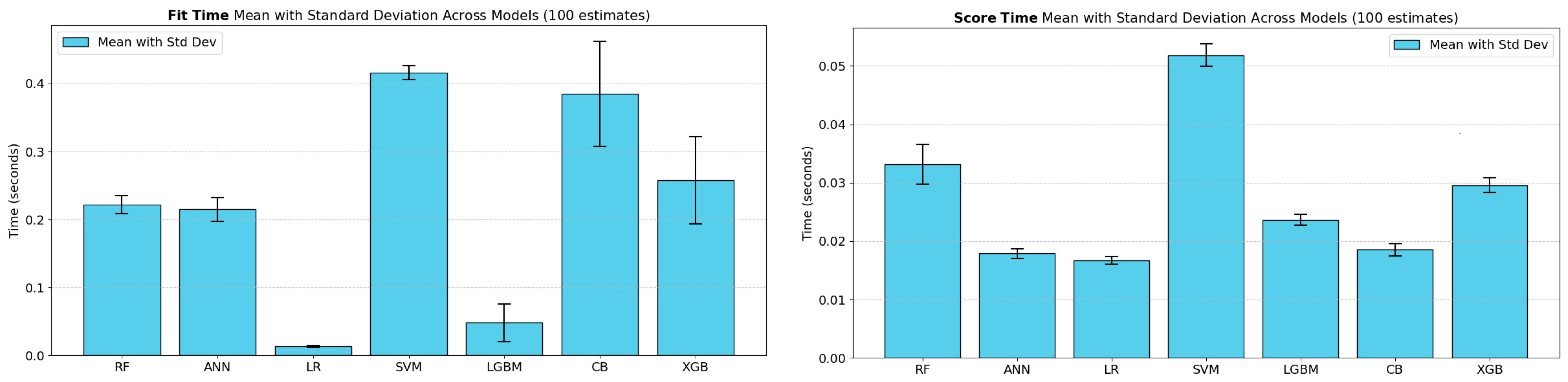
Disclaimer/Publisher’s Note: The statements, opinions and data contained in all publications are solely those of the individual author(s) and contributor(s) and not of MDPI and/or the editor(s). MDPI and/or the editor(s) disclaim responsibility for any injury to people or property resulting from any ideas, methods, instructions or products referred to in the content. |
© 2025 by the authors. Licensee MDPI, Basel, Switzerland. This article is an open access article distributed under the terms and conditions of the Creative Commons Attribution (CC BY) license (https://creativecommons.org/licenses/by/4.0/).