Abstract
Persistent atrial fibrillation (AF), a prevalent cardiac arrhythmia, is primarily sustained by rotor-type reentries, with their localization crucial for successful ablation treatment. Fractionated atrial electrogram (EGM) signals have been associated with the tips of the rotors and are thus considered as ablation targets. However, the typical noise problems of physiological signals affect the results of EGM processing tools, and consequently the ablation outcome. This study proposes a data fusion framework based on the Joint Directors of Laboratories model with six levels and information quality (IQ) assessment for locating rotor tips from EGMs simulated in a two-dimensional model of human atrial tissue under AF conditions. Validation tests were conducted using a set of 13 IQ criteria and their corresponding metrics. First, EGMs were contaminated with different types of noise and artifacts (power-line interference, spikes, loss of samples, and loss of resolution) to assess tolerance. The signals were then preprocessed, and five statistical features (sample entropy, approximate entropy, Shannon entropy, mean amplitude, and standard deviation) were extracted to generate rotor location maps using a wavelet fusion technique. Fuzzy inference was applied for situation and risk assessment, followed by IQ mapping using a support vector machine by level. Finally, the IQ criteria were optimized through a particle swarm optimization algorithm. The proposed framework outperformed existing EGM-based rotor detection methods, demonstrating superior functionality and performance compared to existing EGM-based rotor detection methods. It achieved an accuracy of approximately 90%, with improvements of up to 10% through tuning and adjustments based on IQ variables, aligned with higher-level system requirements. The novelty of this approach lies in evaluating the IQ across signal-processing stages and optimizing it through data fusion to enhance rotor tip position estimation. This advancement could help specialists make more informed decisions in EGM acquisition and treatment application.
1. Introduction
Atrial fibrillation (AF) is one of the most common cardiac pathologies worldwide, with an estimated prevalence of 1.5–2% [1]. Catheter ablation has emerged as a widely used therapeutic alternative to pharmacological management, particularly in cases where medical treatment has proven ineffective [2]. While pulmonary vein isolation has demonstrated efficacy in treating paroxysmal AF, its success rate remains limited in persistent AF cases [3]. This discrepancy has increased interest in identifying the specific localization of the arrhythmogenic sources that sustain AF [4]. One proposed mechanism involves rotors, which are spiral waves that revolve around a singular point known as the rotor tip. These structures have been hypothesized as key drivers of AF, continuously reactivating atrial tissue and sustaining the arrhythmia [5]. According to the rotor hypothesis, AF is maintained by one or several rotor-type functional reentries, making them key targets for ablation. Therefore, identifying and localizing rotor sites is crucial, as ablation targeting them has been proposed to disrupt AF-sustaining mechanisms and improve treatment outcomes. Clinical evidence supports the pivotal role that rotors play in the persistence of AF [6,7,8].
Despite the significance of rotors, their precise locations remain undetermined. Electrophysiological procedures attempt to detect rotor positions by analyzing atrial electrical activity through catheter recordings known as electrograms (EGMs). Consequently, AF treatment strategies based on rotor ablation rely on the accurate identification of rotor tips by EGM processing. Numerous studies have explored the identification of ablation zones by analyzing EGMs, yet this remains an open area of research. Some studies have linked the occurrence of complex fractionated atrial electrograms (CFAEs) with the rotor tip [9,10,11], suggesting that these signals could serve as potential ablation landmarks for persistent AF treatment [12,13,14]. However, this process requires multiple simultaneous recordings across the atria, exposing the signals to significant noise and artifacts. Various techniques have been proposed for EGM processing to determine ablation zones, including dominant frequency (DF), approximate entropy (ApEn), sample entropy (SampEn), and time-frequency characteristics [10,15,16,17]. While these approaches perform well under controlled conditions with minimal disturbances, their effectiveness diminishes in real-world scenarios due to noise and artifacts in recorded EGMs [4,18,19,20]. Common sources of noise and artifacts in physiological signals include high-frequency interference, power grid noise, motion artifacts, and electrode contact loss. Although signal processing techniques exist to mitigate these disturbances, they may alter relevant information about the underlying arrhythmogenic mechanisms, potentially affecting the accuracy of rotor localization [21,22,23,24,25,26]. In clinical settings, careful consideration must be given to noise sources and artifacts when designing signal processing tools. Despite advancements in filtering and noise reduction, preprocessing steps can still impact the quality of extracted quantitative information. Achieving an optimal balance between noise suppression and information preservation remains a critical challenge for reliable rotor detection based on EGMs. Studies have assessed the influence of noise on EGM characterization using entropy estimators, considering various contamination sources such as signal saturation, poor electrode contact, and far-field activity. The findings indicate that selectively eliminating low-fidelity EGMs significantly enhances the density and stability of rotor tip detection [20].
Computational approaches have been developed to address these challenges and improve real-world applicability. However, denoising and artifact suppression inevitably affect signal quality, potentially altering extracted quantitative features such as frequency content, entropy, and energy. To the best of our knowledge, no studies have comprehensively analyzed the combined effects of multiple noise sources and the robustness of feature extraction techniques used for ablation zone detection while incorporating information quality (IQ) assessments at different stages of EGM processing. In this context, data fusion techniques provide a powerful framework to enhance signal interpretation and robustness. The Joint Directors of Laboratories (JDL) model, the most widely adopted framework for data fusion, provides a structured methodology integrating statistical and computational techniques across multiple processing levels to enhance situational understanding. Initially proposed with four levels in [27], the model was later expanded to six levels in [28]. As illustrated in Figure 1, the JDL model operates through a data bus connecting these six processing levels. The JDL model organizes data fusion into six hierarchical levels, where the lower levels (0 and 1) process numerical data to determine object position, kinematics, and identity, while the higher levels (2 and 3) interpret context for decision-making, using symbolic and probabilistic techniques such as logic, evidence theory, and neural networks [29]. Specifically, level 0 (preprocessing) prepares raw data through noise reduction, calibration, and alignment using methods like Kalman filtering and Fourier transforms. Level 1 (object refinement) identifies and tracks objects, updating their states through classification, tracking, and data association. Level 2 (situation refinement) analyzes interactions and behaviors by integrating spatial and temporal information, employing Bayesian networks and Markov logic networks. Level 3 (impact/risk refinement) assesses potential outcomes and risks using predictive models such as hidden Markov models and dynamic Bayesian networks. Level 4 (process refinement) optimizes resource allocation and system adjustments through adaptive filtering and optimization techniques, ensuring continuous evaluation of the data fusion process. Finally, level 5 (user refinement) supports decision-making by effectively presenting fused data using decision theory and user modeling. This structured approach enhances situational awareness and facilitates informed decision-making across various applications. This model has been applied in bioinformatics, infrastructure, and other domains [30,31,32,33].
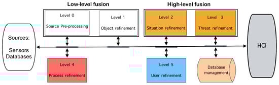
Figure 1.
Joint Directors of Laboratories (JDL) fusion model. HCI: Human-computer interaction.
This work proposes a data fusion framework based on the JDL functional model [34] and IQ assessment for rotor localization in persistent AF. Our approach utilizes simulated EGMs in a two-dimensional (2D) atrial tissue model. Our main contributions are the following: (i) Integrating a multi-level data fusion approach to enhance rotor tip estimation. (ii) The incorporation of an IQ-driven optimization process to improve signal processing robustness against noise and artifacts. (iii) The validation of the proposed framework through extensive simulations under different perturbation scenarios. This novel approach aims to support clinical decision-making by providing more accurate and reliable rotor localization for ablation therapy.
2. Materials and Methods
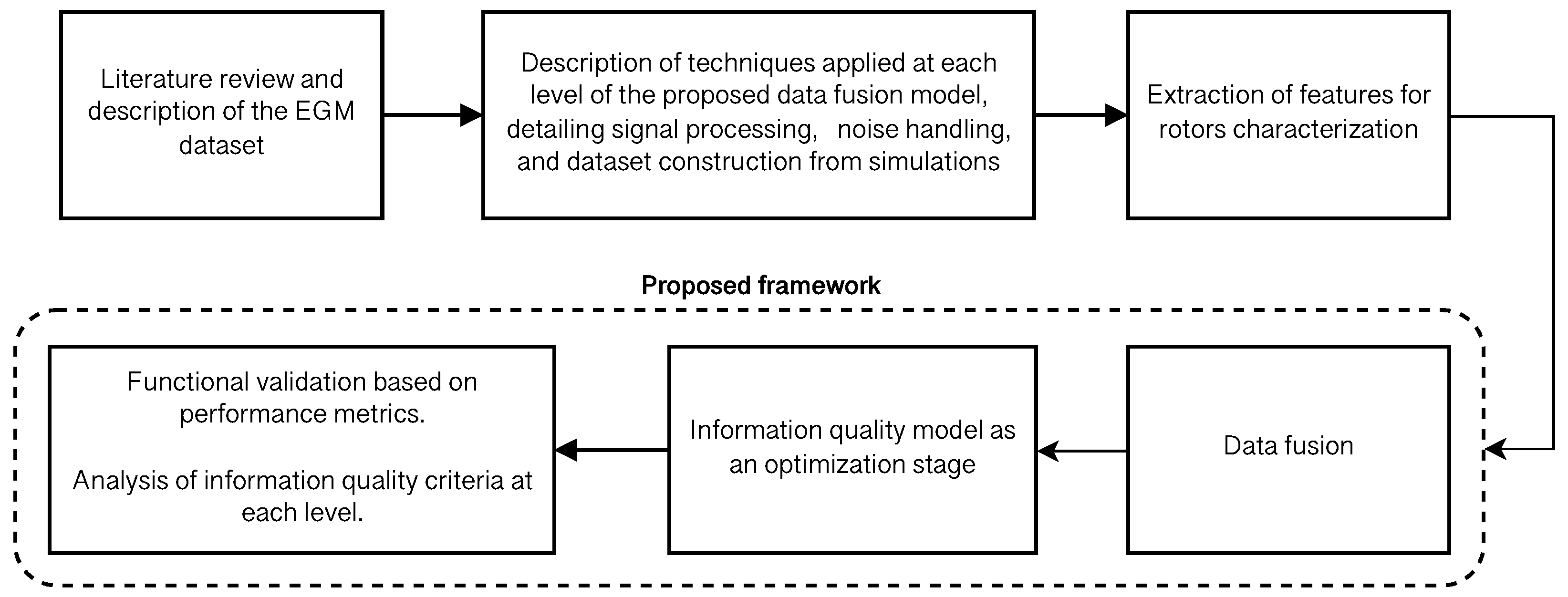
Figure 2 outlines the overall methodological design. The high-level methodology used in this study includes stages for literature review and data description, technique analysis, feature extraction, data fusion, quality information modeling, and functional validation.
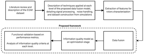
Figure 2.
Flowchart illustrating the building blocks of the methodological sequence of the study and the integration of different phases in the development of the data fusion model.
2.1. Rotor in a 2D Model of Human Atrial Tissue Under Atrial Fibrillation Conditions
A 2D model of human atrial tissue was designed as a 6 × 6 cm2 surface, discretized into 150 × 150 grid points with a spatial resolution of 400 m. The cellular electrophysiology was simulated using the Courtemanche human atrial action potential model [35]. To reproduce the electrical conditions of isolated myocytes from patients with AF [36,37,38], the conductances of different ionic channels were adjusted as follows: the maximum conductances of the ultra-rapid outward potassium current and the L-type calcium current were both reduced by 35%, the maximum conductance of the ultra-rapid outward potassium current was reduced by 50%, and the maximum conductance of the inward rectifier potassium current was increased by 100%. These conductance adjustments aimed to simulate AF-induced electrical remodeling. Additionally, the cholinergic effect was simulated by incorporating the acetylcholine-dependent potassium current with an acetylcholine concentration of 5 nM.
The atrial cell model was integrated into the 2D virtual tissue. In a previous work [17], the action potential propagation over a 2D domain was modeled using a fractional diffusion equation. Isotropy and standard diffusion conditions were simulated to obtain a real conduction velocity of 67 cm/s. Discretization and the numerical solution of the propagation equation were accomplished using a semi-spectral approach previously reported [39], using a time step of 0.01 ms.
A rotor propagating pattern was generated by applying the S1–S2 cross-field stimulation protocol. S1 is a train of stimuli applied to the left border of the tissue, a region containing nodes. Once the wave generated by the last S1 stimulus had passed the middle of the domain, a single S2 extra stimulus was applied to the first quarter of the domain (75 × 75 nodes), generating a single rotor (Figure 3). Each stimulus consisted of a rectangular pulse lasting 2 ms with a current of 4200 pA.

Figure 3.
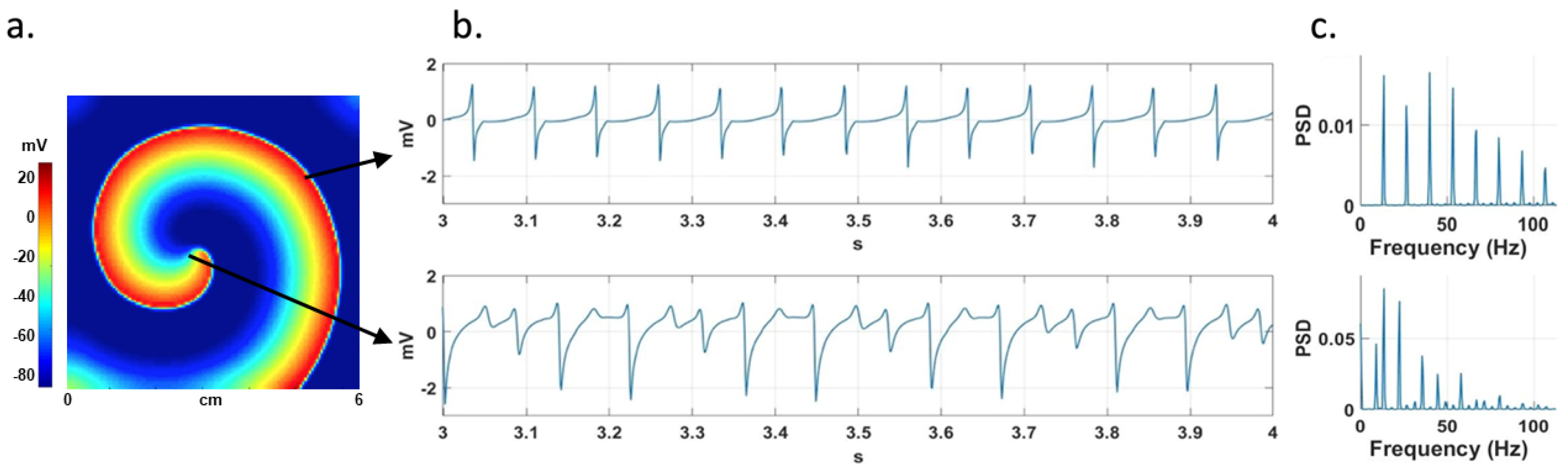
(a) Stable rotor in a 2D atrial model. The arrows indicate the points where two EGMs are recorded, one at the rotor tip and the other far from it. (b) Non-CFAE (top) and CFAE (bottom) signals, and (c) their corresponding PSDs.
2.2. Electrograms
The numerical solution of the AF electrophysiological model provides the transmembrane potentials at specific grid points within the atrial tissue, which are then used to compute EGM signals. Unipolar EGMs are modeled as the extracellular potential measured by a positive polarity electrode whose reference (zero potential) is at infinity. The extracellular potential () was calculated using the large-volume conductor approximation [40], as described by the following equation:
where K is a constant representing the ratio of intracellular to extracellular conductivity. The extracellular potential is computed at the measurement point r. This potential depends on the configuration of the transmembrane potential across the tissue. The source points contribute to the measured potential at r. The nabla operator is the gradient that is being taken with respect to the source coordinates . This is necessary because the potential is being integrated over the source points , while r represents the position of the measurement point. is the distance from the source (x, y, z) to the measurement point (, , ), and is the volume differential. A total of 22,500 virtual electrodes (150 × 150), spaced by 0.4 mm, were used to calculate the EGM signals (one for each node of the model).
In this study, CFAEs were defined as irregular signals exhibiting multiple (>2) positive or negative deflections with varying amplitudes [41]. Non-CFAEs were defined as signals with single and regular deflections. The power spectral density (PSD) of the signals was estimated using the fast Fourier transform. Figure 3a shows a stable simulated rotor. Figure 3b shows a non-CFAE signal from a region far from the rotor tip and a CFAE signal from the rotor tip area, while Figure 3c presents their corresponding PSDs.
2.3. Noise
The EGMs obtained from the simulations are combined with different types of noise and artifacts that modify their frequency spectrum, namely, power line interface, spikes, loss of samples, and loss of resolution, as described below.
2.3.1. Power Line Interference (PLI)
The harmonics of the electrical power line, typically at frequencies of 50 Hz or 60 Hz, are a significant source of contamination for electrophysiological signals. The nominal power supply is 230 V/50 Hz or 120 V/60 Hz, with fluctuations of 10% in voltage and 1% in frequency. However, it often contains harmonics and interharmonics, albeit with limited relative power content. PLI affects many physiological recordings, including bipolar and unipolar EGMs, often exhibiting amplitude and frequency variations, as well as harmonic content beyond the limits established by its bandwidth. In this study, these characteristics of PLI are considered to adequately approximate the real effects of these perturbations. Random variations within the intervals mentioned above were applied to the amplitude and frequency of the main 60 Hz component, as well as to its first four harmonics. The components were also frequency-modulated with a maximum deviation of 0.5 Hz to introduce low-amplitude interharmonics. The resulting signal, referred to as common PLI, was used to obtain noisy EGM recordings with signal-to-interference ratios (SIRs) of 25, 20, 15, 10, and 5 dB.
2.3.2. Spikes
Spikes are transient impulses that occur during signal acquisition due to sensor failures, loss of contact, or movement. Spikes are defined as sharp pulses with rising and falling linear edges. They are a relatively frequent interference in biomedical signals. They may be due to sensor failures, amplifier saturation, patient movement, external interference, pacemakers, or processing errors [42]. A train of spikes is defined by a random process , where represents the percentage of spikes occurring in a series of length N. The amplitude of the spikes is defined as a uniform random variable (, ), where is the maximum peak-to-peak amplitude of the original EGM. Mathematically, is defined as
where is the amplitude of the spike obtained from , denotes the Dirac delta centered at the time instant , and the values of are generated by process .
2.3.3. Loss of Samples and Loss of Resolution
These issues are caused by failures in the acquisition system, including poor electrode contact, electrode displacement, and power supply noise. In a previous study [20], EGMs obtained during clinical procedures revealed that between 5% and 10% of the recordings may exhibit low quality due to three potential noise sources: (i) non-viable data due to saturation of signal, (ii) reduced quality due to poor contact of the electrodes, and (iii) deflections due to far-field activity. These types of noise cause data saturation, which occurs when EGM samples or entire EGM signals are randomly removed, known as loss of samples and loss of resolution, respectively. In the case of loss of samples, the number of discarded samples is set as a percentage of the total number of samples N in the EGM signal. In the case of loss of resolution, data completeness is affected by the loss proportion , where M represents the total number of virtual EGM signals.
2.3.4. Noise Addition to EGMs
First, spike perturbations were added to the EGM signals, using 15 realizations of random spike trains, each with a pulse width of a single sample and probabilities of . The methodology presented in [4] was adopted to generate five databases of EGMs for each value of . A 60 Hz PLI was added to the original EGMs, with frequency fluctuations of [±1%, ±5%] and signal-to-noise ratios (SNRs) of [−5, 0, 5, 10, 15] dB. The methodology of [19] was implemented to generate five databases of EGMs for each value of SNR. Finally, five datasets containing EGMs with loss of samples were generated by adopting , and for the loss of resolution perturbation. Five EGM datasets were generated using the following test values: . Figure 4 depicts examples of each type of noise.
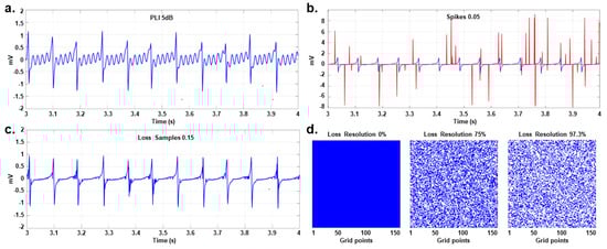
Figure 4.
Examples of different types of noise. (a) One-second view of an EGM with PLI at 5 dB. (b) Spike train (red line) generated on a regular EGM (blue line) with . (c) EGM with loss of samples at 0.15. (d) Losses of resolution of 0%, 75%, and 97.3%, where the blank spaces indicate lost signals.
Table 1 summarizes the configuration of each perturbation applied to the EGMs. The methodology of [4] was considered to generate the perturbed EGMs databases. Furthermore, twelve additional perturbed EGM databases were created by combining different types of noise and considering the variability generated in different feature types to evaluate the proposed framework under various scenarios.

Table 1.
Configuration of EGM perturbations for each validation database.
2.3.5. Noise Tolerance of the Features
The generated datasets were used to test the tolerance of the features to different types of noise at different levels. The noise tolerance of the statistical features—namely, ApEn, SampEn, ShEn, mean, and STD—in detecting the rotor tip was assessed against the different types of noise. The results were compared in relation to the location of the rotor tip obtained from noise-free signals. Accuracy was evaluated in terms of Euclidean distance, and visual sharpness was assessed by a user. Following the procedure presented in [4], the ability to discriminate between CFAE and non-CFAE signals was analyzed using a Mann–Whitney U test with p-values of [0.001, 0.05, 0.01] applied on EGMs. The Euclidean distance was calculated to determine the location of the rotor tip. Similar procedures were applied to the remaining level 1 metrics presented in Table 2.
Table 2.
Definitions of information quality criteria and metrics by level.
2.4. Statistical Features
The statistical features, including the mean, standard deviation (STD), and three distinct entropy measures, are calculated for each EGM signal. Entropy quantifies the average amount of information transmitted during a given process and has been extensively studied for EGM characterization. ApEn and SampEn are commonly applied to processing EGMs. These entropy metrics depend on three parameters, denoted as m, r, and N, where N is the length of the time series, m is the length of the sequences to be compared, and r is the tolerance for accepting coincidences among sequences [43,44].
2.4.1. Approximate and Sample Entropy
ApEn(m, r, N) can be applied to short and noisy time series of clinical data [43]. Series with more frequent and similar sequences lead to lower ApEn values. The ApEn is calculated using the following expression:
The tuning of the parameters m, r, and N is explained in [43], and the function is defined as follows:
where represents the number of sequences that are close to the i-th sequence of length m. The closeness is determined by the parameter r. In practice, the ApEn has two major drawbacks. First, the estimation of the ApEn is affected by the length of the signal, and tends to be uniformly lower than the theoretical value for short recordings. Second, it lacks relative consistency. To address these limitations, the authors of [44] proposed the SampEn.
SampEn(m, r, N) is the negative natural logarithm of the conditional probability that, given two similar m-sample sequences, they remain similar for samples [44]. Therefore, a low SampEn value indicates higher regularity in the time series. The definition of SampEn is as follows:
where and are defined as follows:
where is the number of times the sequence , , is close to according to threshold r; is similar to but considers sequences of length . The tuning of the parameters r, m, and N is the same as for ApEn [44].
In this study, the ApEn and SampEn values are calculated using and , where is the STD of the signal, consistent with prior research [43,44]. The parameter r acts as a threshold that determines the closeness between all pairs of segments of length m within the signal. To estimate ApEn or SampEn, this closeness assessment is also performed for all segments of length . By setting r, the number of segments that are similar to a given segment of m samples are counted, and the probability of similar segments within the signal is subsequently calculated. Then, the resulting estimates of ApEn and SampEn are independent of the amplitude of the signal.
2.4.2. Shannon Entropy
Shannon entropy (ShEn) is a statistical measure of signal complexity. It was estimated by computing the signal histogram using a bin size 0.01 times the signal range, with its value expressed in absolute terms (mV). This histogram configuration has been used in previous studies of atrial fibrillation electrograms [17]. It is mathematically defined as follows:
where is the probability of occurrence of the i-th interval of values in a given signal, and N is the number of possible amplitude values. If a specific amplitude value occurs in 100% of the samples, indicating complete predictability, the ShEn value will be 0. If all amplitude values have an equal chance of occurring, the entropy value will be 1.
2.4.3. Statistical Measurement Maps
A database of 22,500 EGMs, each 5 s long, was obtained from AF episodes simulated in the 2D tissue model. The EGMs contain single (non-CFAE), double, and CFAE potentials.
Figure 5 depicts the 2D maps of atrial tissue representing the five statistical features adopted in this work. For each EGM signal, a single statistical value is calculated, and the map is built using the estimated statistical values for each EGM from the AF simulation, as follows: SampEn and ApEn with parameters and in agreement with previous works [43,44], and , matching the EGM signal length. In addition, the mean, STD, and ShEn are computed. These calculations are based on the last 4 s of the EGM signals, as the first second is discarded to exclude the transient phase associated with the stabilization phase of the fibrillatory conduction pattern.
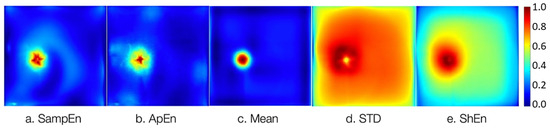
Figure 5.
Maps of the statistical features computed from the 22,500 noise-free EGMs correspond to a rotor simulation in the 2D atrial model. (a) SampEn, (b) ApEn, (c) mean, (d) STD, and (e) ShEn. The color scale depicts the normalized values of statistical estimates.
2.5. Proposed JDL-Based Framework
Figure 6 illustrates the proposed JDL-based framework, which was originally expanded to six levels by [28] and adapted for identifying and evaluating potential ablation zones using EGMs derived from rotor simulations under AF conditions.
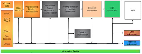
Figure 6.
Proposed JDL-based framework adapted to determine the ablation zone (rotor tip) using EGMs. The six levels of the JDL model are specified. HCI stands for human-computer interaction.
The levels of the JDL model are specified as follows:
- (i)
- Level 0: The EGM signals are normalized to the interval [−1, 1], and wavelet filtering is performed to eliminate the PLI noise. Spikes and lost samples are identified, and these samples are approximated using the inverse distance-weighted algorithm, considering the spatially closest signals. Missing signals are approximated using the same algorithm by considering all known EGMs.
- (ii)
- Level 1: The association, extraction, and selection of EGM features are carried out. The resulting features are used to generate maps of the tissue, aiming to pinpoint the rotor location. Signal fusion is achieved using particle filters to obtain a signal with reduced uncertainty due to noise. This step should be implemented when multiple signals of the same target are available. Feature extraction is performed using the ApEn, SampEn, ShEn, mean, and STD to construct the maps. The resulting maps are merged using the wavelet fusion technique, applied to a pair of images selected based on IQ maximization through an optimization process. In this work, the particle swarm optimization (PSO) algorithm was adopted due to its demonstrated generality and effectiveness in non-linear optimization problems [45].
- (iii)
- Level 2 and level 3: Expert knowledge is expected to be emulated through the processes at these levels, such as case-based reasoning or fuzzy inference systems. The outcomes aim to assess situations, risks, vulnerabilities, and opportunities by considering the information on the rotor tip location and the IQ.Level 2: The situation is assessed based on the IQ of the merged map, considering the rotor tip location as a target. Several fuzzy inference systems (FISs) were designed to analyze the effect of different IQ levels due to the erroneous reasoning of the experts represented in this model. The determination of the rotor tip location is guided by expert-established rules based on experience, which is implemented in a FIS. This system correlates information gathered from previous levels and IQ assessments to identify specific situations. In this work, we propose n situations based on the available information and the IQ, as follows:where , , and refer to the accuracy, precision, and interpretability of the merged maps, respectively. Accuracy is the proportion of correct predictions made by a model relative to the total number of predictions. Precision measures how accurately the model identifies the positive class, i.e., the proportion of the positive predictions belongs to the positive class. Interpretability refers to the extent to which users or researchers can understand and explain the decisions or predictions of the model. , , and correspond to the output fuzzy sets. corresponds to the output fuzzy sets.Level 3: At this stage, the same procedure is adopted as in level 2, but it is applied to risk/impact assessment.
- (iv)
- Level 4: In addition to incorporating expert knowledge, IQ assessment is used to adjust the model throughout the entire processing chain. For this task, an optimization process is performed using the PSO algorithm on IQ models built using support vector regression techniques.
- (v)
- Level 5: Adjustments and fine-tuning of the process are applied based on the knowledge and experience of the user. Such knowledge is used to update, quarantine, or include new cases through a case-based reasoner.
2.5.1. IQ Criteria
We propose a set of IQ criteria based on level fusion. This proposal relies on the functionality of each level and the refinement process in this case study (i.e., EGM processing). Each level is characterized using predictors that relate to the IQ criteria of input and output. A predictor is modeled for each level, and IQ criteria values are collected to measure the IQ in the inputs and outputs of each level. This process is initiated by applying different levels of noise to the EGM databases. In this work, the support vector regression (SVR) technique was used to build the models because this technique has demonstrated high performance in prediction without high data volumes [46].
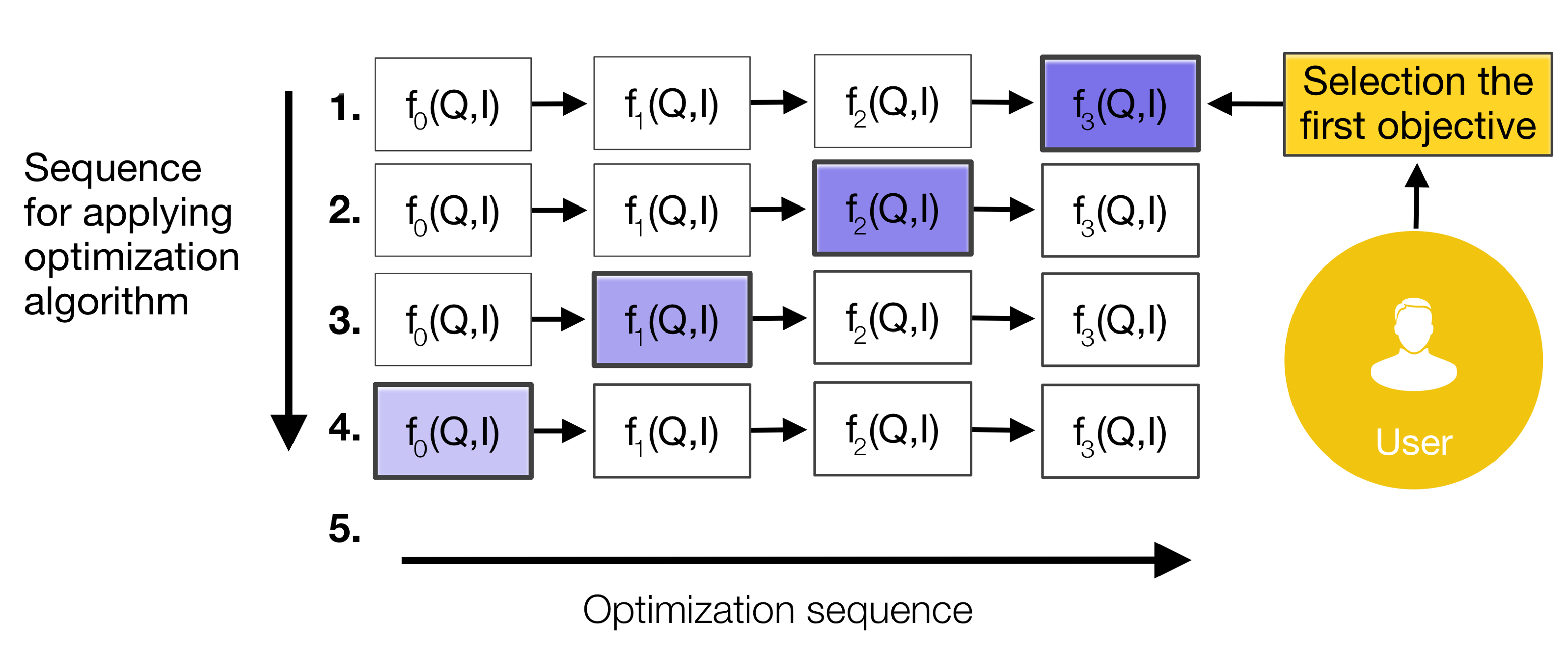
Figure 7 shows the optimization process using the IQ models. The optimization process is carried out considering the results provided by each IQ function and taking into account user requirements. The optimization process is applied at the last level to identify which IQ criteria must be improved in the inputs. This process continues until level 0, after which the refinement process is applied from level 0 to the last level.
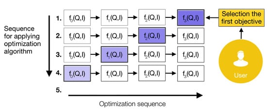
Figure 7.
Optimization process using the IQ models.
Table 2 shows the IQ criteria and the corresponding metrics for each level of the proposed framework. The criteria at level 0 focus on the signals analyzed as a time series. The criteria at level 1 focus on maps (i.e., rotor tip location and its visualization). The reputation criterion is a more complex IQ metric and is quantified by establishing the noise tolerance of the features. This is calculated using the difference between contaminated maps and the ground truth (noise-free maps), where n noisy maps are considered.
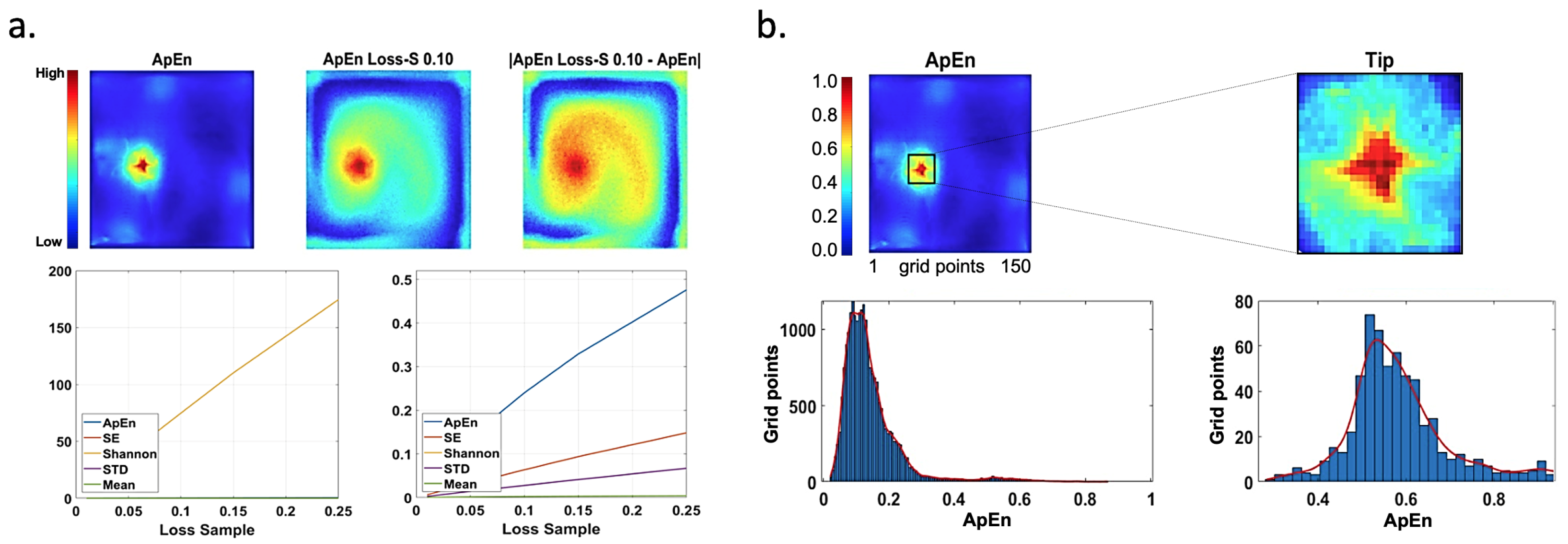
Figure 8a shows the ApEn map without noise and the ApEn with a loss of 10%, and the difference between them (their mean value is 0.2398). In addition, cumulative curves generated by our measurement are portrayed. The ShEn curve is shown in the figure on the left. Another complex IQ criterion is interpretability; it uses the contrast of the rotor tip relative to the rest of the image, considering mean values and low values. This measure was computed from the maps normalized to the interval . Figure 8b shows the ApEn and the extraction of the rotor tip together with histograms of the data, where the red line represents the fit of the data to a normal distribution. The remaining IQ criteria are self-explained through their corresponding metrics listed in Table 2.
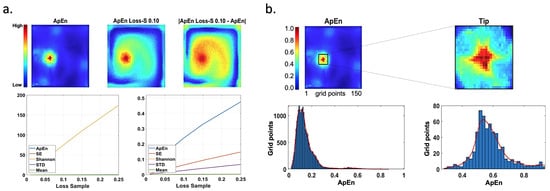
Figure 8.
Reputation and interpretability examples. (a) Noise-free maps of ApEn, with a loss of 10%, and the difference between them (top). Cumulative curves for our measurements versus different values of lost samples for different maps are shown at the bottom, with the ShEn curve displayed on the left. The values of statistics estimations are not normalized. (b) ApEn map and the extraction of rotor tip (top), and their interpretability (bottom) calculated based on the histogram (). The red color line corresponds to data fitted to a normal distribution. The color scale depicts the normalized values of statistics estimations.
2.5.2. Validation
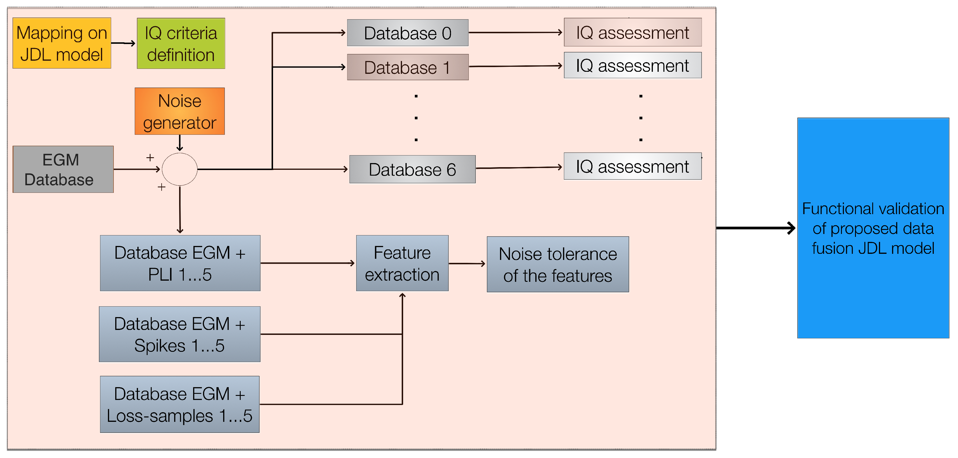
To summarize the methodology, statistical feature maps were computed from the EGM database, which was obtained from a simulated AF episode in the 2D atrial tissue model. A general mapping of the proposed framework was then conducted, followed by the selection of IQ techniques and criteria (along with their corresponding metrics) for each framework level. Subsequently, databases were constructed to validate the proposed framework, with the simulated datasets being affected independently and jointly by various perturbations. The validation process was carried out using the set of databases, as illustrated in Figure 9. The simulated databases were subjected to the following perturbations: (i) PLI, (ii) spikes, (iii) loss of samples, and (iv) loss of resolution. Then, the set of quality metrics was applied to the EGMs with added noise. The complete algorithm, executed on a Mac computer with an M1 Max processor and 64 GB of RAM, requires approximately 3 h to run.
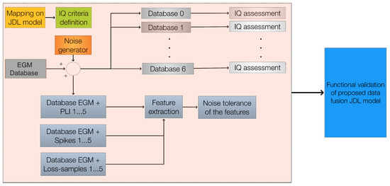
Figure 9.
Experimental procedure before testing the proposed model: a general mapping of the proposed framework is performed; then, techniques and IQ criteria (with their metrics) are selected for each level. Finally, databases are constructed to validate the proposed framework.
3. Results
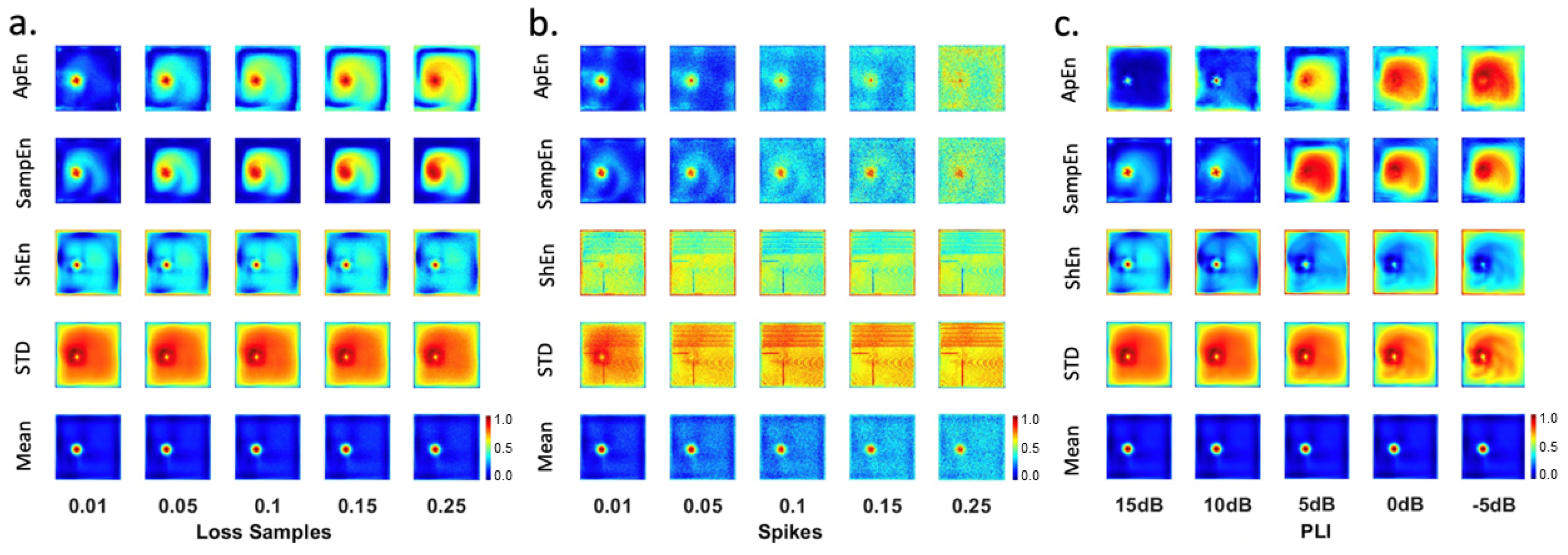
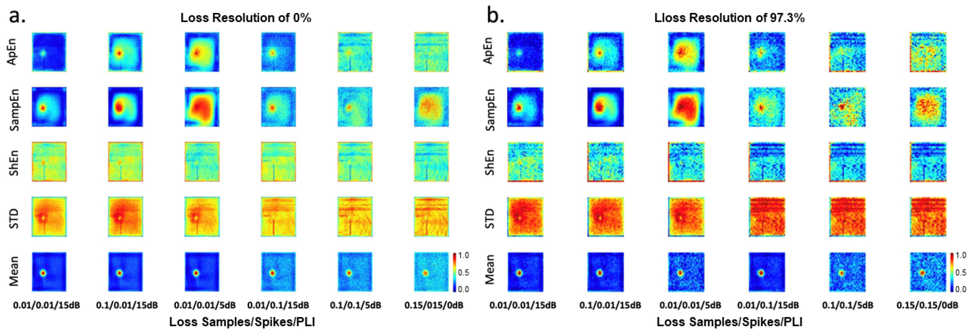
Figure 10 shows the maps generated from the EGMs and affected by the loss of samples (Figure 10a), spikes (Figure 10b), and PLI (Figure 10c). Figure 11a depicts maps affected by different configurations of simultaneous perturbations, including loss of samples, spikes, and PLI. Figure 11b presents the maps with a loss of resolution of 97.3% and affected by different levels of loss of samples, spikes, and PLI. These maps were analyzed by EGM experts to establish the best maps (features least affected by noise) to identify ablation areas.

Figure 10.
Statistical feature maps affected by different levels of perturbations. (a) Loss of samples, (b) spikes, and (c) PLI. The color scale depicts the normalized values of statistics estimations.
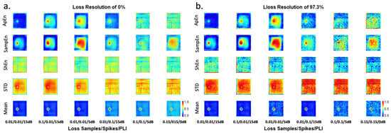
Figure 11.
Statistical feature maps affected by different levels of perturbations of loss of samples/spikes/PLI, with (a) loss of resolution of 0%, and (b) loss of resolution of 97.3%. The color scale depicts the normalized values of statistics estimations.
The analysis is detailed below.
- (i)
- EGM maps affected by the loss of samples: Mean maps reveal the rotor tip area. The rest of the tissue has low values, demonstrating regular activity. A similar performance was observed for the ApEn map with a loss of samples and the SampEn map with a loss of samples . The ApEn and SampEn maps show a high-value area where the rotor tip is located. Intermediate values appear in regions of regular activity where low values are expected. In addition, ApEn and SampEn maps present the characteristic star shape corresponding to the slight migration of the rotor. The worst maps are generated by the STD and ShEn features, which exhibit high values at the edges and intermediate values in regions of regular activity.
- (ii)
- EGM maps affected by spikes: The best outcomes are observed for the mean map, followed by the ApEn map, and the SampEn map affected by spikes at , , and . The STD and ShEn maps do not yield good results.
- (iii)
- EGM maps affected by PLI: All mean maps are useful for rotor detection, as they allow the identification of a very specific rotor tip area, while low amplitudes are observed in the rest of the tissue, where regular electrical activity occurs. The first two SampEn maps could be useful, as they reveal the characteristic star shape of the slight migration of the rotor tip. However, intermediate values appear in regions of regular activity, where low values would be expected. The ApEn and ShEn maps exhibit issues with high values at the borders.
- (iv)
- EGM maps simultaneously affected by different configurations of loss of samples, spikes, and PLI (Figure 11): The mean map performs well under the following noise configurations 0.01/0.01/15dB, 0.1/0.01/15dB, and 0.01/0.01/15dB. The remaining mean maps are similar. The SampEn maps with noise configurations of 0.01/0.01/15dB and 0.01/0.1/15dB to allow the identification of the rotor tip. The ApEn maps with noise configurations of 0.01/0.1/15dB and 0.1/0.01/15dB exhibit a reduced area of high amplitudes. The other maps are not suitable for identifying ablation areas.
For each set of noise-contaminated signals (i.e., level 0), the following quality measures were calculated: accuracy—spikes, accuracy—PLI, data—amount, and completeness. The absolute values of the Pearson correlations between pairs of quality criteria from level 0 are presented in Table 3. High correlations are observed between the following pairs: accuracy—spikes and spikes—real, accuracy—PLI and data—amount, and completeness and loss of samples.
Table 3.
Correlation between pairs of IQ criteria at level 0.
Using a significance level of 5% (p-value) to test the null hypothesis of no correlation against the alternative hypothesis of a nonzero correlation, the results indicate no significant evidence of the correlation between the following pairs: data—amount and accuracy—spikes, data—amount and all other criteria, accuracy—PLI and completeness, accuracy—PLI and loss of samples, accuracy—PLI and PLI—real, accuracy—PLI and spikes—real, and accuracy—spikes and loss of samples—real. For the remaining criteria, the results provide significant evidence supporting the absence of correlation.
For level 1, four quality criteria (i.e., consistency, accuracy, precision, and reputation) were calculated from 110 maps (i.e., ApEn, mean, STD, SampEn, ShEn). The metrics applied for each criterion are described in Table 2. The correlations among level 1 quality criteria are listed in Table 4. There are no high correlations among quality criteria, and considering a significance level of to test the null hypothesis of no correlation against the alternative hypothesis of a nonzero correlation, there is no significant evidence of a lack of correlation between reputation and consistency, while there is significant evidence of a lack of correlation for the other criteria.
Table 4.
Correlation between pairs of IQ criteria at level 1.
To determine the effects of IQ among levels, correlations were calculated between IQ inputs and IQ outputs. Table 5 presents the correlations between pairs of IQ inputs (where outputs of level 0 serve as inputs of level 1) and IQ outputs of level 1. There are no high correlations among quality criteria. Considering a significance level of , there is significant evidence of a lack of correlation between consistency and accuracy—PLI, precision and loss of sample, and precision and PLI. For reputation, there is no significant evidence of a lack of correlation between accuracy—spikes and spikes. The accuracy of level 1 shows significant evidence of a lack of correlation with all variables of level 0. Since accuracy shows no correlation, a dependency analysis was performed using the ReliefF algorithm with 11 nearest neighbors [47].
Table 5.
Correlation between pairs of IQ criteria at level 1 (input–output).
Table 6 summarizes the correlations between pairs of IQ inputs (outputs of level 1) and IQ outputs of level 2. Objectivity is highly correlated with interpretability, reputation of input with reputation of output, consistency with objectivity, and reputation of output with accuracy of input. These correlations highlight the most relevant IQ factors affecting data processing. Similarly, Table 7 shows correlations among the IQ inputs (outputs of level 2) and IQ outputs of level 3. There is a high correlation between accuracy and interpretability and between the objectivity of input and output. Efficiency shows no correlations with any IQ criteria except for interpretability at level 2.
Table 6.
Correlation between pairs of IQ criteria at level 2 (input–output).
Table 7.
Correlation between pairs of IQ criteria at level 3 (input–output).
To maximize the quality of the IQ results at each level, support vector regression was applied to model IQ by level, using 80% of the data for cross-validation and 20% for testing. The performance of these models is shown in Table 8, Table 9 and Table 10 in terms of mean absolute error (MAE), mean absolute percentage error (MAPE), and root mean squared error (RMSE). Particle swarm optimization was applied to determine the IQ inputs that maximize the IQ output criteria.
Table 8.
Performance (error) of SVR models of IQ at level 1.
Table 9.
Performance (error) of SVR models of IQ at level 2.
Table 10.
Performance (error) of SVR models of IQ at level 3.
4. Discussion
Clinical evidence indicates that rotors are a key mechanism sustaining AF [6,7,8]. EGM-guided ablation targets arrhythmogenic mechanisms, such as rotors, by detecting the rotor tip through EGM signal processing [12,13,14]. However, this process is challenged by noisy conditions, artifacts, and poor electrode contact, leading to signal distortions such as amplifier saturation spikes and motion artifacts [20,48]. While filtering and noise suppression techniques have advanced, common noise sources, including high-frequency interference, power grid noise, and far-field activity, continue to affect EGM processing accuracy. Prior studies highlight that selectively eliminating low-quality EGMs enhances rotor detection stability and density [20,21]. However, standard preprocessing methods often rely on filter banks, which, despite removing noise, can alter signal integrity and compromise key quantitative features such as frequency content, entropy, and energy [22,23,24,25,26].
Given these challenges, our study proposes a JDL-based framework to evaluate and preserve IQ across different EGM processing stages. Unlike conventional rotor detection strategies, which primarily focus on localizing rotor positions [6,7,8], our approach systematically assesses IQ degradation due to preprocessing and implements a data fusion scheme to retain critical information. Instead of discarding low-IQ signals, our framework integrates multiple data sources to enhance reliability.
Our study also considers the impact of noise and preprocessing strategies on EGM analysis. Some studies exclude preprocessing to assess robustness against noise, while others implement denoising techniques before analysis [4,20]. Significant variability in EGM-based metrics has been reported, often leading to misinterpretations [19]. By incorporating IQ assessment within our framework, we mitigate these issues and ensure that noise-influenced EGMs are systematically managed rather than arbitrarily excluded. Furthermore, our experimental design, evaluating rotor propagation under 32 distinct noise and artifact configurations, demonstrates the adaptability of the framework across diverse scenarios.
4.1. Explainability and Performance in Rotor Detection for AF
Our JDL-based system effectively constructs a decision-support framework for rotor detection in AF while maintaining robustness against noise and artifacts. Unlike black-box machine learning models, our approach improves interpretability by assessing IQ at multiple stages, offering explainability, a key feature missing in electroanatomical mapping systems and traditional machine learning-based methods [17,49,50]. Recent advancements in artificial intelligence emphasize the growing importance of explainable machine learning techniques [51], which hold significant potential in cardiac electrophysiology. Research in this field has explored their integration, such as using quantitative EGM features from electroanatomical mapping systems to identify AF-driving mechanisms [52]. This approach enabled the formation of clusters based on arrhythmia properties. Similarly, explainable models have been used to predict rotor formation post-AF ablation [53] and to develop patient-specific cardiac propagation models using imaging data. Other studies have leveraged demographic and medical records to predict post-catheter ablation outcomes in paroxysmal AF patients [54]. However, despite their promise, these approaches remain susceptible to artifacts and noise, which can impact both accuracy and interpretability.
Addressing this challenge, our work aligns with the principles of explainable machine learning, focusing on answering questions such as “What additional insights can the model provide?” Future research should explore the integration of explainability-driven methodologies to enhance decision support systems for AF electrophysiological procedures. The experimental results show that our system achieves a rotor localization accuracy above 90%, with up to a 10% improvement when tuning parameters based on IQ metrics. However, performance remains sensitive to noise levels. The framework is adaptable, allowing the integration of alternative techniques at various levels, including predictive models, EGM classification methods, and rotor localization strategies. Additionally, our results highlight SampEn as a key feature for constructing electroanatomical maps while identifying the mean as a viable alternative. The flexibility of the system enables researchers to consolidate diverse methodologies into more robust, interpretable, and reliable decision-support models.
4.2. Noise Tolerance and Rotor Detection
Our numerical experiments demonstrated that the features used for constructing rotor location maps exhibit varying degrees of sensitivity to different types of noise, including spikes, loss of samples, PLI, and loss of resolution. Specifically, maps derived from STD and ShEn showed low tolerance to spike artifacts, whereas mean-based maps exhibited the highest robustness, followed closely by SampEn. These findings are consistent with [42], reinforcing the suitability of these features for mitigating spike-related distortions. Regarding PLI noise, visual inspection confirmed that mean-based maps remained unaffected, while maps generated from other features were highly susceptible to interference. Notably, SampEn emerged as the second most resilient feature, further confirming prior findings [19]. When assessing the impact of a loss of samples, ShEn and the mean remained stable, with the latter being the most effective against this type of noise. In scenarios where multiple noise sources were present simultaneously, both SampEn and the mean exhibited strong resilience, with the mean demonstrating superior noise tolerance and SampEn providing additional insights regarding rotation direction. The robustness of the mean may be attributed to smooth noise fluctuations, whereas SampEn demonstrated strong capability in distinguishing CFAE from non-CFAE, though certain noise configurations limited its performance, in agreement with [4].
To systematically evaluate feature stability across different noise conditions, Pearson correlation was employed to quantify similarities between quality measures at various levels of the JDL model. The results confirm that Pearson correlation effectively captures the relationships between quality metrics and provides a reliable framework for interpreting noise tolerance across different map construction strategies. While alternative similarity indices could be considered [55], our analysis establishes that Pearson correlation is well suited for this application, offering a robust measure of feature consistency and reinforcing the validity of the proposed framework.
4.3. Clinical Implications
This study underscores the importance of effective EGM processing to provide reliable decision-support information for catheter ablation procedures. However, reliance on noisy EGMs can lead to the misidentification of AF-driving regions. As highlighted by [19], blindly trusting EGMs without considering noise effects raises concerns about ablation protocol efficacy. Our framework addresses this by incorporating IQ assessment, allowing clinicians to make informed decisions and refine ablation strategies. Additionally, our system supports recursive optimization, enabling iterative improvements based on fuzzy inference systems and expert recommendations.
In conclusion, our JDL-based framework offers a structured approach to EGM processing, preserving critical information while mitigating noise-related distortions. Future research should explore its integration with machine learning techniques to enhance AF treatment strategies further.
4.4. Limitations
The proposed framework for EGM processing and rotor tip detection not only addresses different types of noise and mapping strategies based on multiple signal characteristics but also incorporates an assessment of information quality. This allows experts to make informed decisions, improve data reliability, and optimize signal processing. However, one key limitation of this study is that the system was validated using simulated signals and noise, which may introduce biases in performance and efficacy when applied to real EGM signals. Although the method is designed to assess predictive performance on unseen data, its reliance on simulated data means that real-world performance may differ. To enhance robustness and generalizability, future research should focus on integrating the system with databases that provide continuous real-world data updates, allowing for automatic adaptations. Another limitation is the lack of a comparative evaluation against alternative models. To address this, future work will include performance comparison, including models such as Random Forest, XGBoost, and LightGBM. Additionally, the framework incorporates FIS to assess the situational context and risk/impact. While this approach is valuable for decision support, it relies heavily on the construction of rules and probabilistic values derived from the historical success of expert-driven procedures using the system. To further enhance adaptability and accuracy, the system should be equipped with mechanisms for automatic rule refinement and continuous learning from new data. Integrating database-driven updates and adaptive modeling will contribute to strengthening the system’s reliability in clinical applications.
A notable limitation of this study is the use of a large, fixed, and uniformly distributed number of EGMs, along with simplified electrode geometries. To facilitate the translation of these findings into clinical practice, the mapping system would require a larger sensory surface. Evaluating the proposed framework under lower-resolution conditions and incorporating electrode geometries that replicate clinically used catheters would provide valuable insights. Future studies should prioritize these aspects to better align the framework with real-world clinical scenarios and improve its practical applicability. Additionally, the system performance is inherently influenced by the specific techniques chosen for each level of the framework, highlighting the need for continued evaluation and optimization of its components.
5. Conclusions
This study proposed a data fusion framework based on the JDL model and IQ assessment for the processing of EGMs. The framework is designed to locate rotor tips from simulated EGMs in a 2D model of human atrial tissue under atrial fibrillation conditions, while systematically assessing IQ throughout the information processing chain. The framework integrates six processing levels, enabling the merging of EGMs and feature maps derived from multiple characteristics to enhance the accuracy and reliability of rotor tip detection. Additionally, we incorporated situation assessment and risk assessment models using FIS to incorporate expert knowledge and improve decision-making. To evaluate the robustness of the framework, extensive tests were conducted under various noise conditions, simulating real-world challenges in EGM acquisition and processing. A comprehensive set of 13 IQ criteria with corresponding metrics was proposed, with specific criteria assigned to each level of the data fusion process. This approach ensures that IQ is systematically evaluated and enhanced at every stage, providing users with more reliable and actionable information. By integrating IQ assessment and enhancement processes, the framework enables specialists to make better-informed decisions during both EGM acquisition and treatment application.
The results demonstrated that the proposed framework outperforms traditional rotor tip detection methods based on feature maps or machine learning models, achieving higher accuracy and robustness. The inclusion of optimization and fusion processes, along with IQ assessment, significantly improves the quality of the output. Furthermore, the framework provides users with richer data for decision-making, including IQ evaluations, situation assessments, and risk analyses.
For future work, we plan to extend the framework to include real-world EGMs with varying levels of quality, further validating its applicability in clinical settings. This will help bridge the gap between simulation-based studies and practical implementation, ultimately enhancing the framework’s utility in diagnosing and treating atrial fibrillation.
Author Contributions
Conceptualization, M.A.B., D.H.P.-O., C.M., J.P.U. and C.T.; methodology, M.A.B., J.V., C.M. and J.P.U.; software, M.A.B.; data curation, J.V.; validation, M.A.B. and D.H.P.-O.; formal analysis, M.A.B.; investigation, M.A.B., D.H.P.-O., C.M., J.P.U. and C.T.; writing—original draft preparation, M.A.B., D.H.P.-O. and C.T.; writing—review and editing, M.A.B., D.H.P.-O., J.P.U. and C.T.; supervision, D.H.P.-O., J.P.U. and C.T. All authors have read and agreed to the published version of the manuscript.
Funding
This work was funded by the Pascual Bravo University Institution through project No. PCT00015.
Data Availability Statement
The data presented in this study are available on request from the corresponding author.
Acknowledgments
The authors would like to thank SDAS Research group.
Conflicts of Interest
The authors declare no conflicts of interest.
Abbreviations
The following abbreviations are used in this manuscript:
| AF | Atrial fibrillation |
| EGM | Electrogram |
| IQ | Information quality |
| DF | Dominant frequency |
| JDL | Joint Directors of Laboratories |
| CFAEs | Complex fractionated atrial electrograms |
| PSD | Power spectral density |
| 2D | Two-dimensional |
| PLI | Power line interference |
| ApEn | Approximate entropy |
| SampEn | Sample entropy |
| ShEn | Shannon entropy |
| HCI | Human–computer interaction |
| STD | Standard deviation |
| PSO | Particle swarm optimization |
| FIS | Fuzzy interference system |
| SVR | Support vector regression |
References
- Chugh, S.S.; Havmoeller, R.; Narayanan, K.; Singh, D.; Rienstra, M.; Benjamin, E.J.; Gillum, R.F.; Kim, Y.H.; McAnulty, J.H.; Zheng, Z.J.; et al. Worldwide Epidemiology of Atrial Fibrillation. Circulation 2014, 129, 837–847. [Google Scholar] [CrossRef] [PubMed]
- Packer, D.; Mark, D.; Robb, R.; Monahan, K.; Bahnson, T.; Poole, J.; Noseworthy, P.; Rosenberg, Y.; Jeffries, N.; Mitchell, L.; et al. Effect of Catheter Ablation vs Antiarrhythmic Drug Therapy on Mortality, Stroke, Bleeding, and Cardiac Arrest Among Patients With Atrial Fibrillation: The CABANA Randomized Clinical Trial. JAMA 2019, 321, 1261–1274. [Google Scholar] [CrossRef]
- Mohanty, S.; Trivedi, C.; Gianni, C.; Della Rocca, D.G.; Morris, E.H.; Burkhardt, J.D.; Sanchez, J.E.; Horton, R.; Gallinghouse, G.J.; Hongo, R.; et al. Procedural findings and ablation outcome in patients with atrial fibrillation referred after two or more failed catheter ablations. J. Cardiovasc. Electrophysiol. 2017, 28, 1379–1386. [Google Scholar] [CrossRef] [PubMed]
- Cirugeda-Roldán, E.M.; Molina Picó, A.; Novák, D.; Cuesta-Frau, D.; Kremen, V. Sample Entropy Analysis of Noisy Atrial Electrograms during Atrial Fibrillation. Comput. Math. Methods Med. 2018, 1874651, 1–8. [Google Scholar] [CrossRef]
- Jalife, J. Rotors and Spiral Waves in Atrial Fibrillation. J. Cardiovasc. Electrophysiol. 2003, 14, 776–780. [Google Scholar] [CrossRef]
- Miller, J.; Kalra, V.; Das, M.; Jain, R.; Garlie, J.; Brewster, J.; Dandamudi, G. Clinical Benefit of Ablating Localized Sources for Human Atrial Fibrillation. J. Am. Coll. Cardiol. 2017, 69, 1247–1256. [Google Scholar] [CrossRef]
- Miller, J.; Kowal, R.; Swarup, V.; Daubert, J.; Daoud, E.; Day, J.; Ellenbogen, K.; Hummel, J.; Baykaner, T.; Krummen, D.; et al. Initial independent outcomes from focal impulse and rotor modulation ablation for atrial fibrillation: Multicenter FIRM registry. J. Cardiovasc. Electrophysiol. 2014, 25, 921–929. [Google Scholar] [CrossRef]
- Narayan, S.; Baykaner, T.; Clopton, P.; Schricker, A.; Lalani, G.; Krummen, D.; Shivkumar, K.; Miller, J. Ablation of rotor and focal sources reduces late recurrence of atrial fibrillation compared with trigger ablation alone: Extended follow-up of the CONFIRM trial (conventional ablation for atrial fibrillation with or without focal impulse and rotor modulation). J. Am. Coll. Cardiol. 2014, 63, 1761–1768. [Google Scholar] [CrossRef]
- Podziemski, P.; Zeemering, S.; Kuklik, P.; van Hunnik, A.; Maesen, B.; Maessen, J.; Crijns, H.J.; Verheule, S.; Schotten, U. Rotors Detected by Phase Analysis of Filtered, Epicardial Atrial Fibrillation Electrograms Colocalize With Regions of Conduction Block. Circ. Arrhythmia Electrophysiol. 2018, 11, 1–12. [Google Scholar] [CrossRef]
- Ugarte, J.P.; Orozco-Duque, A.; N, C.T.; Kremen, V.; Novak, D.; Saiz, J.; Oesterlein, T.; Schmitt, C.; Luik, A.; Bustamante, J. Dynamic approximate entropy electroanatomic maps detect rotors in a simulated atrial fibrillation model. PLoS ONE 2014, 9, e114577. [Google Scholar] [CrossRef]
- Adragão, P.; Carmo, P.; Cavaco, D.; Carmo, J.; Ferreira, A.; Moscoso Costa, F.; Carvalho, M.S.; Mesquita, J.; Quaresma, R.; Belo Morgado, F.; et al. Relationship between rotors and complex fractionated electrograms in atrial fibrillation using a novel computational analysis. Rev. Port. Cardiol. 2017, 36, 233–238. [Google Scholar] [CrossRef]
- Narayan, S.M.; Krummen, D.E.; Shivkumar, K.; Clopton, P.; Rappel, W.J.; Miller, J.M. Treatment of Atrial Fibrillation by the Ablation of Localized Sources. J. Am. Coll. Cardiol. 2012, 60, 628–636. [Google Scholar] [CrossRef] [PubMed]
- Nademanee, K.; Lockwood, E.; Oketani, N.; Gidney, B. Catheter ablation of atrial fibrillation guided by complex fractionated atrial electrogram mapping of atrial fibrillation substrate. J. Cardiol. 2010, 55, 1–12. [Google Scholar] [CrossRef] [PubMed]
- Claire A, M. Ablation of Complex Fractionated Electrograms Improves Outcome in Persistent Atrial Fibrillation of Over 2 Years’ Duration. J. Atr. Fibrillation 2018, 10, 1607. [Google Scholar] [CrossRef] [PubMed]
- Nicolet, J.J.; Restrepo, J.F.; Schlotthauer, G. Classification of intracavitary electrograms in atrial fibrillation using information and complexity measures. Biomed. Signal Process. Control 2020, 57, 101753. [Google Scholar] [CrossRef]
- Murillo-Escobar, J.; Becerra, M.A.; Cardona, E.A.; Tobón, C.; Palacio, L.C.; Valdés, B.E.; Orrego, D.A. Reconstruction of Multi Spatial Resolution Feature Maps on a 2D Model of Atrial Fibrillation: Simulation Study. IFMBE Proc. 2015, 49, 623–626. [Google Scholar] [CrossRef]
- Ugarte, J.; Tobón, C.; Orozco-Duque, A. Entropy Mapping Approach for Functional Reentry Detection in Atrial Fibrillation: An In-Silico Study. Entropy 2019, 21, 194. [Google Scholar] [CrossRef]
- Finotti, E.; Quesada, A.; Ciaccio, E.J.; Garan, H.; Hornero, F.; Alcaraz, R.; Rieta, J.J. Practical Considerations for the Application of Nonlinear Indices Characterizing the Atrial Substrate in Atrial Fibrillation. Entropy 2022, 24, 1261. [Google Scholar] [CrossRef]
- Martínez-Iniesta, M.; Ródenas, J.; Rieta, J.J.; Alcaraz, R. The stationary wavelet transform as an efficient reductor of powerline interference for atrial bipolar electrograms in cardiac electrophysiology. Physiol. Meas. 2019, 40, 075003. [Google Scholar] [CrossRef]
- Vidmar, D.; Alhusseini, M.I.; Narayan, S.M.; Rappel, W.J. Characterizing Electrogram Signal Fidelity and the Effects of Signal Contamination on Mapping Human Persistent Atrial Fibrillation. Front. Physiol. 2018, 9, 1232. [Google Scholar] [CrossRef]
- Ravikumar, V.; Annoni, E.; Parthiban, P.; Zlochiver, S.; Roukoz, H.; Mulpuru, S.K.; Tolkacheva, E.G. Novel mapping techniques for rotor core detection using simulated intracardiac electrograms. J. Cardiovasc. Electrophysiol. 2021, 32, 1268–1280. [Google Scholar] [CrossRef] [PubMed]
- De Bakker, J.M.; Wittkampf, F.H. The pathophysiologic basis of fractionated and complex electrograms and the impact of recording techniques on their detection and interpretation. Circ. Arrhythmia Electrophysiol. 2010, 3, 204–213. [Google Scholar] [CrossRef]
- Lin, Y.J.; Tai, C.T.; Lo, L.W.; Udyavar, A.R.; Chang, S.L.; Wongcharoen, W.; Tuan, T.C.; Hu, Y.F.; Chiang, S.J.; Chen, Y.J.; et al. Optimal electrogram voltage recording technique for detecting the acute ablative tissue injury in the human right atrium. J. Cardiovasc. Electrophysiol. 2007, 18, 617–622. [Google Scholar] [CrossRef] [PubMed]
- Schneider, M.A.; Ndrepepa, G.; Weber, S.; Deisenhofer, I.; Schömig, A.; Schmitt, C. Influence of High-Pass Filtering on Noncontact Mapping and Ablation of Atrial Tachycardias. PACE-Pacing Clin. Electrophysiol. 2004, 27, 38–46. [Google Scholar] [CrossRef]
- Starreveld, R.; Knops, P.; Roos-Serote, M.; Kik, C.; Bogers, A.J.; Brundel, B.J.; de Groot, N.M. The Impact of Filter Settings on Morphology of Unipolar Fibrillation Potentials. J. Cardiovasc. Transl. Res. 2020, 13, 953–964. [Google Scholar] [CrossRef]
- Venkatachalam, K.L.; Herbrandson, J.E.; Asirvatham, S.J. Signals and signal processing for the electrophysiologist: Part I: Electrogram acquisition. Circ. Arrhythmia Electrophysiol. 2011, 4, 965–973. [Google Scholar] [CrossRef]
- White, F.E. A model for data fusion. In Proceedings of the 1st National Symposium on Sensor Fusion, Orlando, FL, USA, 4–6 April 1988; Volume 2. [Google Scholar]
- Steinberg, A.N.; Bowman, C.L.; White, F.E. Revisions to the JDL Data Fusion Model. In Proceedings of the A1AA Missile Sciences Conference, Monterey, CA, USA, 17–19 November 1998. [Google Scholar]
- Ounoughi, C.; Ben, S. Data fusion for ITS: A systematic literature review. Inf. Fusion 2023, 89, 267–291. [Google Scholar] [CrossRef]
- Becerra, M.A.; Alvarez-Uribe, K.C.; Peluffo-Ordoñez, D.H. Low Data Fusion Framework Oriented to Information Quality for BCI Systems. In Proceedings of the Bioinformatics and Biomedical Engineering, IWBBIO 2018, Granada, Spain, 25–27 April 2018; Lecture Notes in Computer Science; Rojas, I., Ortuño, F., Eds.; Springer: Cham, Switzerland, 2018; Volume 10814. [Google Scholar] [CrossRef]
- Becerra, M.A.; Tobón, C.; Castro-Ospina, A.E.; Peluffo-Ordóñez, D.H. Information Quality Assessment for Data Fusion Systems. Data 2021, 6, 60. [Google Scholar] [CrossRef]
- Synnergren, J.; Gamalielsson, J.; Olsson, B. Mapping of the JDL data fusion model to bioinformatics. In Proceedings of the 2007 IEEE International Conference on Systems, Man and Cybernetics, Montreal, QC, Canada, 7–10 October 2007; pp. 1506–1511. [Google Scholar] [CrossRef]
- Becerra, M.A.; Uribe, Y.; Peluffo-Ordóñez, D.H.; Álvarez-Uribe, K.C.; Tobón, C. Information fusion and information quality assessment for environmental forecasting. Urban Clim. 2021, 39, 100960. [Google Scholar] [CrossRef]
- Steinberg, A.N.; Bowman, C.L.; White, F.E.; Blasch, E.P.; Llinas, J. Evolution of the JDL Model. Perspect. Inf. Fusion 2023, 6, 36–40. [Google Scholar]
- Courtemanche, M.; Ramirez, R.J.; Nattel, S. Ionic mechanisms underlying human atrial action potential properties: Insights from a mathematical model. Am. J. Physiol.-Heart Circ. Physiol. 1998, 275, H301–H321. [Google Scholar] [CrossRef]
- Bosch, R. Ionic mechanisms of electrical remodeling in human atrial fibrillation. Cardiovasc. Res. 1999, 44, 121–131. [Google Scholar] [CrossRef] [PubMed]
- Dobrev, D.; Graf, E.; Wettwer, E.; Himmel, H.; Hála, O.; Doerfel, C.; Christ, T.; Schüler, S.; Ravens, U. Molecular Basis of Downregulation of G-Protein–Coupled Inward Rectifying K + Current (I K,ACh) in Chronic Human Atrial Fibrillation. Circulation 2001, 104, 2551–2557. [Google Scholar] [CrossRef]
- Workman, A. The contribution of ionic currents to changes in refractoriness of human atrial myocytes associated with chronic atrial fibrillation. Cardiovasc. Res. 2001, 52, 226–235. [Google Scholar] [CrossRef]
- Bueno-Orovio, A.; Kay, D.; Burrage, K. Fourier spectral methods for fractional-in-space reaction-diffusion equations. BIT Numer. Math. 2014, 54, 937–954. [Google Scholar] [CrossRef]
- Ferrero, J.M. Bioelectrónica. Señales Bioeléctricas, 1st ed.; Univerisidad Politécnica de Valencia: Valencia, Spain, 1994; p. 620. [Google Scholar]
- Ciaccio, E.; Biviano, A.; Whang, W.; Gambhir, A.; Garan, H. Different characteristics of complex fractionated atrial electrograms in acute paroxysmal versus long-standing persistent atrial fibrillation. Heart Rhythm 2010, 7, 1207–1215. [Google Scholar] [CrossRef]
- Molina-Picó, A.; Cuesta-Frau, D.; Aboy, M.; Crespo, C.; Miró-Martínez, P.; Oltra-Crespo, S. Comparative study of approximate entropy and sample entropy robustness to spikes. Artif. Intell. Med. 2011, 53, 97–106. [Google Scholar] [CrossRef]
- Pincus, S.M. Approximate entropy as a measure of system complexity. Proc. Natl. Acad. Sci. USA 1991, 88, 2297–2301. [Google Scholar] [CrossRef]
- Richman, J.S.; Moorman, J.R. Physiological time-series analysis using approximate entropy and sample entropy. Am. J. Physiol.-Heart Circ. Physiol. 2000, 278, H2039–H2049. [Google Scholar] [CrossRef]
- Kennedy, J.; Eberhart, R. Particle swarm optimization. In Proceedings of the ICNN’95 -International Conference on Neural Networks, Perth, Australia, 27 November–1 December 1995; Volume 4, pp. 1942–1948. [Google Scholar] [CrossRef]
- Yu, C.; Chen, J. Landslide susceptibility mapping using the slope unit for southeastern Helong city, Jilin province, China: A comparison of ANN and SVM. Symmetry 2020, 12, 1047. [Google Scholar] [CrossRef]
- Kononenko, I. Estimating attributes: Analysis and extensions of RELIEF. In Proceedings of the Machine Learning: ECML-94, Catania, Italy, 6–8 April 1994; pp. 171–182. [Google Scholar]
- Ganesan, P.; Cherry, E.M.; Huang, D.T.; Pertsov, A.M.; Ghoraani, B. Locating Atrial Fibrillation Rotor and Focal Sources Using Iterative Navigation of Multipole Diagnostic Catheters. Cardiovasc. Eng. Technol. 2019, 10, 354–366. [Google Scholar] [CrossRef] [PubMed]
- Rodrigo, M.; Alhusseini, M.I.; Rogers, A.J.; Krittanawong, C.; Thakur, S.; Feng, R.; Ganesan, P.; Narayan, S.M. Atrial fibrillation signatures on intracardiac electrograms identified by deep learning. Comput. Biol. Med. 2022, 145, 105451. [Google Scholar] [CrossRef] [PubMed]
- Liaqat, S.; Dashtipour, K.; Zahid, A.; Assaleh, K.; Arshad, K.; Ramzan, N. Detection of Atrial Fibrillation Using a Machine Learning Approach. Information 2020, 11, 549. [Google Scholar] [CrossRef]
- Marcinkevičs, R.; Vogt, J.E. Interpretable and explainable machine learning: A methods-centric overview with concrete examples. Wiley Interdiscip. Rev. Data Min. Knowl. Discov. 2023, 13, e1493. [Google Scholar] [CrossRef]
- Almeida, T.P.; Soriano, D.C.; Mase, M.; Ravelli, F.; Bezerra, A.S.; Li, X.; Chu, G.S.; Salinet, J.; Stafford, P.J.; Andre Ng, G.; et al. Unsupervised Classification of Atrial Electrograms for Electroanatomic Mapping of Human Persistent Atrial Fibrillation. IEEE Trans. Biomed. Eng. 2021, 68, 1131–1141. [Google Scholar] [CrossRef]
- Bifulco, S.F.; Macheret, F.; Scott, G.D.; Akoum, N.; Boyle, P.M. Explainable Machine Learning to Predict Anchored Reentry Substrate Created by Persistent Atrial Fibrillation Ablation in Computational Models. J. Am. Heart Assoc. 2023, 12, e030500. [Google Scholar] [CrossRef]
- Ma, Y.; Zhang, D.; Xu, J.; Pang, H.; Hu, M.; Li, J.; Zhou, S.; Guo, L.; Yi, F. Explainable machine learning model reveals its decision-making process in identifying patients with paroxysmal atrial fibrillation at high risk for recurrence after catheter ablation. BMC Cardiovasc. Disord. 2023, 23, 91. [Google Scholar] [CrossRef]
- Cha, S.H. Comprehensive survey on distance/similarity measures between probability density functions. Int. J. Math. Model. Methods Appl. Sci. 2007, 1, 300–307. [Google Scholar]


Disclaimer/Publisher’s Note: The statements, opinions and data contained in all publications are solely those of the individual author(s) and contributor(s) and not of MDPI and/or the editor(s). MDPI and/or the editor(s) disclaim responsibility for any injury to people or property resulting from any ideas, methods, instructions or products referred to in the content. |
© 2025 by the authors. Licensee MDPI, Basel, Switzerland. This article is an open access article distributed under the terms and conditions of the Creative Commons Attribution (CC BY) license (https://creativecommons.org/licenses/by/4.0/).