
A New Approach to Circulatory System-Based Optimization for the Shape and Sizing Design of Truss Structures


Abstract
1. Introduction
- The NCSBO incorporates a mutation operator that preserves its structure while facilitating a detailed local search to better exploit promising candidates.
- NCSBO dynamically adjusts the number of weaker solutions within the population based on the evolving optimization landscape, allowing it to adapt to different stages of the search process. Early in the optimization, when exploration is crucial, weaker solutions may be modified to explore diverse regions of the design space. As the algorithm converges, fewer weaker solutions are modified, focusing on refining promising solutions and avoiding premature convergence.
2. Optimum Design of Steel Truss Structures
3. Circulatory-System-Based Optimization (CSBO) Algorithm
3.1. Blood Mass Movement in Veins
3.2. Systemic Circulation
3.3. Pulmonary Circulation
4. A New Approach to Circulatory-System-Based Optimization (NCSBO)
4.1. Mutation
4.2. Adaptive NR Parameter
| Algorithm 1. Pseudocode of CSBO |
| Initialize the population size (Np), maximum iteration number (itermax), and NR parameter Generate initial population While it < itermax Calculate objective function Generate initial pi using Equation (10) For i = 1: Np \\ movement of blood mass in the veins Calculate Kia and Kbc using Equations (12) and (13) Update the new position of Xi Calculate objective function, F(Xi,new) FE←FE + 1 End For i < 1:(Np-NR) \\ Systemic circulation For j < D if rand > 0.9 Perform the systemic circulation using Equation (14) else X_(i,j)^new = X_(i,j)^ end end Calculate objective function, F(Xi,new) FE←FE + 1 Calculate pi for weakest population using Equation (15) end For i = (Np-NR) + 1:Np \\ Pulmonary circulation Perform the pulmonary circulation using Equation (16) Update the new position of Xi Calculate objective function, F(Xi,new) FE←FE + 1 Calculate pi using Equation (17) end Update the best solution end Return the best solution |
| Algorithm 2. Pseudocode of NCSBO |
| Initialize the population size (Np), maximum iteration number (itermax), NR Generate initial population While it < itermax Calculate objective function Generate initial pi using Equation (10) For i = 1:Np \\ movement of blood mass in the veins Calculate Kia and Kbc using Equations (12) and (13) Update the new position of Xi Calculate objective function, F(Xi,new) FE←FE + 1 End For i < 1:(Np-NR) \\ Systemic circulation For j < D if rand > 0.9 Perform the systemic circulation using Equation (14) else X_(i,j)^new = X_(i,j)^ end end Calculate objective function, F(Xi,new) FE←FE + 1 Calculate pi for weakest population using Equation (15) end For i = (Np-NR) + 1:Np \\ Pulmonary circulation Perform the pulmonary circulation using Equation (16) Update the new position of Xi Calculate objective function, F(Xi,new) FE←FE + 1 Calculate pi using Equation (17) end Update the best solution Perform crossover and mutation operators using Equations (18) and (19) Perform adaptive NR approach using Equations (20) and (22) end Return the best solution |
5. Numerical Examples
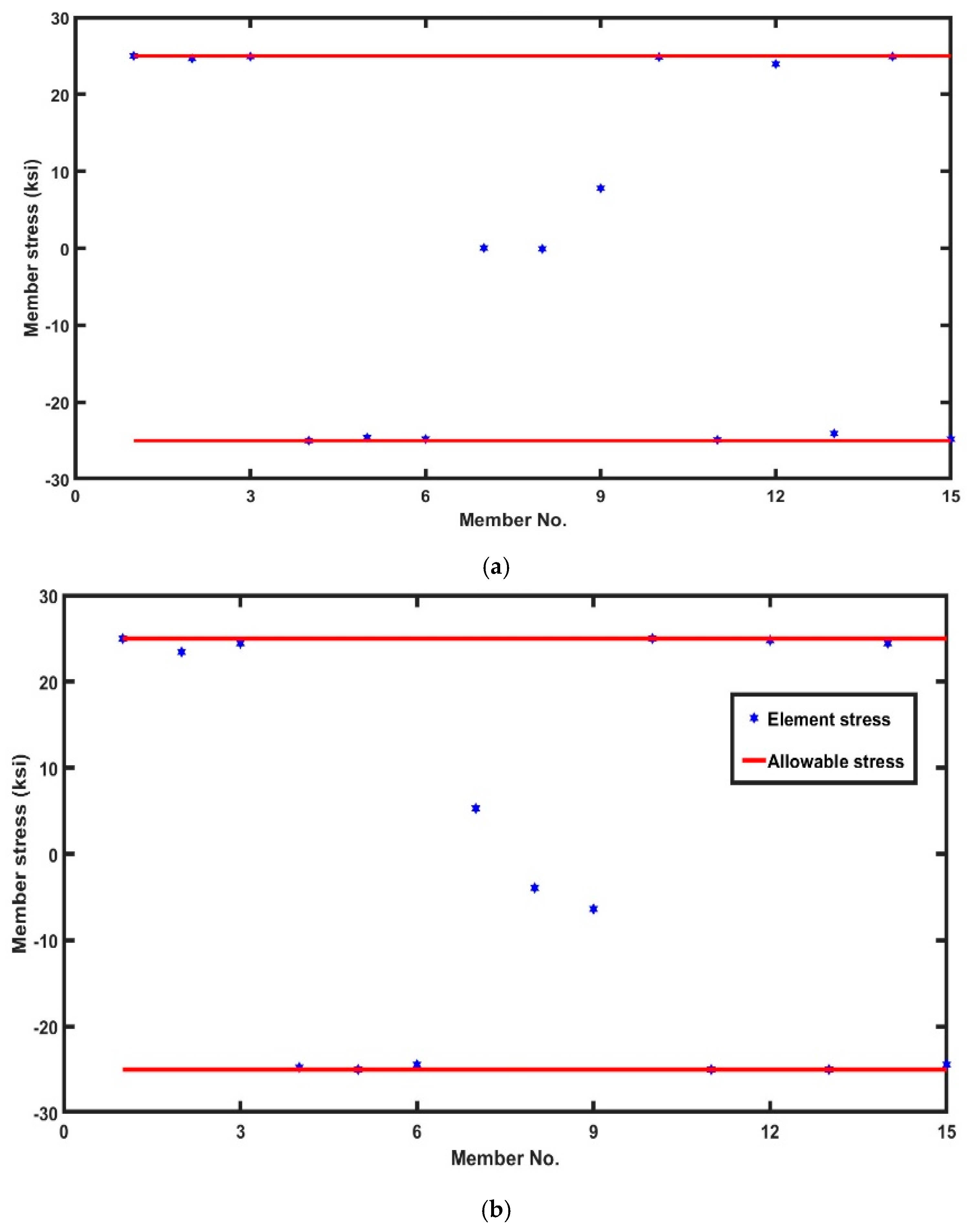
5.1. The 15-Bar Planar Truss
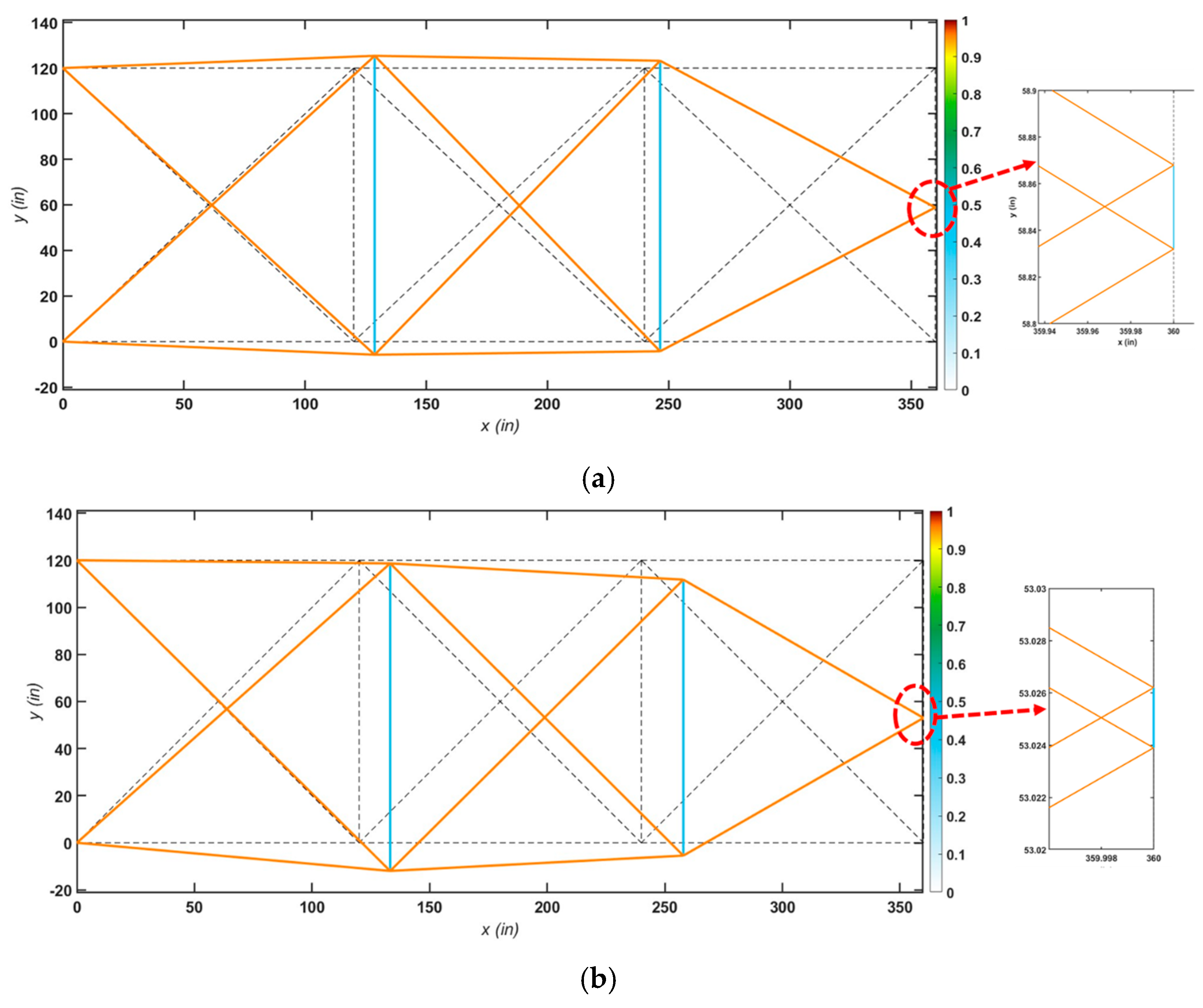
5.2. The 18-Bar Planar Truss
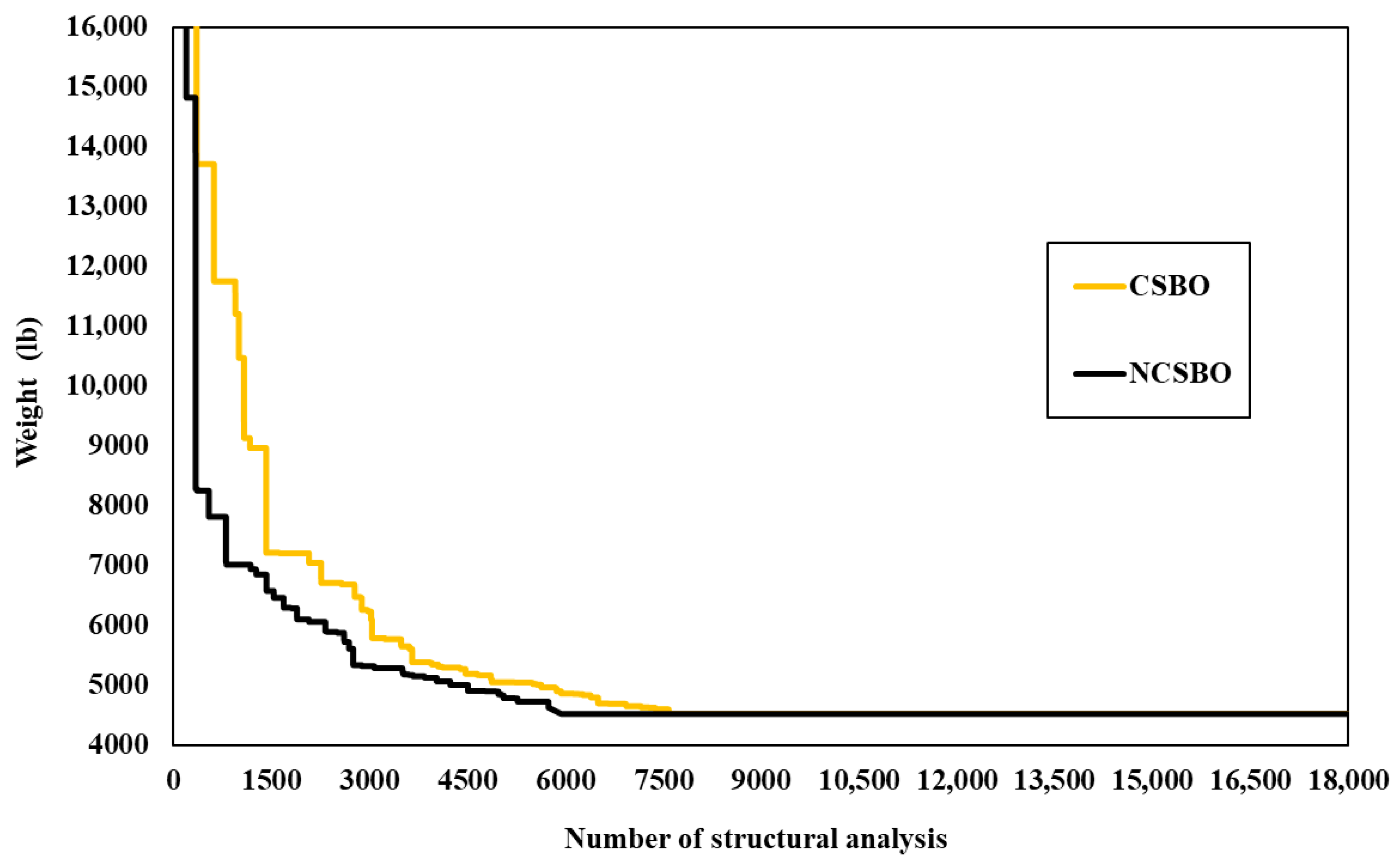
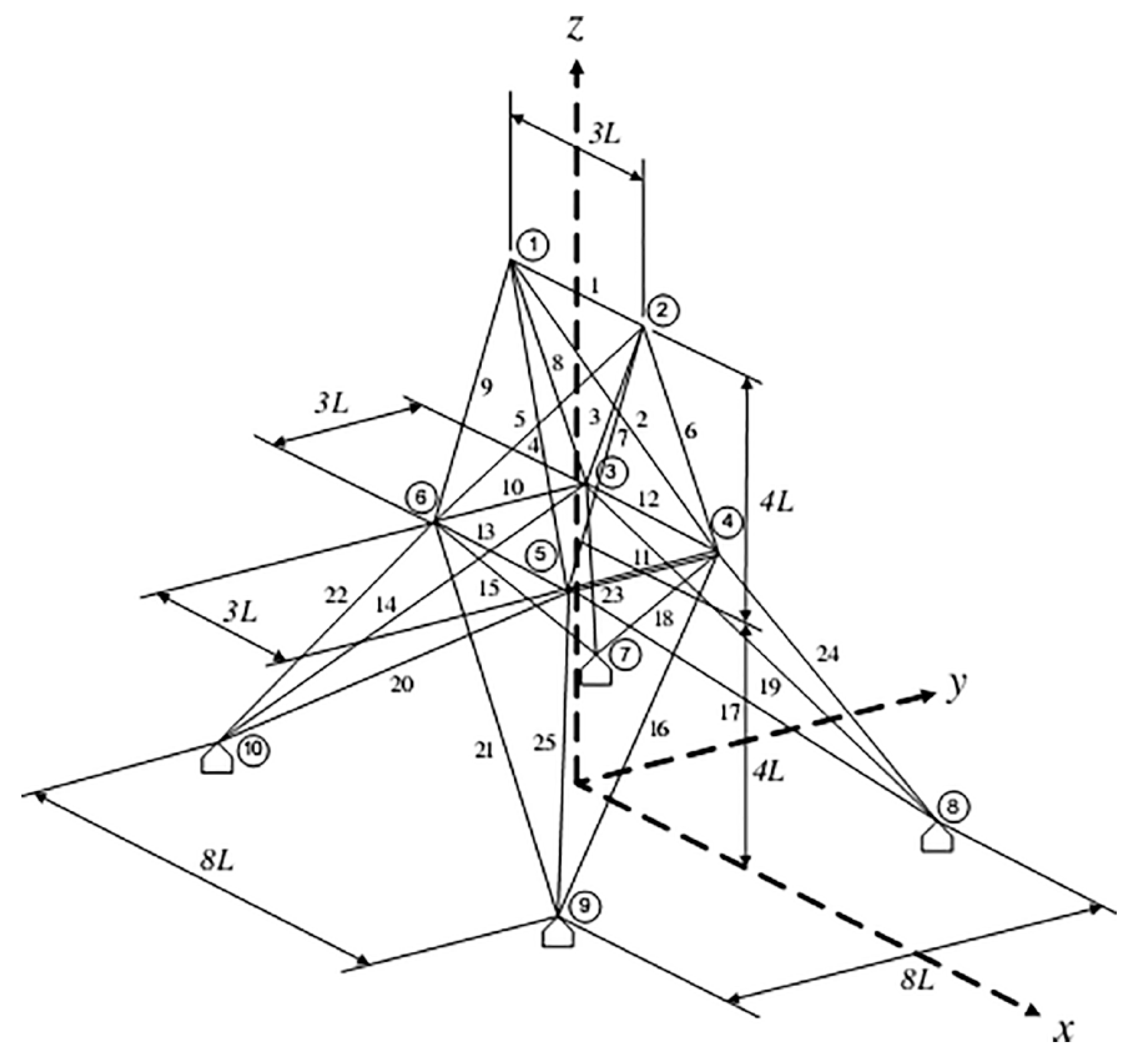
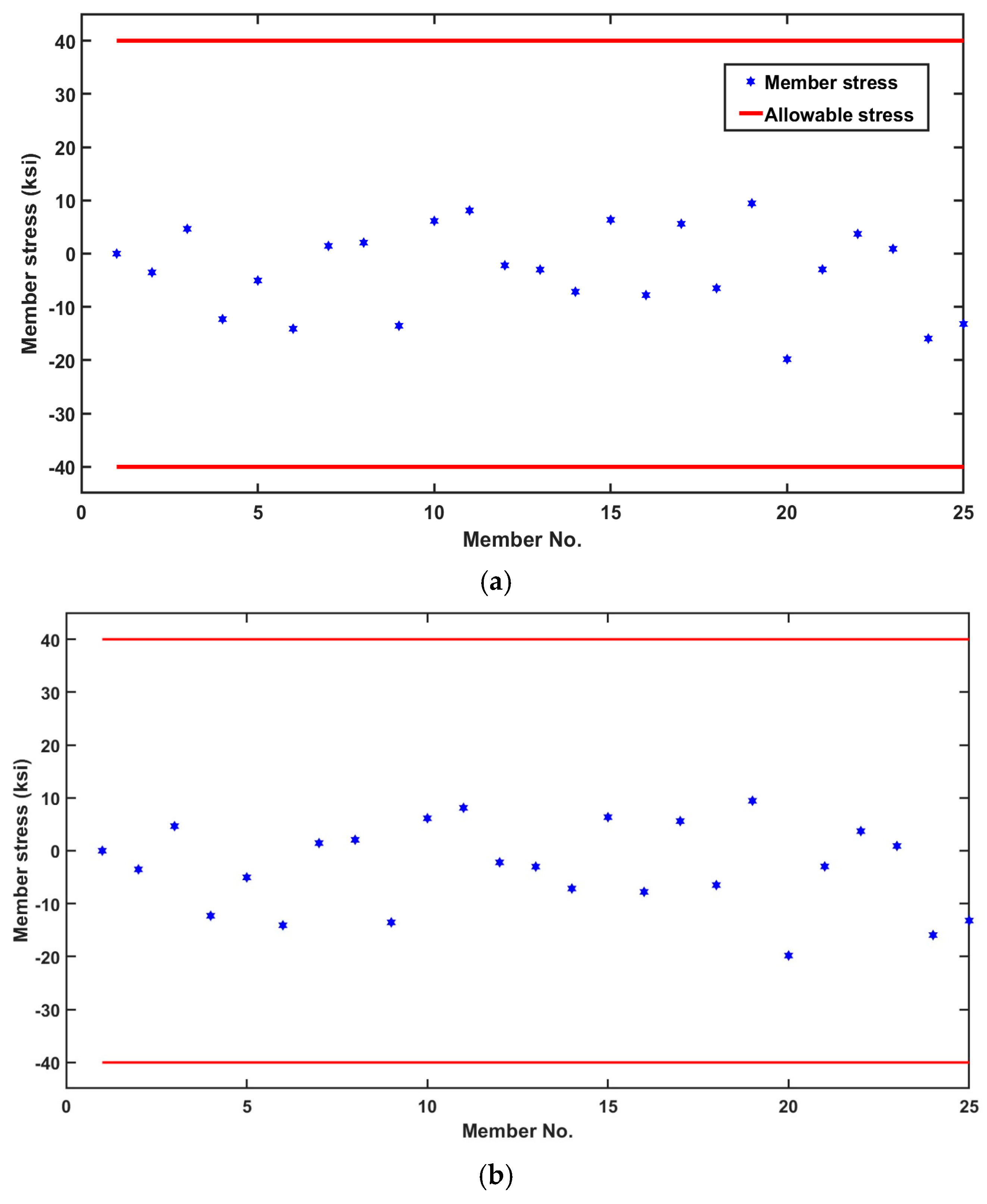
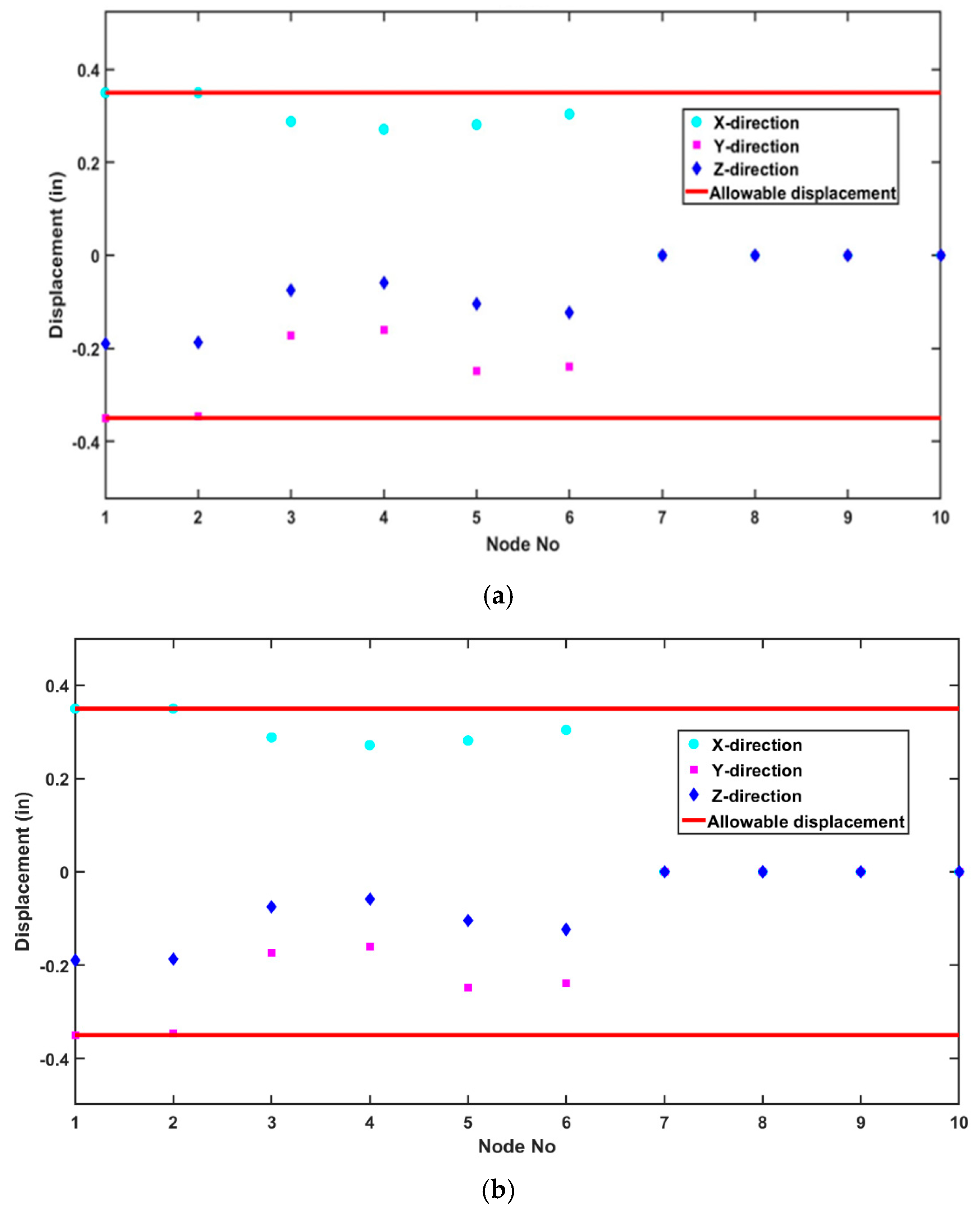
5.3. The 25-Bar Planar Truss
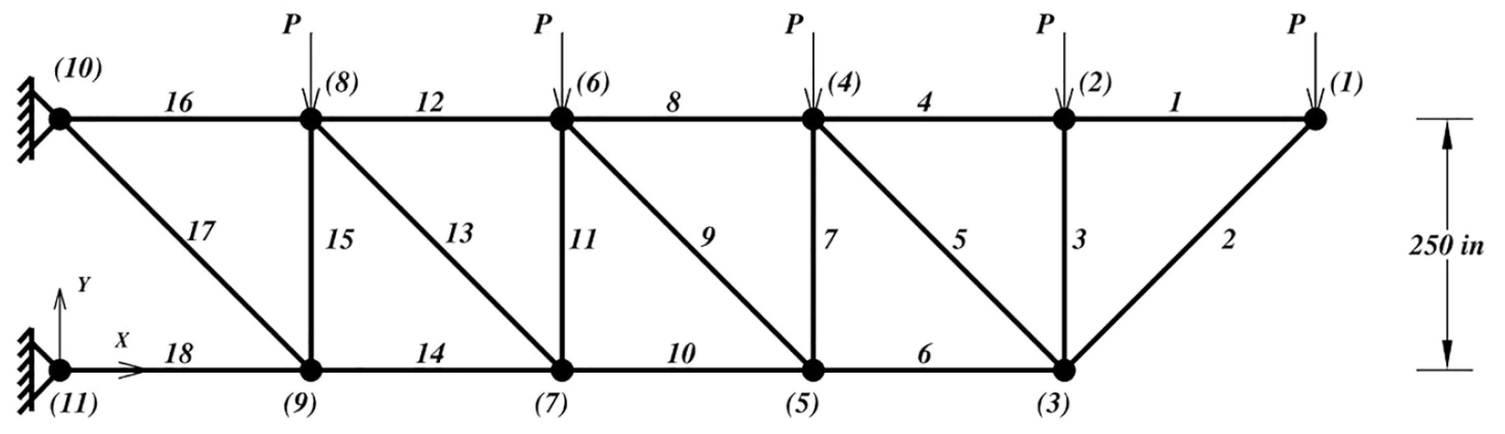
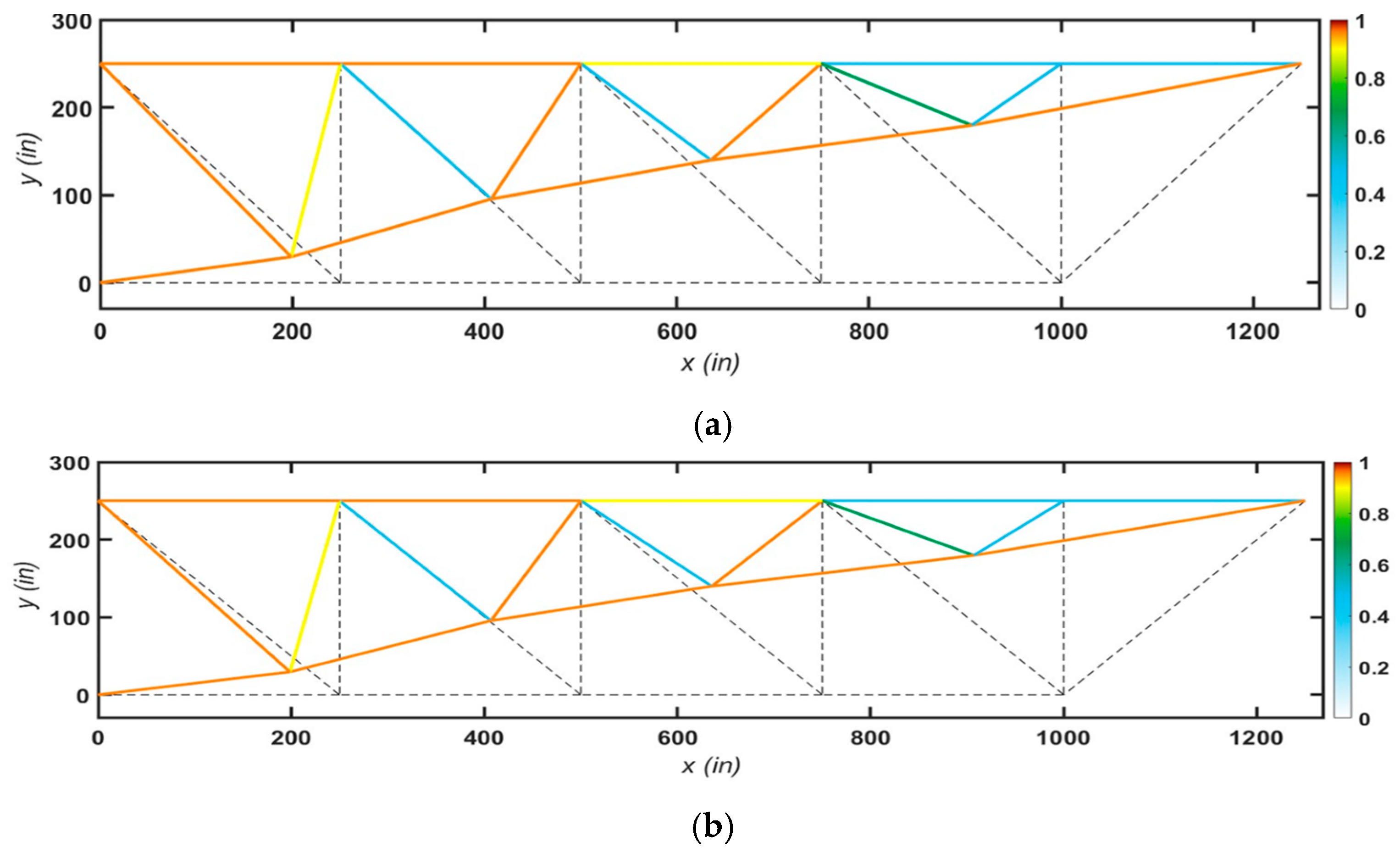
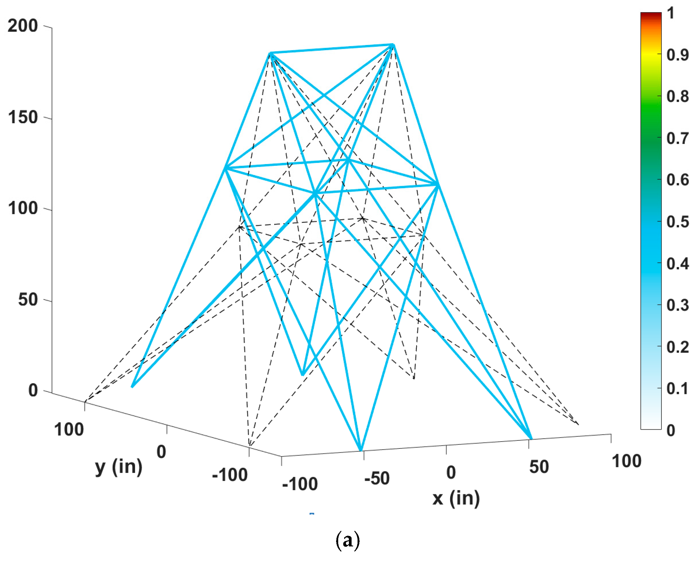
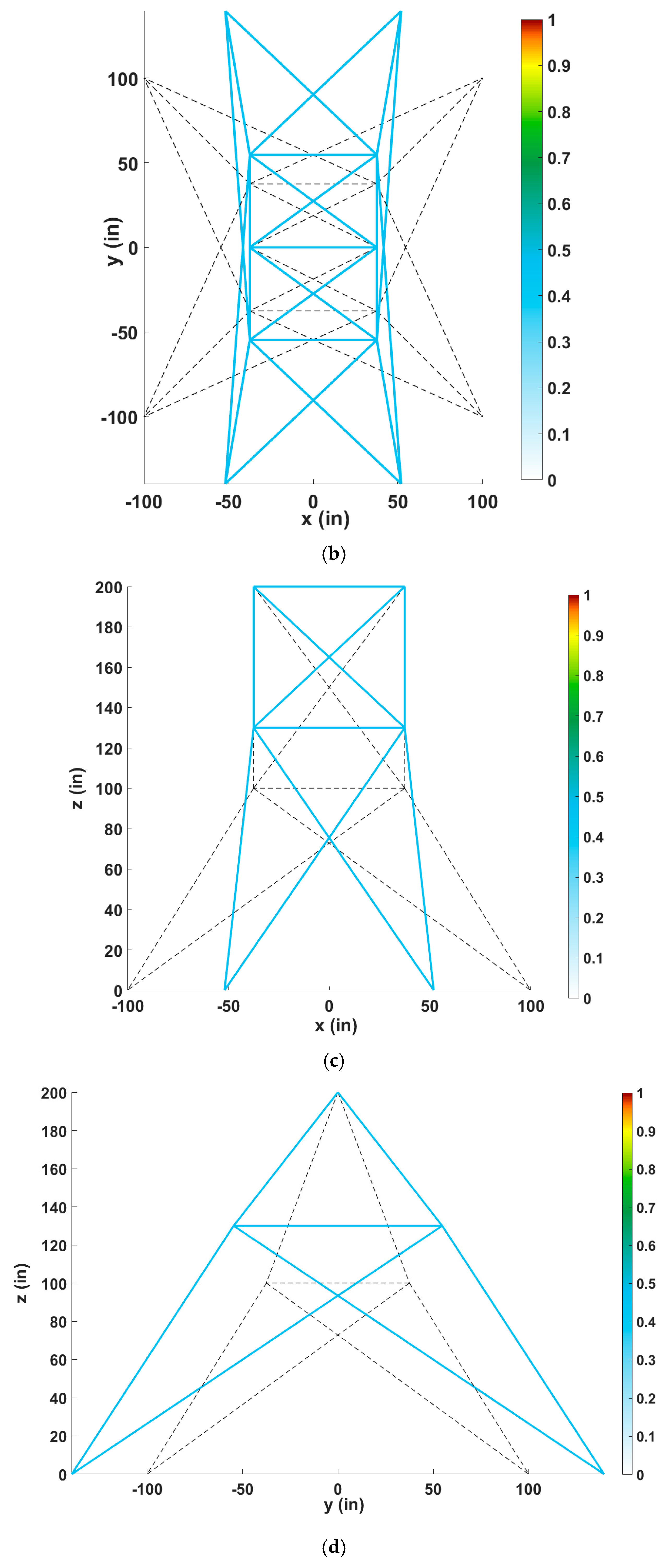
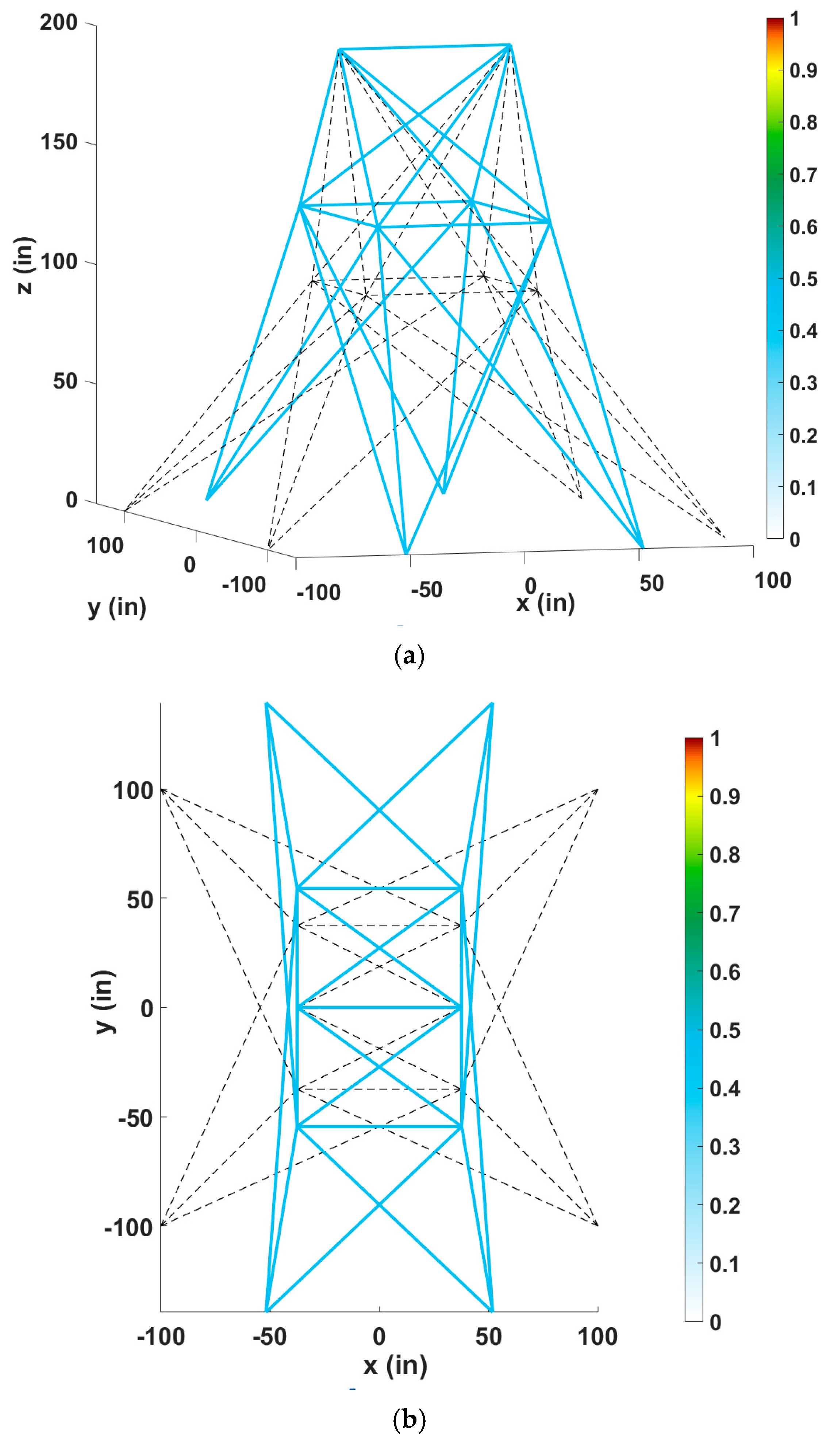
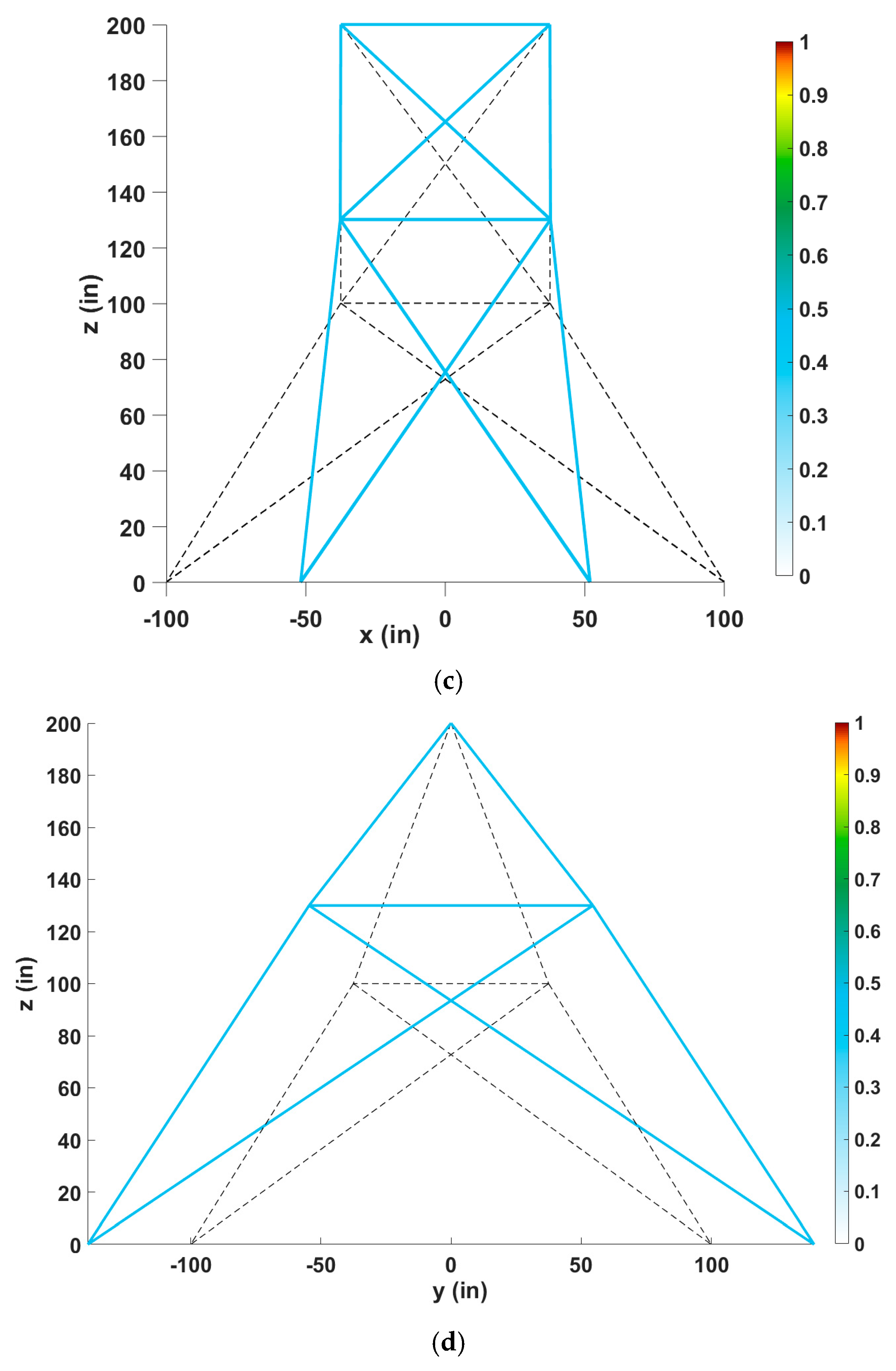
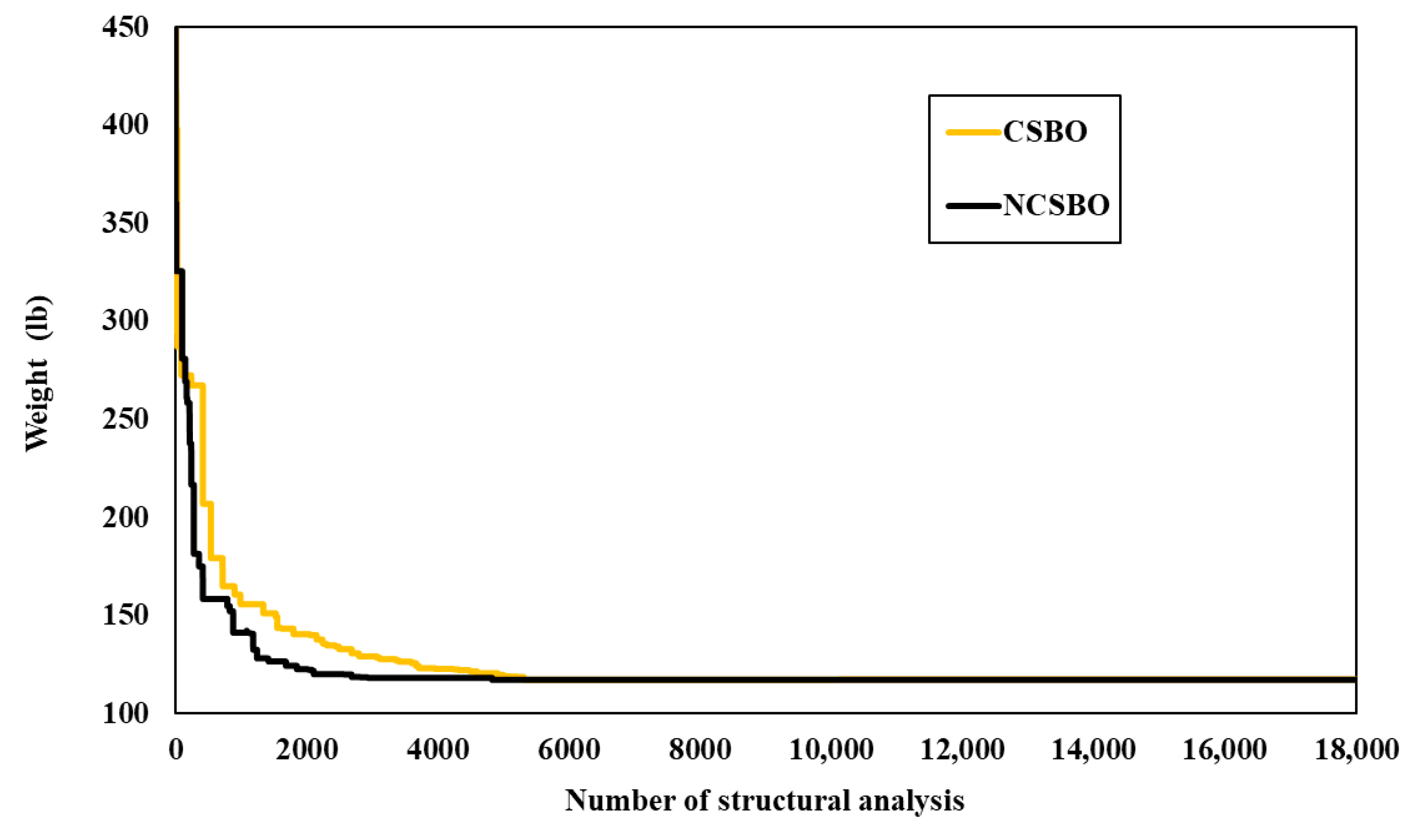
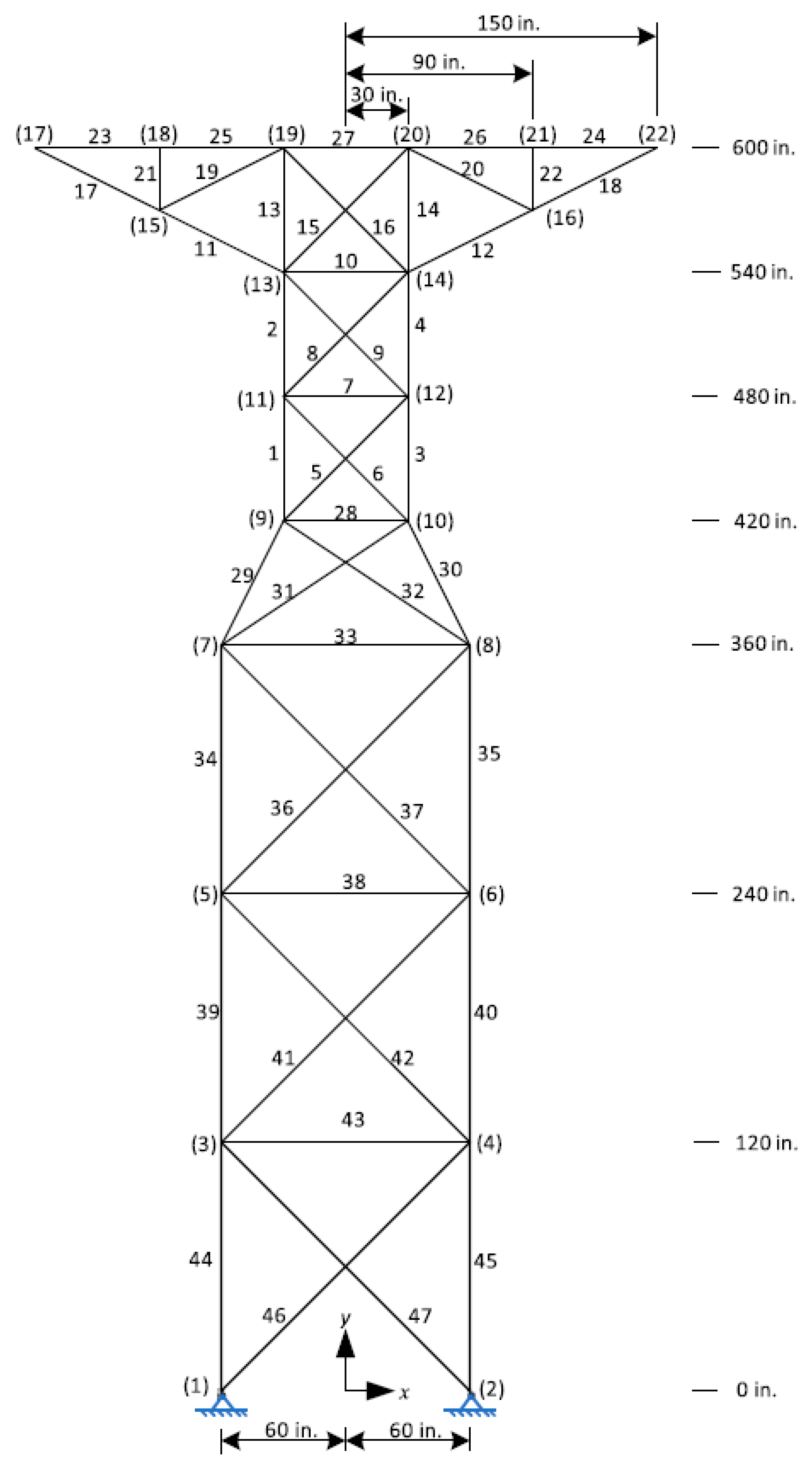
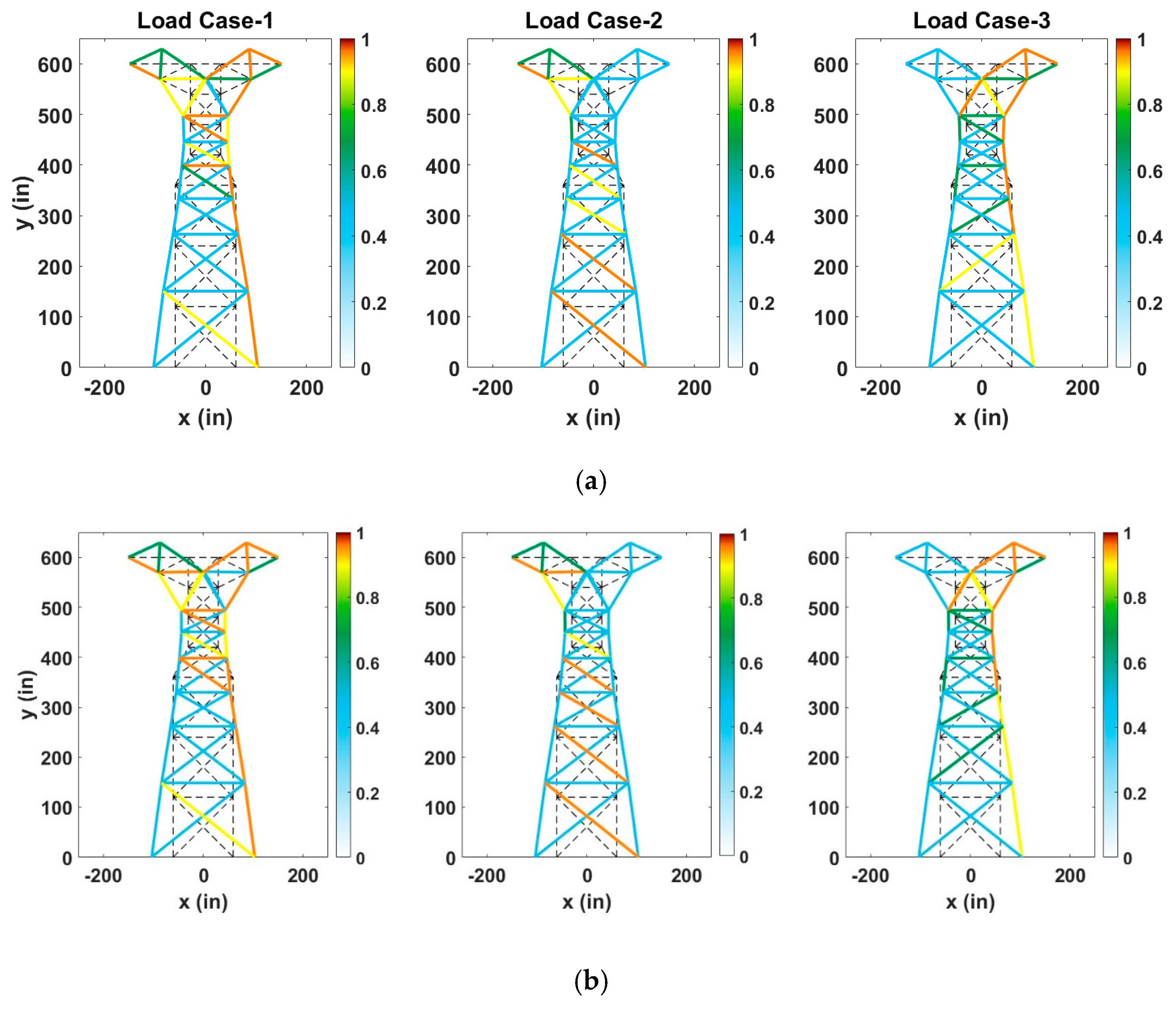
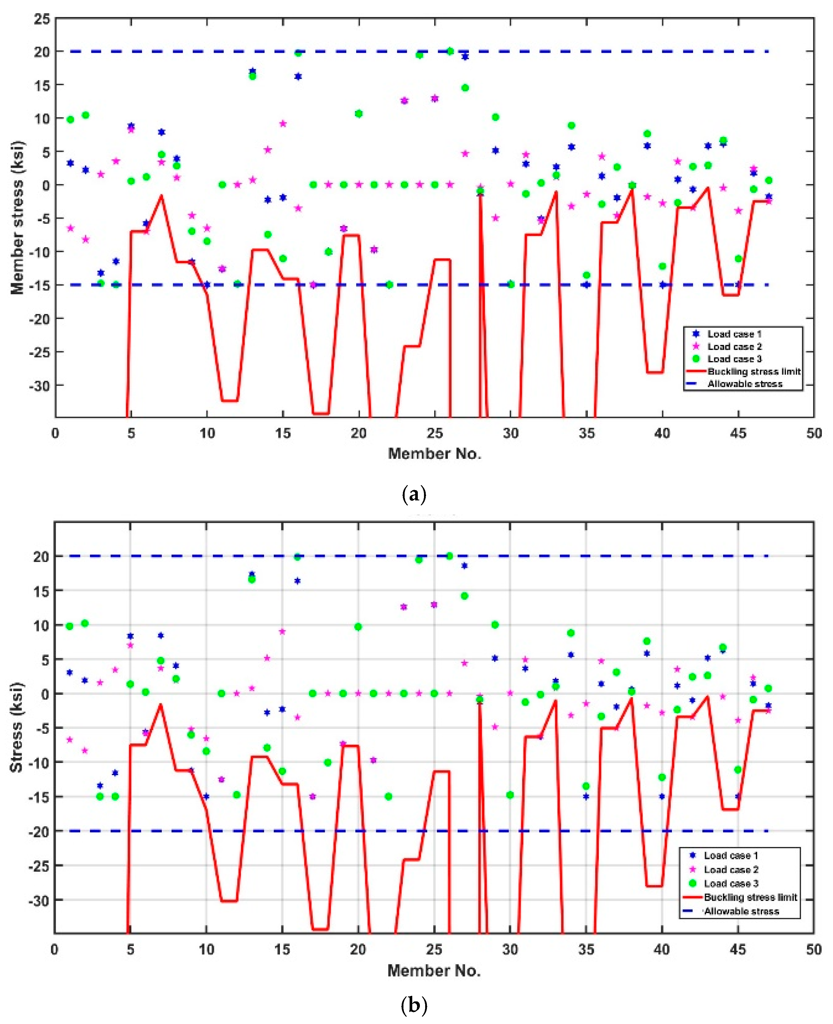
5.4. The 47-Bar Planar Truss
| Sizing variables | A3 = A1; A4 = A2; A5 = A6; A7; A8 = A9; A10; A12 = A11; A14 = A13; A15 = A16; A18 = A17; A20 = A19; A22 = A21; A24 = A23; A26 = A25; A27; A28; A30 = A29; A31 = A32; A33; A35 = A34; A36 = A37; A38; A40 = A39; A41 = A42; A43; A45 = A44; A46 = A47 |
| Layout variables | x2 = −x1; x4 = −x3; y4 = y3; x6 = −x5; y6 = y5; x8 = −x7; y8 = y7; x10 = −x9; y10 = y9; x12 = −x11; y12 = y11; x14 = −x13; y14 = y13; x20 = −x19; y20 = y19; x21 = −x18; y21 = y18 |
6. Conclusions
Author Contributions
Funding
Institutional Review Board Statement
Informed Consent Statement
Data Availability Statement
Conflicts of Interest
References
- Holland, J.H. Adaptation in Natural and Artificial Systems; University of Michigan Press: Ann Arbor, MI, USA, 1975. [Google Scholar]
- Kirkpatrick, S.; Gelatt, C.D., Jr.; Vecchi, M.P. Optimization By Simulated Annealing. Science 1983, 220, 671–680. [Google Scholar] [CrossRef] [PubMed]
- Glover, F. Future Paths for Integer Programming and Links to Artificial Intelligence. Comput. Oper. Res. 1986, 13, 533–549. [Google Scholar] [CrossRef]
- Kennedy, J.; Eberhart, R. Particle swarm optimization. In Proceedings of the IEEE International Conference on Neural Networks, Perth, WA, Australia, 27 November–1 December 1995; Volume 4. [Google Scholar] [CrossRef]
- Dorigo, M.; Maniezzo, V.; Colorni, A. Ant system: Optimization by a colony of cooperating agents. IEEE Trans. Syst. MAN Cybern. PART B-CYBERNETICS 1996, 26, 29–41. [Google Scholar] [CrossRef]
- Geem, Z.W.; Kim, J.H.; Loganathan, G.V. A new heuristic optimization algorithm: Harmony search. Simulation 2001, 76, 60–68. [Google Scholar] [CrossRef]
- Erol, O.K.; Eksin, I. A new optimization method: Big Bang Big Crunch. Adv. Eng. Softw. 2006, 37, 106–111. [Google Scholar] [CrossRef]
- Karaboga, D.; Basturk, B. A powerful and efficient algorithm for numerical function optimization: Artificial bee colony (ABC) algorithm. J. Glob. Optim. 2007, 39, 459–471. [Google Scholar] [CrossRef]
- Yang, X.-S.; Deb, S. Engineering optimization by cuckoo search. Int. J. Math. Model. Numer. Optim. 2010, 1, 330–343. [Google Scholar] [CrossRef]
- Rao, R.V.; Savsani, V.J.; Vakharia, D.P. Teaching-learning-based optimization: A novel method for constrained mechanical design optimization problems. Comput. Des. 2011, 43, 303–315. [Google Scholar] [CrossRef]
- Mirjalili, S.; Mirjalili, S.M.; Lewis, A. Grey Wolf Optimizer. Adv. Eng. Softw. 2014, 69, 46–61. [Google Scholar] [CrossRef]
- Mirjalili, S. Moth-flame optimization algorithm: A novel nature-inspired heuristic paradigm. Knowl. Based Syst. 2015, 89, 228–249. [Google Scholar] [CrossRef]
- Askarzadeh, A. A novel metaheuristic method for solving constrained engineering optimization problems: Crow search algorithm. Comput. Struct. 2016, 169, 1–12. [Google Scholar] [CrossRef]
- Rao, R.V. Jaya: A simple and new optimization algorithm for solving constrained and unconstrained optimization problems. Int. J. Ind. Eng. Comput. 2016, 7, 19–34. [Google Scholar] [CrossRef]
- Arora, S.; Singh, S. Butterfly optimization algorithm: A novel approach for global optimization. Soft Comput. 2019, 23, 715–734. [Google Scholar] [CrossRef]
- Hashim, F.A.; Houssein, E.H.; Mabrouk, M.S.; Al-Atabany, W.; Mirjalili, S. Henry gas solubility optimization: A novel physics-based algorithm. Futur. Gener. Comp. Syst. 2019, 101, 646–667. [Google Scholar] [CrossRef]
- Faramarzi, A.; Heidarinejad, M.; Stephens, B.; Mirjalili, S. Equilibrium optimizer: A novel optimization algorithm. Knowl. Based Syst. 2020, 191, 105190. [Google Scholar] [CrossRef]
- Li, S.M.; Chen, H.L.; Wang, M.J.; Heidari, A.A.; Mirjalili, S. Slime mould algorithm: A new method for stochastic optimization. Futur. Gener. Comp. Syst. 2020, 111, 300–323. [Google Scholar] [CrossRef]
- Abualigah, L.; Yousri, D.; Elaziz, M.A.; Ewees, A.A.; Al-Qaness, M.A.; Gandomi, A.H. Aquila Optimizer: A novel meta-heuristic optimization algorithm. Comput. Ind. Eng. 2021, 157, 107250. [Google Scholar] [CrossRef]
- Braik, M.; Hammouri, A.; Atwan, J.; Al-Betar, M.A.; Awadallah, M.A. White Shark Optimizer: A novel bio-inspired meta-heuristic algorithm for global optimization problems. Knowl. Based Syst. 2022, 243, 108457. [Google Scholar] [CrossRef]
- Ghasemi, M.; Akbari, M.-A.; Jun, C.; Bateni, S.M.; Zare, M.; Zahedi, A.; Pai, H.-T.; Band, S.S.; Moslehpour, M.; Chau, K.-W. Circulatory System Based Optimization (CSBO): An expert multilevel biologically inspired meta-heuristic algorithm. Eng. Appl. Comput. Fluid. Mech. 2022, 16, 1483–1525. [Google Scholar] [CrossRef]
- Agushaka, J.O.; Ezugwu, A.E.; Abualigah, L. Gazelle optimization algorithm: A novel nature-inspired metaheuristic optimizer. Neural Comput. Appl. 2023, 35, 4099–4131. [Google Scholar] [CrossRef]
- Abdel-Basset, M.; Abdel-Fatah, L.; Sangaiah, A.K. Metaheuristic Algorithms: A Comprehensive Review. In Computational Intelligence for Multimedia Big Data on the Cloud with Engineering Applications; Sangaiah, A.K., Sheng, M., Zhang, Z., Eds.; A volume in Intelligent Data-Centric Systems; Intelligent Data-Centric Systems; Academic Press: Cambridge, MA, USA, 2018; pp. 185–231. [Google Scholar] [CrossRef]
- Rajwar, K.; Deep, K.; Das, S. An exhaustive review of the metaheuristic algorithms for search and optimization: Taxonomy, applications, and open challenges. Artif. Intell. Rev. 2023, 56, 13187–13257. [Google Scholar] [CrossRef] [PubMed]
- Alorf, A. A survey of recently developed metaheuristics and their comparative analysis. Eng. Appl. Arti Intel. 2023, 117, 105622. [Google Scholar] [CrossRef]
- Li, G.; Zhang, T.; Tsai, C.-Y.; Yao, L.; Lu, Y.; Tang, J. Review of the metaheuristic algorithms in applications: Visual analysis based on bibliometrics. Expert. Syst. Appl. 2024, 255, 124857. [Google Scholar] [CrossRef]
- Martí, R.; Sevaux, M.; Sörensen, K. Fifty years of metaheuristics. Eur. J. Oper. Res. 2025, 321, 345–362. [Google Scholar] [CrossRef]
- Wu, S.J.; Chow, P.T. Integrated discrete and configuration optimization of trusses using genetic algorithms. Comput. Struct. 1995, 55, 695–702. [Google Scholar] [CrossRef]
- Soh, C.K.; Yang, J. Fuzzy controlled genetic algorithm search for shape optimization. J. Comput. Civ. Eng. 1996, 10, 143–150. [Google Scholar] [CrossRef]
- Kaveh, A.; Talatahari, S. An enhanced charged system search for configuration optimization using concept of fields of forces. Struct. Multidiscip. Optim. 2011, 43, 339–351. [Google Scholar] [CrossRef]
- Fadel Miguel, L.F.; Fadel Miguel, L.F. Shape and size optimization of truss structures considering dynamic constraints through modern metaheuristic algorithms. Expert. Syst. Appl. 2012, 39, 9458–9467. [Google Scholar] [CrossRef]
- Kazemzadeh Azad, S.; Bybordiani, M.; Kazemzadeh Azad Sinaand Jawad, F.K.J. Simultaneous size and geometry optimization of steel trusses under dynamic excitations. Struct. Multidiscip. Optim. 2018, 58, 2545–2563. [Google Scholar] [CrossRef]
- Grzywiński, M.; Selejdak, J.; Dede, T. Shape and size optimization of trusses with dynamic constraints using a metaheuristic algorithm. Steel Compos. Struct. 2019, 33, 747–753. [Google Scholar] [CrossRef]
- Varma, T.V.; Sarkar, S.; Mondal, G. Buckling Restrained Sizing and Shape Optimization of Truss Structures. J. Struct. Eng. 2020, 146, 04020048. [Google Scholar] [CrossRef]
- Eid, H.F.; Garcia-Hernandez, L.; Abraham, A. Spiral water cycle algorithm for solving multi-objective optimization and truss optimization problems. Eng. Comput. 2022, 38, 963–973. [Google Scholar] [CrossRef]
- Azizi, M.; Shishehgarkhaneh, M.B.; Basiri, M. Optimum design of truss structures by Material Generation Algorithm with discrete variables. Decis. Anal. J. 2022, 3, 100043. [Google Scholar] [CrossRef]
- Delyová, I.; Frankovský, P.; Bocko, J.; Trebuňa, P.; Živčák, J.; Schürger, B.; Janigová, S. Sizing and topology optimization of trusses using genetic algorithm. Materials 2021, 14, 715. [Google Scholar] [CrossRef] [PubMed]
- Pierezan, J.; Coelho, L.d.S.; Mariani, V.C.; Segundo, E.H.d.V.; Prayogo, D. Chaotic coyote algorithm applied to truss optimization problems. Comput. Struct. 2021, 242, 106353. [Google Scholar] [CrossRef]
- Kaveh, A.; Zaerreza, A. Size/layout optimization of truss structures using shuffled shepherd optimization method. Period Polytech. Civ. Eng. 2020, 64, 408–421. [Google Scholar] [CrossRef]
- Pham, H.A.; Tran, T.D. Optimal truss sizing by modified Rao algorithm combined with feasible boundary search method. Expert. Syst. Appl. 2022, 191, 116337. [Google Scholar] [CrossRef]
- Rao, R.V. Rao algorithms: Three metaphor-less simple algorithms for solving optimization problems. Int. J. Ind. Eng. Comput. 2020, 11, 107–130. [Google Scholar] [CrossRef]
- Degertekin, S.O.; Minooei, M.; Santoro, L.; Trentadue, B.; Lamberti, L. Large-scale truss-sizing optimization with enhanced hybrid hs algorithm. Appl. Sci. 2021, 11, 3270. [Google Scholar] [CrossRef]
- Kooshkbaghi, M.; Kaveh, A. Sizing Optimization of Truss Structures with Continuous Variables by Artificial Coronary Circulation System Algorithm. Iran. J. Sci. Technol. Trans. Civ. Eng. 2020, 44, 1–20. [Google Scholar] [CrossRef]
- Panagant, N.; Pholdee, N.; Bureerat, S.; Yildiz, A.R.; Mirjalili, S. A Comparative Study of Recent Multi-objective Metaheuristics for Solving Constrained Truss Optimisation Problems. Arch. Comput. Methods Eng. 2021, 28, 4031–4047. [Google Scholar] [CrossRef]
- Kaveh, A.; Khosravian, M. Size/Layout Optimization of Truss Structures Using Vibrating Particles System Meta-heuristic Algorithm and its Improved Version. Period. Polytech. Civ. Eng. 2022, 66, 1–17. [Google Scholar] [CrossRef]
- Awad, R. Sizing optimization of truss structures using the political optimizer (PO) algorithm. Structures 2021, 33, 4871–4894. [Google Scholar] [CrossRef]
- Askari, Q.; Younas, I.; Saeed, M. Political Optimizer: A novel socio-inspired meta-heuristic for global optimization. Knowl. Based Syst. 2020, 195, 105709. [Google Scholar] [CrossRef]
- Lamberti, L.; Pappalettere, C. Metaheuristic Design Optimization of Skeletal Structures: A Review. Comput. Technol. Rev. 2010, 4, 1–32. [Google Scholar] [CrossRef]
- Stolpe, M. Truss optimization with discrete design variables: A critical review. Struct. Multidisc Optim. 2016, 53, 349–374. [Google Scholar] [CrossRef]
- Renkavieski, C.; Parpinelli, R.S. Meta-heuristic algorithms to truss optimization: Literature mapping and application. Expert. Syst. Appl. 2021, 182, 115197. [Google Scholar] [CrossRef]
- Kashani, A.R.; Camp, C.V.; Rostamian, M.; Azizi, K.; Gandomi, A.H. Population-based optimization in structural engineering: A review. Artif. Intell. Rev. 2022, 55, 345–452. [Google Scholar] [CrossRef]
- Etaati, B.; Dehkordi, A.A.; Sadollah, A.; El-Abd, M.; Neshat, M. Comparative State-of-the-Art Constrained Metaheuristics Framework for TRUSS Optimisation on Shape and Sizing. Math. Probl. Eng. 2022, 2022, 6078986. [Google Scholar] [CrossRef]
- AISC-LRFD. Manual of steel construction-Load and Resistance Factor Design. In LRFD, 2nd ed.; American Institute of Steel Construction: Chicago, IL, USA, 2001. [Google Scholar]
- Rahami, H.; Kaveh, A.; Gholipour, Y. Sizing, geometry and topology optimization of trusses via force method and genetic algorithm. Eng. Struct. 2008, 30, 2360–2369. [Google Scholar] [CrossRef]
- Hwang, S.-F.; He, R.-S. A hybrid real-parameter genetic algorithm for function optimization. Adv. Eng. Inform. 2006, 20, 7–21. [Google Scholar] [CrossRef]
- Gholizadeh, S. Layout optimization of truss structures by hybridizing cellular automata and particle swarm optimization. Comput. Struct. 2013, 125, 86–99. [Google Scholar] [CrossRef]
- Tang, W.Y.; Tong, L.Y.; Gu, Y.X. Improved genetic algorithm for design optimization of truss structures with sizing, shape and topology variables. Int. J. Numer. Methods Eng. 2005, 62, 1737–1762. [Google Scholar] [CrossRef]
- Fadel Miguel, L.F.; Lopez, R.H.; Fadel Miguel, L.F. Multimodal size, shape, and topology optimization of truss structures using the Firefly algorithm. Adv. Eng. Softw. 2013, 56, 23–37. [Google Scholar] [CrossRef]
- Dede, T.; Ayvaz, Y. Combined size and shape optimization of structures with a new meta-heuristic algorithm. Appl. Soft Comput. 2015, 28, 250–258. [Google Scholar] [CrossRef]
- Gholizadeh, S.; Barzegar, A.; Gheyratmand, C. Shape Optimization of Structures By Modified Harmony Search. Int. J. Optim. Civ. Eng. 2011, 1, 485–494. [Google Scholar]
- Ho-Huu, V.; Nguyen-Thoi, T.; Nguyen-Thoi, M.; Le-Anh, L. An improved constrained differential evolution using discrete variables(D-ICDE) for layout optimization of truss structures. Expert. Syst. Appl. 2015, 42, 7057–7069. [Google Scholar] [CrossRef]
- Jawad, F.K.; Ozturk, C.; Dansheng, W.; Mahmood, M.; Al-Azzawi, O.; Al-Jemely, A. Sizing and layout optimization of truss structures with artificial bee colony algorithm. Structures 2021, 30, 546–559. [Google Scholar] [CrossRef]
- He, S.X.; Cui, Y.T. Medalist learning algorithm for configuration optimization of trusses. Appl. Soft Comput. 2023, 148, 110889. [Google Scholar] [CrossRef]
- Rajeev, S.; Krishnamoorthy, C.S. Genetic algorithms-based methodologies for design optimization of trusses. J. Struct. Eng. 1997, 123, 350–358. [Google Scholar] [CrossRef]
- Kaveh, A.; Kalatjari, V. Size/geometry optimization of trusses by the force method and genetical algorithm. Z. Fur Angew. Math. Und Mech. 2004, 84, 347–357. [Google Scholar] [CrossRef]
- Li, L.; Liu, F. Group Search Optimization for Applications in Structural Design. Gr. SEARCH Optim. Appl. Struct. Des. 2011, 9, 1–249. [Google Scholar] [CrossRef]
- Salajegheh, E.; Vanderplaats, G.N. Optımum Desıgn of Trusses with Dıscrete Sızıng and Shape Varıables. Struct. Optim. 1993, 6, 79–85. [Google Scholar] [CrossRef]
- Hasançebi, O.; Erbatur, F. Layout optimization of trusses using improved GA methodologies. Acta Mech. 2001, 146, 87–107. [Google Scholar] [CrossRef]


| Parameter or Function in NCSBO | The Equivalent Concept in This Paper |
|---|---|
| Blood mass | Steel truss |
| The movement of blood in the body | Modifying the sizing and shape variables of truss designs |
| Circulation cycle | Iteration |
| Deoxygenated blood | Heavier truss designs |
| Oxygenated blood | Lighter truss designs |
| Purification of blood | Composition of high- and low-cost truss designs |
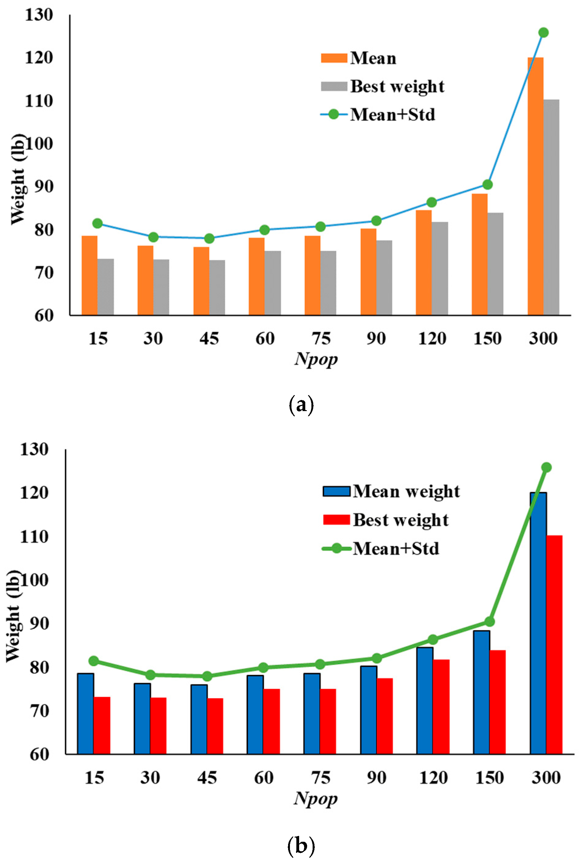
| NCSBO | |||||||||
|---|---|---|---|---|---|---|---|---|---|
| Npop | 15 | 30 | 45 | 60 | 75 | 90 | 120 | 150 | 300 |
| Best weight (lb *) | 74.388 | 72.946 | 72.688 | 73.742 | 75.491 | 76.713 | 81.030 | 83.963 | 106.672 |
| Mean (lb) | 78.745 | 76.891 | 75.92 | 76.555 | 78.890 | 80.002 | 84.043 | 88.110 | 118.454 |
| Std (lb) | 2.197 | 2.061 | 1.966 | 2.131 | 1.516 | 1.854 | 1.686 | 1.899 | 5.744 |
| Mean + Std (lb) | 80.942 | 78.952 | 77.886 | 78.686 | 80.407 | 81.856 | 85.730 | 90.008 | 124.199 |
| CSBO | |||||||||
| Npop | 15 | 30 | 45 | 60 | 75 | 90 | 120 | 150 | 300 |
| Best weight (lb) | 73.177 | 73.048 | 72.843 | 75.051 | 75.038 | 77.52 | 81.789 | 83.953 | 110.311 |
| Mean (lb) | 78.61 | 76.275 | 76.452 | 78.102 | 78.577 | 80.207 | 84.488 | 88.349 | 120.024 |
| Std (lb) | 2.845 | 2 | 2.116 | 1.917 | 2.188 | 1.882 | 1.894 | 2.187 | 5.863 |
| Mean + Std (lb) | 81.455 | 78.275 | 78.568 | 80.019 | 80.765 | 82.089 | 86.382 | 90.536 | 125.887 |
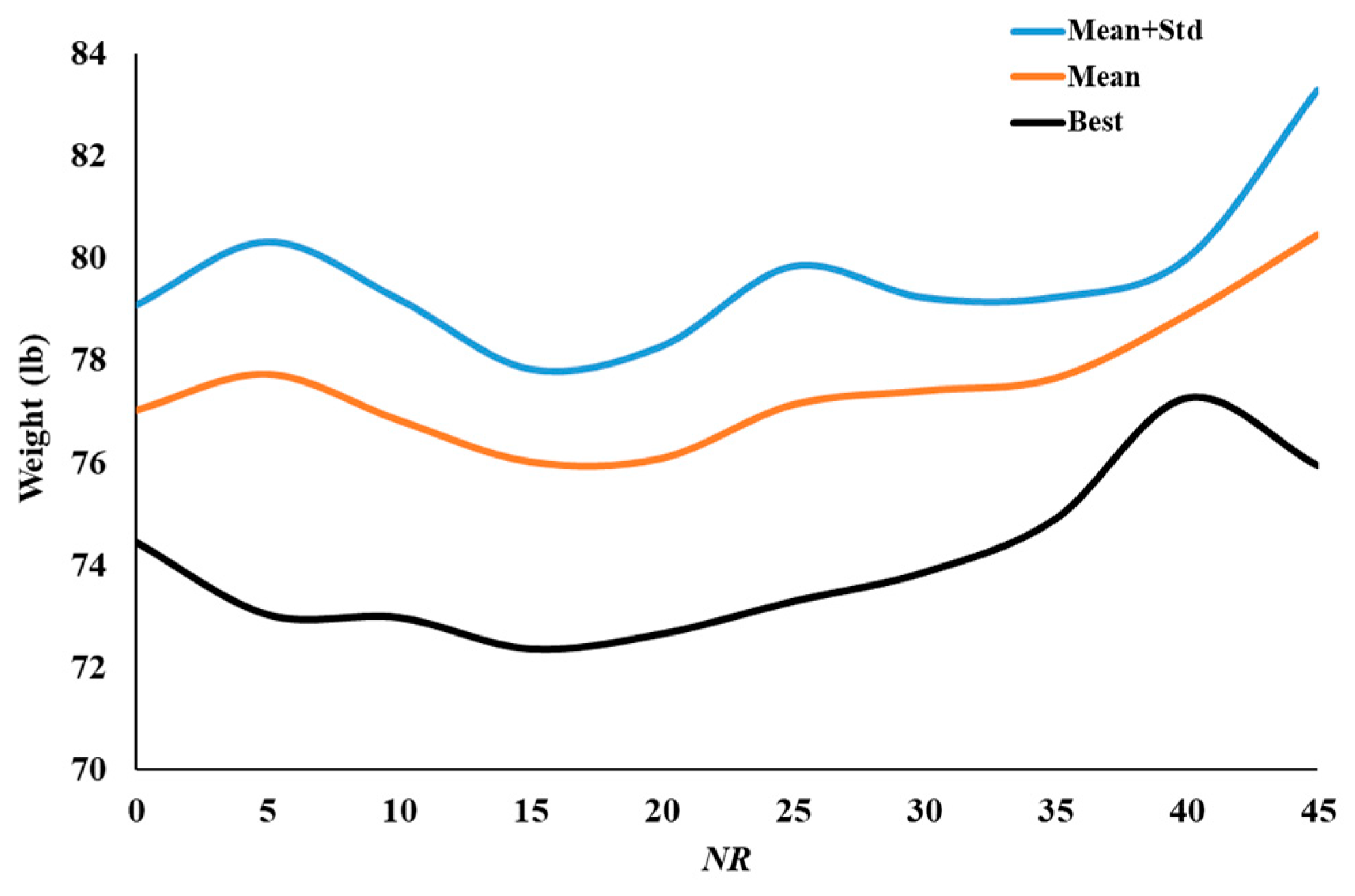
| NR | 0 | 5 | 10 | 15 | 20 | 25 | 30 | 35 | 40 | 45 |
|---|---|---|---|---|---|---|---|---|---|---|
| Best weight (lb) | 74.434 | 73.019 | 72.963 | 72.348 | 72.641 | 73.275 | 73.842 | 74.881 | 77.250 | 75.932 |
| Mean (lb) | 77.031 | 77.735 | 76.835 | 76.024 | 76.088 | 77.136 | 77.410 | 77.654 | 78.890 | 80.458 |
| Std (lb) | 2.049 | 2.578 | 2.359 | 1.805 | 2.183 | 2.700 | 1.812 | 1.575 | 1.091 | 2.822 |
| Mean + Std (lb) | 79.080 | 80.313 | 79.194 | 77.829 | 78.271 | 79.836 | 79.222 | 79.229 | 79.982 | 83.280 |
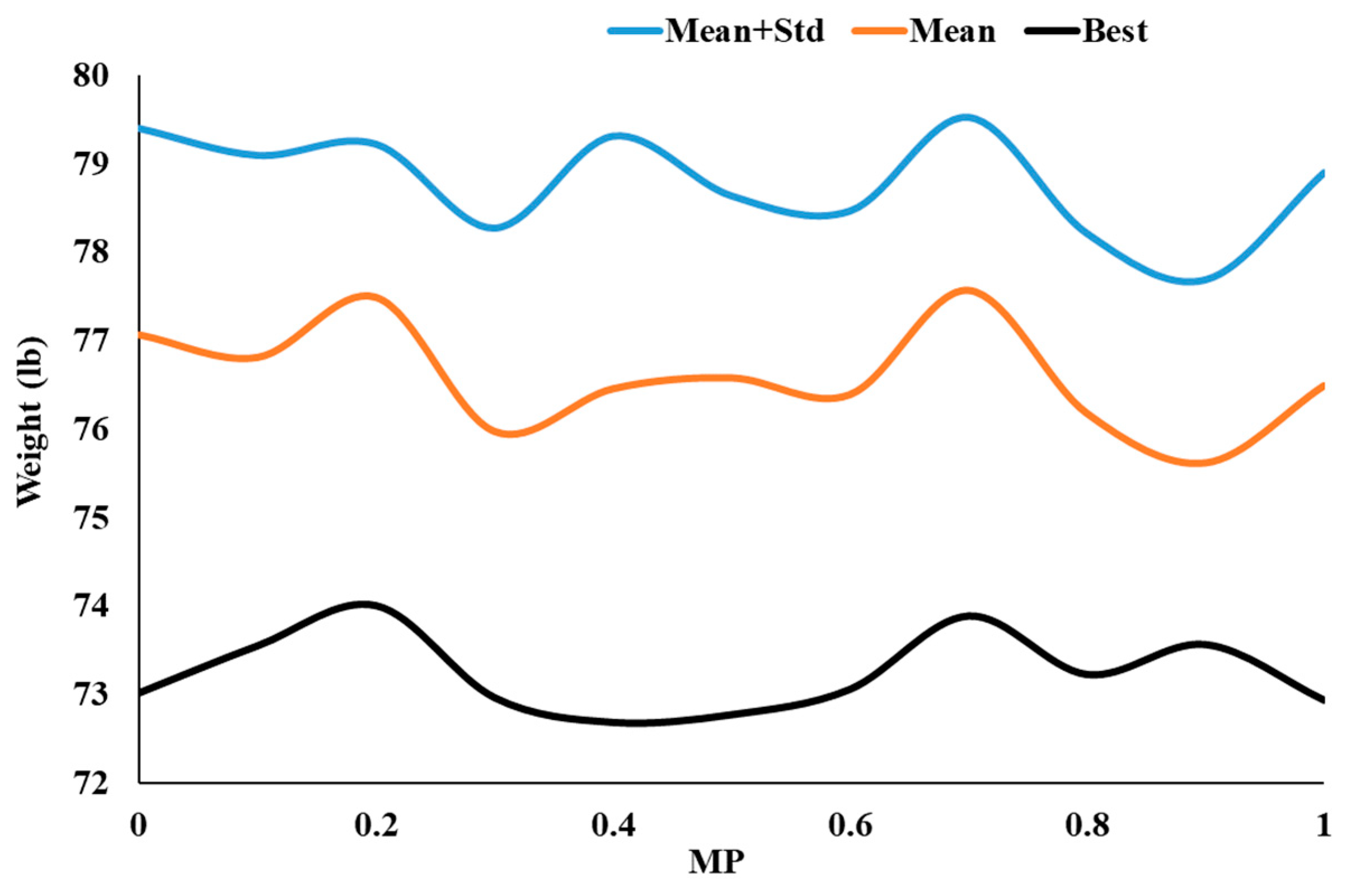
| MP | 0 | 0.1 | 0.2 | 0.3 | 0.4 | 0.5 | 0.6 | 0.7 | 0.8 | 0.9 | 1 |
|---|---|---|---|---|---|---|---|---|---|---|---|
| Best weight (lb) | 73.013 | 73.544 | 73.996 | 72.959 | 72.681 | 72.768 | 73.053 | 73.880 | 73.220 | 73.558 | 72.933 |
| Mean (lb) | 77.063 | 76.808 | 77.484 | 75.975 | 76.456 | 76.578 | 76.389 | 77.562 | 76.179 | 75.622 | 76.489 |
| Std (lb) | 2.331 | 2.281 | 1.731 | 2.294 | 2.850 | 2.055 | 2.073 | 1.956 | 2.031 | 2.065 | 2.403 |
| Mean + Std (lb) | 79.394 | 79.089 | 79.215 | 78.270 | 79.306 | 78.633 | 78.463 | 79.519 | 78.210 | 77.687 | 78.892 |
| No. | Design Variables | GA [54] | ARSAGA [55] | SCPSO [56] | IGA [57] | FA [58] | TLBO [59] | MHS [60] | D-ICDE [61] | ABC [62] | MLA [63] | CSBO | NCSBO |
|---|---|---|---|---|---|---|---|---|---|---|---|---|---|
| 1 | A1 | 1.081 | 0.954 | 0.954 | 1.081 | 0.954 | 1.081 | 0.954 | 1.081 | 0.954 | 0.954 | 0.954 | 0.954 |
| 2 | A2 | 0.539 | 1.081 | 0.539 | 0.539 | 0.539 | 0.954 | 0.539 | 0.539 | 0.539 | 0.539 | 0.539 | 0.539 |
| 3 | A3 | 0.287 | 0.44 | 0.27 | 0.287 | 0.22 | 0.141 | 0.22 | 0.141 | 0.347 | 0.347 | 0.141 | 0.174 |
| 4 | A4 | 0.954 | 1.174 | 0.954 | 0.954 | 0.954 | 1.081 | 0.954 | 0.954 | 0.954 | 0.954 | 0.954 | 0.954 |
| 5 | A5 | 0.539 | 1.488 | 0.539 | 0.954 | 0.539 | 0.539 | 0.539 | 0.539 | 0.539 | 0.539 | 0.539 | 0.539 |
| 6 | A6 | 0.141 | 0.27 | 0.174 | 0.22 | 0.22 | 0.347 | 0.22 | 0.287 | 0.111 | 0.111 | 0.27 | 0.27 |
| 7 | A7 | 0.111 | 0.27 | 0.111 | 0.111 | 0.111 | 0.111 | 0.111 | 0.111 | 0.111 | 0.111 | 0.111 | 0.111 |
| 8 | A8 | 0.111 | 0.347 | 0.111 | 0.111 | 0.111 | 0.174 | 0.111 | 0.111 | 0.111 | 0.111 | 0.111 | 0.111 |
| 9 | A9 | 0.539 | 0.22 | 0.287 | 0.287 | 0.287 | 0.141 | 0.44 | 0.141 | 0.539 | 0.347 | 0.539 | 0.347 |
| 10 | A10 | 0.44 | 0.44 | 0.347 | 0.22 | 0.44 | 0.27 | 0.347 | 0.347 | 0.44 | 0.44 | 0.347 | 0.347 |
| 11 | A11 | 0.539 | 0.22 | 0.347 | 0.44 | 0.44 | 0.22 | 0.347 | 0.440 | 0.44 | 0.44 | 0.347 | 0.347 |
| 12 | A12 | 0.27 | 0.44 | 0.22 | 0.44 | 0.22 | 0.141 | 0.27 | 0.270 | 0.174 | 0.174 | 0.27 | 0.22 |
| 13 | A13 | 0.22 | 0.347 | 0.22 | 0.111 | 0.22 | 0.44 | 0.27 | 0.270 | 0.174 | 0.174 | 0.22 | 0.22 |
| 14 | A14 | 0.141 | 0.27 | 0.174 | 0.22 | 0.27 | 0.347 | 0.22 | 0.287 | 0.111 | 0.111 | 0.27 | 0.27 |
| 15 | A15 | 0.287 | 0.22 | 0.27 | 0.347 | 0.22 | 0.141 | 0.22 | 0.174 | 0.347 | 0.347 | 0.141 | 0.174 |
| 16 | X2 | 101.5775 | 118.346 | 137.2216 | 133.612 | 114.967 | 100.004 | 135.568 | 100.0309 | 110.209 | 108.1889 | 133.213 | 133.9027 |
| 17 | X3 | 227.9112 | 225.209 | 259.9093 | 234.752 | 247.04 | 241.047 | 245.542 | 238.7010 | 249.819 | 246.2332 | 257.87 | 259.7541 |
| 18 | Y2 | 134.7986 | 119.046 | 123.5006 | 100.449 | 125.919 | 118.823 | 123.13 | 132.8471 | 133.599 | 135.0565 | 118.672 | 120.6040 |
| 19 | Y3 | 128.2206 | 105.086 | 110.002 | 104.738 | 111.067 | 100.083 | 120.696 | 125.3669 | 111.624 | 113.7962 | 111.769 | 106.7233 |
| 20 | Y4 | 54.863 | 63.375 | 59.9356 | 73.762 | 58.298 | 50 | 57.9313 | 60.3072 | 55.1278 | 55.4635 | 53.0239 | 51.0915 |
| 21 | Y6 | −16.4484 | −20 | −5.1799 | −10.067 | −17.564 | 3.1411 | −5.9742 | −10.6651 | −18.950 | 18.0985 | −11.965 | −9.57978 |
| 22 | Y7 | −16.4484 | −20 | 4.2193 | −1.339 | −5.821 | −9.6997 | −2.9125 | −12.2457 | 3.3411 | 1.9869 | −5.4549 | 0.67778 |
| 23 | Y8 | 54.8572 | 57.722 | 57.8829 | 50.402 | 31.465 | 46.8963 | 56.3256 | 59.9931 | 55.1423 | 55.4635 | 53.0262 | 51.2169 |
| Best weight (lb) | 76.6854 | 104.573 | 72.5143 | 79.82 | 75.55 | 76.6519 | 73.887 | 74.6818 | 72.715 | 72.478 | 72.66 | 72.224 [72.5143] b [73.887] c | |
| Mean weight (lb) | N/A a | N/A | 76.411 | N/A | N/A | N/A | N/A | N/A | 77.2558 | 75.2119 | 76.83 | 76.37 | |
| Worst weight (lb) | N/A | N/A | 80.156 | N/A | N/A | N/A | N/A | N/A | 78.9446 | 78.6951 | 79.683 | 78.98 | |
| ODNSA | N/A | N/A | 4500 | 8000 | 8000 | 30,640 | 5000 | 7980 | 5640 | 30,000 | 7620 | 5430 | |
| TNSA | N/A | N/A | 4500 | 8000 | 8000 | 32,000 | 5000 | 7980 | 18,000 | 30,000 | 18,000 | 18,000 | |
| STD (lb) | N/A | N/A | 1.922 | N/A | N/A | N/A | N/A | N/A | 2.4219 | 1.8314 | 2.482 | 1.73 | |
| CVP (%) | None | 32.57 | 0 | 0.00089 | None | None | None | None | None | None | None | None | |
| No. | Design Variables | SCPSO [56] | VGA [64] | GA [65] | GSO [66] | IGSO [66] | D-ICDE [61] | ABC [62] | MLA [63] | CSBO | NCSBO |
|---|---|---|---|---|---|---|---|---|---|---|---|
| 1 | G1 | 12.5 | 12.5 | 12.25 | 12.25 | 12.25 | 13 | 12.5 | 9.75 | 12.50 | 12.5 |
| 2 | G2 | 17.5 | 16.25 | 18 | 18.25 | 18.25 | 17.5 | 17.75 | 18.75 | 17.50 | 17.5 |
| 3 | G3 | 5.75 | 8 | 5.25 | 4.75 | 4.75 | 6.5 | 5.75 | 5.5 | 6.00 | 5.75 |
| 4 | G4 | 3.75 | 4 | 4.25 | 4.25 | 4.25 | 3 | 3.75 | 3.5 | 3.75 | 3.75 |
| 5 | X3 | 907.2491 | 891.9 | 913 | 916.9 | 920.812 | 914.06 | 912.997 | 931.4057 | 906.747 | 907.7788 |
| 6 | Y3 | 179.8671 | 145.3 | 186.8 | 191.971 | 170.912 | 183.46 | 183.681 | 187.5341 | 179.523 | 180.4711759 |
| 7 | X5 | 636.7873 | 610.6 | 650 | 654.224 | 640.506 | 640.53 | 642.714 | 662.7803 | 635.496 | 637.3638803 |
| 8 | Y5 | 141.8271 | 118.2 | 150.5 | 156.1 | 139.87 | 133.74 | 143.892 | 162.0359 | 139.864 | 141.3239515 |
| 9 | X7 | 407.9442 | 385.4 | 418.8 | 423.5 | 409.416 | 406.12 | 411.692 | 427.3530 | 406.841 | 408.0822344 |
| 10 | Y7 | 94.0559 | 72.5 | 97.4 | 102.571 | 91.774 | 92.63 | 97.1476 | 99.4025 | 95.461 | 93.88007802 |
| 11 | X9 | 198.7897 | 184.4 | 204.8 | 207.519 | 198.775 | 196.69 | 200.909 | 210.1569 | 198.719 | 198.7942297 |
| 12 | Y9 | 29.5157 | 23.4 | 26.7 | 28.579 | 29.504 | 37.06 | 30.2191 | 28.3101 | 29.457 | 29.51760031 |
| Best weight (lb) | 4512.365 | 4616.8 | 4547.9 | 4538.7676 | 4553.12 | 4554.29 | 4537.06 | 4271.57 | 4530.13 | 4512.1244 [4537.06] a | |
| Mean weight (lb) | 4551.709 | N/A | N/A | N/A | N/A | N/A | 4585.110 | 4317.984 | 4539.63 | 4534.3 | |
| Worst weight (lb) | 4661.268 | N/A | N/A | N/A | N/A | N/A | 4627.524 | 4348.598 | 4553.22 | 4548.19 | |
| ODNSA | 4500 | N/A | N/A | 50,000 | 50,000 | 8025 | 2700 | 30,000 | 7585 | 5900 | |
| TNSA | 4500 | N/A | N/A | 50,000 | 50,000 | 8025 | 18,000 | 30,000 | 18,000 | 18,000 | |
| STD (lb) | 37.69 | N/A | N/A | N/A | N/A | N/A | 9.797 | 24.769 | 5.73 | 5.38 | |
| CVP (%) | 0 | 0.0079 | None | None | 94.28 | None | None | 24.87 | None | None | |
| No. | Design Variables | SCPSO [56] | GA [65] | GA [57] | MHS [60] | FA [58] | D-ICDE [61] | ABC [62] | MLA [63] | CSBO | NCSBO |
|---|---|---|---|---|---|---|---|---|---|---|---|
| 1 | A1 (in2) | 0.1 | 0.1 | 0.1 | 0.1 | 0.1 | 0.1 | 0.1 | 0.1 | 0.1 | 0.1 |
| 2 | A2 | 0.1 | 0.1 | 0.1 | 0.1 | 0.1 | 0.1 | 0.1 | 0.1 | 0.1 | 0.1 |
| 3 | A3 | 1 | 1.1 | 1.1 | 1 | 1 | 0.9 | 1 | 1.0 | 1 | 1 |
| 4 | A4 | 0.1 | 0.1 | 0.1 | 0.1 | 0.1 | 0.1 | 0.1 | 0.1 | 0.1 | 0.1 |
| 5 | A5 | 0.1 | 0.1 | 0.1 | 0.1 | 0.1 | 0.1 | 0.1 | 0.1 | 0.1 | 0.1 |
| 6 | A6 | 0.1 | 0.1 | 0.2 | 0.1 | 0.1 | 0.1 | 0.1 | 0.1 | 0.1 | 0.1 |
| 7 | A7 | 0.1 | 0.1 | 0.2 | 0.1 | 0.1 | 0.1 | 0.1 | 0.1 | 0.1 | 0.1 |
| 8 | A8 | 0.9 | 1 | 0.7 | 1 | 1 | 1.0 | 0.9 | 0.9 | 0.9 | 0.9 |
| 9 | X4 (in) | 36.952 | 36.230 | 35.470 | 37.820 | 37.320 | 36.830 | 36.211 | 37.759 | 37.498 | 37.67668 |
| 10 | Y4 | 54.5786 | 58.560 | 60.370 | 55.485 | 55.740 | 58.530 | 54.637 | 54.625 | 54.672 | 54.50722 |
| 11 | Z4 | 129.9758 | 115.590 | 129.070 | 128.730 | 126.620 | 122.670 | 129.965 | 129.625 | 130 | 130 |
| 12 | X8 | 51.7317 | 46.460 | 45.060 | 52.068 | 50.140 | 49.210 | 52.074 | 51.927 | 51.880 | 51.87948 |
| 13 | Y8 | 139.5316 | 127.950 | 137.040 | 139.590 | 136.400 | 136.740 | 139.980 | 139.678 | 139.494 | 139.5099 |
| Best weight (lb) | 117.227 | 124.0015 | 124.940 | 117.380 | 118.830 | 118.760 | 117.333 | 117.316 | 117.264 | 117.257 | |
| Mean weight (lb) | 122.876 | N/A | N/A | N/A | N/A | N/A | N/A | 123.728 | 119.702 | 117.336 | |
| Worst weight (lb) | 132.672 | N/A | N/A | N/A | N/A | N/A | N/A | 127.482 | 124.665 | 117.647 | |
| ODNSA | 4500 | N/A | 6000 | 6000 | 6000 | 6000 | 5100 | 30,000 | 5310 | 4830 | |
| TNSA | 4500 | N/A | 6000 | 6000 | 6000 | 6000 | 18,000 | 30,000 | 18,000 | 18,000 | |
| STD (lb) | 3.671 | N/A | N/A | N/A | N/A | N/A | 2.22 | 2.384 | 0.352 | 0.142 | |
| CVP (%) | 0.527 | None | 0.008 | None | None | 0.17 | None | None | None | None | |
| No. | Design Variables | SCPSO [56] | BBM [67] | GA [68] | D-ICDE [61] | ABC [62] | MLA [63] | CSBO | NCSBO |
|---|---|---|---|---|---|---|---|---|---|
| 1 | A1 (in2) | 2.5 | 2.7 | 2.5 | 2.7 | 2.4 | 2.7 | 2.9 | 2.8 |
| 2 | A2 | 2.5 | 2.6 | 2.2 | 3 | 2.2 | 2.5 | 2.6 | 2.6 |
| 3 | A3 | 0.8 | 0.7 | 0.7 | 0.5 | 1.1 | 0.7 | 0.6 | 0.7 |
| 4 | A4 | 0.1 | 0.4 | 0.1 | 1.1 | 0.1 | 0.1 | 0.1 | 0.1 |
| 5 | A5 | 0.7 | 0.8 | 1.3 | 0.7 | 1.2 | 1 | 1 | 0.9 |
| 6 | A6 | 1.4 | 1.2 | 1.3 | 1.5 | 1.3 | 1.3 | 1.1 | 1.1 |
| 7 | A7 | 1.7 | 1.7 | 1.8 | 2.1 | 1.7 | 2 | 2 | 2 |
| 8 | A8 | 0.8 | 0.8 | 0.5 | 0.9 | 0.6 | 0.6 | 0.6 | 0.6 |
| 9 | A9 | 0.9 | 1.1 | 0.8 | 0.8 | 0.8 | 0.9 | 0.9 | 0.9 |
| 10 | A10 | 1.3 | 1.4 | 1.2 | 1.8 | 1.6 | 1.4 | 1.3 | 1.3 |
| 11 | A11 | 0.3 | 0.4 | 0.4 | 0.4 | 0.3 | 0.3 | 0.5 | 0.5 |
| 12 | A12 | 0.9 | 1 | 1.2 | 1 | 0.9 | 1.1 | 1.3 | 1.3 |
| 13 | A13 | 1 | 1 | 0.9 | 1.3 | 1.2 | 1.1 | 1 | 1 |
| 14 | A14 | 1.1 | 1.1 | 1 | 1.6 | 1 | 1.1 | 1 | 1 |
| 15 | A15 | 5 | 0.8 | 3.6 | 1 | 1 | 0.9 | 0.7 | 0.7 |
| 16 | A16 | 0.1 | 0.6 | 0.1 | 0.4 | 0.6 | 0.1 | 0.1 | 0.1 |
| 17 | A17 | 2.5 | 2.7 | 2.4 | 3 | 2.8 | 2.6 | 2.8 | 2.8 |
| 18 | A18 | 1 | 0.9 | 1.1 | 0.9 | 0.4 | 1 | 0.9 | 0.8 |
| 19 | A19 | 0.1 | 0.1 | 0.1 | 0.2 | 0.1 | 0.1 | 0.1 | 0.1 |
| 20 | A20 | 2.8 | 2.9 | 2.7 | 3.3 | 2.9 | 2.9 | 3 | 3 |
| 21 | A21 | 0.9 | 1 | 0.8 | 0.4 | 1.5 | 0.8 | 0.9 | 0.8 |
| 22 | A22 | 0.1 | 0.5 | 0.1 | 0.1 | 0.6 | 0.1 | 0.1 | 0.1 |
| 23 | A23 | 3 | 3.1 | 2.8 | 3.3 | 3.1 | 3.1 | 3.1 | 3.1 |
| 24 | A24 | 1 | 1.1 | 1.3 | 0.3 | 0.9 | 1 | 1 | 1 |
| 25 | A25 | 0.1 | 0.1 | 0.2 | 0.1 | 0.1 | 0.1 | 0.1 | 0.1 |
| 26 | A26 | 3.2 | 3.2 | 3 | 3.3 | 3.3 | 3.2 | 3.2 | 3.2 |
| 27 | A27 | 1.2 | 1.1 | 1.2 | 0.5 | 0.8 | 1.3 | 1.2 | 1.2 |
| 28 | X2 (in) | 101.3393 | 106 | 114 | 106.2986 | 103.6063 | 104.929 | 102.916 | 103.16734 |
| 29 | X4 | 85.9111 | 89 | 97 | 82.4936 | 81.5008 | 78.2568 | 83.58044 | 83.31772 |
| 30 | Y4 | 135.9645 | 136 | 125 | 136.9634 | 143.0525 | 156.6791 | 150.4427 | 148.59871 |
| 31 | X6 | 74.7969 | 66 | 76 | 62.7192 | 67.0169 | 67.7817 | 64.41907 | 65.00997 |
| 32 | Y6 | 237.7447 | 255 | 261 | 244.4495 | 252.8466 | 254.8397 | 263.1986 | 261.78296 |
| 33 | X8 | 64.3115 | 57 | 69 | 47.563 | 54.5203 | 59.7804 | 53.52898 | 54.22948 |
| 34 | Y8 | 321.3416 | 342 | 316 | 332.7201 | 374.0126 | 323.7404 | 333.5202 | 329.84055 |
| 35 | X10 | 53.3345 | 50 | 56 | 42.7377 | 39.8226 | 50.386 | 46.75877 | 47.56234 |
| 36 | Y10 | 414.3025 | 415 | 414 | 401.7876 | 443.9461 | 414.8346 | 398.9399 | 398.27862 |
| 37 | X12 | 46.0277 | 45 | 50 | 32.8229 | 30.9474 | 42.9782 | 42.57715 | 43.52248 |
| 38 | Y12 | 489.9216 | 475 | 463 | 468.0985 | 491.9941 | 467.3015 | 445.722 | 450.88035 |
| 39 | X14 | 41.8353 | 40 | 54 | 27.0026 | 36.7597 | 43.9541 | 44.47806 | 43.90031 |
| 40 | Y14 | 522.4161 | 513 | 524 | 500.416 | 510 | 516.8386 | 497.4669 | 494.24315 |
| 41 | X20 | 1.0005 | 17 | 1 | 11.9079 | 17.6763 | 12.2461 | 1.639016 | 2.05889 |
| 42 | Y20 | 598.3905 | 598 | 587 | 581.5046 | 598.8911 | 586.3233 | 571.3341 | 571.56796 |
| 43 | X21 | 97.8696 | 93 | 99 | 82.6543 | 77.6661 | 91.1605 | 86.42174 | 86.39172 |
| 44 | Y21 | 624.0552 | 624 | 631 | 611.0089 | 619.8911 | 621.2209 | 629.3503 | 629.35088 |
| Best weight (lb) | 1864.10 | 1934.17 | 1925.79 | 1744.8 | 1871.843 | 1888.146 | 1881.965 | 1864.7753 | |
| Mean weight (lb) | 1894.056 | N/A | N/A | N/A | 1887.838 | 1912.530 | 1909.574 | 1891.056 | |
| Worst weight (lb) | 2007.563 | N/A | N/A | N/A | 1961.119 | 1929.989 | 1962.741 | 1918.475 | |
| ODNSA | 25,000 | N/A | 100,000 | 17,745 | 2850 | 30,000 | 8910 | 7590 | |
| TNSA | 25,000 | N/A | 100,000 | 17,745 | 18,000 | 30,000 | 18,000 | 18,000 | |
| STD (lb) | 34.755 | N/A | N/A | N/A | 7.5649 | 11.534 | 25.38 | 15.47 | |
| CVP (%) | 0 | 0.201 | 0 | 966.92 | 269.77 | 0 | 0 | 0 | |
Disclaimer/Publisher’s Note: The statements, opinions and data contained in all publications are solely those of the individual author(s) and contributor(s) and not of MDPI and/or the editor(s). MDPI and/or the editor(s) disclaim responsibility for any injury to people or property resulting from any ideas, methods, instructions or products referred to in the content. |
© 2025 by the authors. Licensee MDPI, Basel, Switzerland. This article is an open access article distributed under the terms and conditions of the Creative Commons Attribution (CC BY) license (https://creativecommons.org/licenses/by/4.0/).
Share and Cite
Ugur, I.B.; Degertekin, S.O. A New Approach to Circulatory System-Based Optimization for the Shape and Sizing Design of Truss Structures. Appl. Sci. 2025, 15, 3671. https://doi.org/10.3390/app15073671
Ugur IB, Degertekin SO. A New Approach to Circulatory System-Based Optimization for the Shape and Sizing Design of Truss Structures. Applied Sciences. 2025; 15(7):3671. https://doi.org/10.3390/app15073671
Chicago/Turabian StyleUgur, Ibrahim Behram, and Sadik Ozgur Degertekin. 2025. "A New Approach to Circulatory System-Based Optimization for the Shape and Sizing Design of Truss Structures" Applied Sciences 15, no. 7: 3671. https://doi.org/10.3390/app15073671
APA StyleUgur, I. B., & Degertekin, S. O. (2025). A New Approach to Circulatory System-Based Optimization for the Shape and Sizing Design of Truss Structures. Applied Sciences, 15(7), 3671. https://doi.org/10.3390/app15073671