Accurate Rotor Temperature Prediction of Permanent Magnet Synchronous Motor in Electric Vehicles Using a Hybrid RIME-XGBoost Model

Abstract

With the growing global focus on environmental protection and carbon emissions, electric vehicles (EVs) are becoming increasingly popular. Permanent magnet synchronous motors (PMSMs) have emerged as a core component of the drive system due to their high-power density and compact design. The rotor temperature of PMSMs significantly affects their operating efficiency, management strategies, and lifespan. However, real-time monitoring and acquisition of rotor temperature are challenging due to cost and space limitations. Therefore, this study proposes a hybrid model named RIME-XGBoost, which integrates the RIME optimization algorithm with XGBoost, for the precise modeling and prediction of PMSM rotor temperature. RIME-XGBoost utilizes easily monitored dynamic parameters such as motor speed, torque, and currents and voltages in the d-q coordinate system as input features. It simultaneously optimizes three hyperparameters (number of trees, tree depth, and learning rate) to achieve high learning efficiency and good generalization performance. The experimental results show that, on both medium-scale datasets and small-sample datasets in high-temperature ranges, RIME-XGBoost outperforms existing methods such as SMA-RF, SO-BiGRU, and EO-SVR in terms of RMSE, MBE, R-squared, and Runtime. RIME-XGBoost effectively enhances the prediction accuracy and computational efficiency of rotor temperature. This study provides a new technical solution for temperature management in EVs and offers valuable insights for research in related fields.

1. Introduction

The global push for environmental sustainability has positioned electric vehicles (EVs) as crucial solutions for carbon reduction [1,2,3,4]. The preferred EV propulsion technology is permanent magnet synchronous motors (PMSMs) due to their high power density and compact design [5,6,7]. Thermal behavior fundamentally determines PMSMs’ performance [8], directly impacting operational efficiency and component longevity. This transition elevates the importance of thermal management for PMSMs.

Real-world EV operation subjects the rotors in PMSMs to significant thermal stress from dynamic driving conditions: frequent torque variations, sudden load changes, and diverse terrain demands [9]. These fluctuations create critical reliability challenges through two primary mechanisms: temperature-dependent demagnetization of permanent magnets and thermal degradation of electromagnetic properties in structural materials [10]. Effective thermal modeling of rotors thus becomes essential for maintaining both the efficiency and operational safety of PMSMs under practical driving scenarios.

Direct rotor temperature measurement in PMSMs faces inherent limitations, including complex sensor integration and spatial constraints [11,12]. The temperature-dependent variation in motor parameters (e.g., rotor resistance, magnetizing inductance) introduces additional control complexity under variable loads [13]. This makes accurate thermal modeling particularly challenging.

Model-based prediction methods have become increasingly adopted for PMSMs’ thermal management [14]. Kang et al. [15] modified the lumped-parameter model by incorporating rotor slot cooling dynamics. They improved predictions of air velocity and temperature distribution. Song et al. [16] introduced segmented stator shell modules (PSMs) and developed an LPTN model that achieves better temperature prediction accuracy under braking system failure conditions. Some advances combine Finite Element Analysis (FEA) with thermal modeling for improved prediction. Pereira and Rui Esteves Araújo [17] developed a model-free predictive current control method enabling low-computation parameter identification. Kumar et al. [18] integrated signal processing with image analysis to correlate temperature data with rotor slot changes. Hybrid modeling approaches also show particular promise. Ye et al. [19] combined 2D/3D thermal networks for speed-dependent temperature prediction, while Zhou et al. [20] enhanced computational efficiency through intelligent grid classification in magnetic–thermal field analysis. Innovations in thermal modeling encompass multiple approaches. Bouziane et al. [21] introduced a Bidirectional LSTM (Bi-LSTM) architecture specifically designed for capturing nonlinear parameter correlations. Hu et al. established temperature trends through combined loss analysis and cooling dynamics [14], while Cuiping et al. created a 3D transient model for micro EV induction motors using time-stepping Finite Element Methods (FEMs) [22]. Pandey et al. [8] achieved enhanced prediction accuracy through reformulated RANS equations.

While these methods demonstrate progress, critical limitations persist. Simplified models often sacrifice accuracy for speed, while loss-based estimations accumulate error propagation. Traditional FEA remains computationally intensive and data-demanding. FEMs offer computational advantages but risk instability with improper meshing.

Complementing these physical models, machine learning approaches show growing potential [23]. Recent studies have explored data-driven approaches for rotor temperature prediction, demonstrating their advantages over traditional physics-based methods like Linear Parameterized Thermal Network (LPTN) models. Kirchgässner et al. [24] compared machine learning models against LPTNs. Their results showed that ordinary least squares (OLSs) and shallow MLPs achieved comparable accuracy with minimal computational complexity. Zhang et al. [25] leveraged a modified transformer-based model (MT-LSTR) which was trained on simulated data to predict temperature dynamics effectively. Meanwhile, Jing et al. [26,27] proposed two distinct data-driven strategies: a Gradient Boosting Decision Tree (GBDT) ensemble to model nonlinear relationships between stator and rotor temperatures and a model-free SVR method with a linear kernel. This study reduced reliance on domain expertise while reliably estimating temperatures.

XGBoost (eXtreme Gradient Boosting, version 1.7.0) is a powerful machine learning method that has gained attention in engineering applications for optimizing systems and improving predictions [28,29]. Recent research has further demonstrated its versatility. Jin et al. [30] developed an AI-Enabled Energy-Saving Strategy (AIESS) combining XGBoost and Genetic Algorithms (GAs) to minimize energy consumption in electro-hydraulic systems. Similarly, Li et al. [31] employed XGBoost to enhance photovoltaic power generation forecasting, leveraging its ability to handle nonlinear relationships between environmental variables and energy generation. Pan and Fang [32] integrated XGBoost with FEA to refine torque characteristics, predict torque ripple, and adjust operational parameters. Lin et al. [33] advanced temperature prediction using XGBoost. Their method integrated data normalization, Bayesian hyperparameter optimization, and model training. Shimizu et al. [34,35] further extended XGBoost’s utility in sustainable motor design by developing surrogate models to accelerate the optimization of interior PMSMs. Collectively, these studies highlight the potential of machine learning (particularly XGBoost) to enhance precision, reduce computational demands, and adapt to dynamic thermal conditions in PMSMs.

While existing methods address specific operational scenarios, three critical limitations persist under complex driving conditions: (1) insufficient generalization, (2) accuracy–computation efficiency tradeoffs, and (3) limited real-time adaptability.

This study proposes a novel hybrid method combining machine learning and metaheuristic algorithms to establish a prediction model for the rotor temperature of PMSMs. The model is based on XGBoost and optimizes three hyperparameters (number of trees, tree depth, and learning rate) using the RIME (Rime optimization algorithm). By adaptively enhancing XGBoost according to the data scale and input samples, a hybrid model with high learning ability and generalization capability is established, named RIME-XGBoost. The input features for modeling include easily monitored variables of the PMSM, such as motor speed, torque, currents, and voltages in the d/q coordinate system, with rotor temperature as the target variable. Prediction experiments are conducted using these features. To test the characteristics and applicability of the developed model, experiments are carried out using medium-scale data with large temperature fluctuations and small-sample data collected in high-temperature ranges. For comparison, three recently published hybrid models are selected, i.e., Random Forest (RF) optimized by the Slime Mould Algorithm (SMA), BiGRU optimized by the Snake Optimizer (SO), and Support Vector Regression (SVR) optimized by the Equilibrium Optimizer (EO). The prediction accuracy, stability, and computational efficiency of each model are evaluated using metrics such as Root Mean Square Error (RMSE), Mean Bias Error (MBE), R-squared, and Runtime.

This article is organized as follows. Section 2 describes the source, composition, and processing of the experimental data. Section 3 introduces the basic theories of XGBoost and RIME. Section 4 presents the various hybrid models used for comparison and describes the metrics for quantifying the test results. Section 5 investigates the effectiveness and characteristics of RIME-XGBoost using medium-scale and small-scale samples and provides a detailed discussion with the comparison models. Subsequently, the reasons for the excellent performance of RIME-XGBoost are analyzed. Finally, the conclusions and future work of this paper are summarized.

2. Data and Their Processing

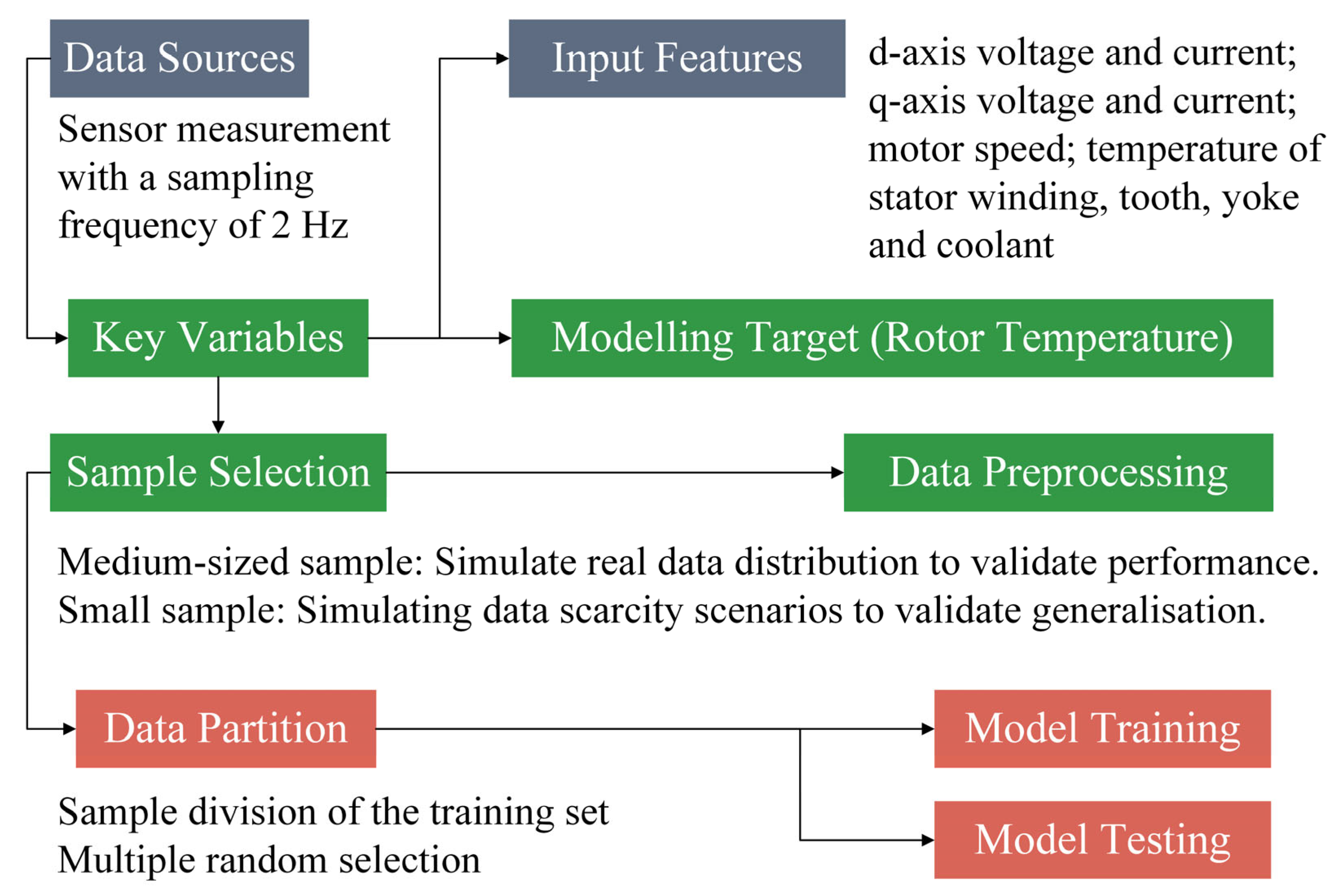
2.1. Data Sources and Composition

The dataset used in this study is named “Electric Motor Temperature”, collected and released by the LEA Laboratory at Paderborn University, Paderborn, Germany [36]. The experimental data were measured directly from a test bench equipped with a 52 kW three-phase automotive traction PMSM. The measurement setup includes the following [36]:

(1) Thermocouples (type K, class 1) embedded in the stator teeth, winding, yoke, and rotor permanent magnets.

(2) A telemetry unit to transmit rotor temperature data (average of four permanent magnet surface sensors).

(3) dSPACE DS1006MC rapid control prototyping system (dSPACE, Paderborn, Germany) and analog–digital converters (ADCs) for synchronized data acquisition.

(4) All signals were sampled at 2 Hz over 140 h of operation.

(5) Preprocessing steps, including exponentially weighted moving averages (EWMAs) and standard deviations (EWMS), were applied to enhance regression features.

The dataset explicitly reflects real-world PMSM dynamics. Thus, the training of the proposed model on empirical data from a physical test bench ensures alignment with actual thermal behavior. The test bench for the PMSM is shown in Figure 1.

The dataset is organized in a tabular format, with each record (sample) representing sensor measurements at a specific time point. The dataset includes multiple measurement sessions (sample numbers), and the main variables are listed in

Table 1. Key variables and descriptions in each sample.

Variable Type	Variable	Description
Input Feature	u_q	The q-axis component of the voltage measured in the dq-coordinate system
	coolant	The temperature of the coolant
	stator_winding	The temperature of the stator windings
	u_d	The d-axis component of the voltage
	stator_tooth	The temperature of the stator teeth
	motor_speed	The rotational speed of the motor
	i_d	The d-axis component of the current
	i_q	The q-axis component of the current
	stator_yoke	The temperature of the stator yoke
Target	pm	The temperature of the permanent magnet

.

These input features can be categorized into four types. The motor speed and torque are motor state variables. Currents (i_d, i_q) and voltages (u_d, u_q) in the d/q coordinate system are also motor state variables. Temperature variables include pm (permanent magnet temperature) and stator_yoke. However, pm is difficult to monitor, while stator_yoke is relatively easy to monitor. Therefore, pm is chosen as the modeling target, while the other variables serve as modeling features.

2.2. Data Processing and Utilization

The dataset includes multiple experiments, each with varying motor temperature ranges. By traversing the dataset, it was found that group number 24 (hereafter referred to as Group A) has the largest range of motor rotor temperature variation, with a minimum value of 21.93 °C and a maximum value of 113.61 °C. Group number 46 (hereafter referred to as Group B) has the fewest samples, and the motor rotor temperatures are concentrated in the high-temperature range, with a minimum value of 78.08 °C and a maximum value of 92.91 °C.

Table 2. The rotor temperature range and sample size of each group.

No.	Range	Count	No.	Range	Count	No.	Range	Count
2	23.02	19,357	27	87.41	35,361	59	47.07	7475
3	6.26	19,248	29	75.60	21,358	60	49.64	14,543
4	76.47	33,424	30	30.39	23,863	61	31.82	14,516
5	14.05	14,788	31	78.07	15,587	62	53.21	25,600
6	69.16	40,388	32	67.13	20,960	63	44.21	16,668
7	10.79	14,651	36	26.01	22,609	64	43.03	6250
8	20.27	18,757	41	67.85	16,700	65	67.39	40,094
9	26.31	20,336	42	45.88	16,920	66	44.58	36,476
10	49.15	15,256	43	41.02	8443	67	39.69	11,135
11	32.88	7887	44	51.75	26,341	68	58.01	23,331
12	23.76	21,942	45	63.36	17,142	69	59.07	15,350
13	10.85	35,906	46	14.83	2180	70	42.50	25,677
14	36.00	18,598	48	33.44	21,983	71	54.60	14,656
15	72.79	18,124	49	42.17	10,816	72	41.07	15,301
16	23.15	20,645	50	41.19	10,810	73	63.41	16,786
17	45.32	15,964	51	52.88	6261	74	29.04	23,761
18	15.39	37,732	52	28.76	3726	75	70.31	13,472
19	72.31	10,410	53	37.90	32,442	76	51.12	22,188
20	82.41	43,971	54	47.44	10,807	78	46.76	8445
21	70.65	17,321	55	52.71	10,807	79	71.60	31,154
23	74.11	11,856	56	43.60	33,123	80	58.49	23,824
24	91.67	15,015	57	62.35	14,403	81	52.65	17,672
26	71.56	16,666	58	54.84	33,382	/	/	/

records the variation range of the rotor temperature and the total sample size.

These two groups were selected for further study. The focus is on establishing a mapping model, with rotor temperature as the prediction target and the other variables as inputs. Different preprocessing methods were applied to Groups A and B. Data description, preprocessing, and usage are illustrated in Figure 2.

Group A contains 15,015 samples. A preprocessing method was used where every fifth sample was retained, resulting in a moderately sized dataset of 3003 samples. Given the original sampling frequency of 2 Hz, the time interval between data points is short, meaning adjacent samples have highly similar information. Since the primary goal is to predict rotor temperature, which typically does not change rapidly, a very high sampling frequency is unnecessary for analyzing its dynamics. This preprocessing method effectively reduces data redundancy while retaining sufficient information for modeling and analysis. Subsequently, 500 samples were randomly selected as the training set, and the remaining samples formed the test set. Compared to the typical 7:3 ratio, this approach allows the test set to better simulate the distribution of unknown data, providing a more realistic assessment of the model’s performance in practical applications.

Group B follows a similar approach. From a total of 2180 samples, every 10th sample was retained, resulting in a new dataset of 218 samples. This small sample size effectively tests the model’s generalization ability under limited data conditions. If the model performs well, this indicates a strong learning capability and can achieve high prediction accuracy even with scarce data. In practical applications, large quantity data acquisition may be of great difficulty, e.g., requires a high cost, under certain rotor temperature scenarios. Therefore, Group B aims to simulate these scenarios and test the model’s performance. The ratio of the training set to the test set is 1:1, meaning that half of the data are randomly selected for training, and the rest are used to test the model’s generalization ability.

The data (Group A and B) and their description can be found at the following URL (accessed on 18 February 2025): https://github.com/567ZYC/Data-Explanation-for-Electric-Motor-Temperature-Dataset.

2.3. The Impact of Data Preprocessing on Model Performance

EWMAs and EWMS are applied to smooth the time-series data, which likely reduces high-frequency noise inherent in sensor measurements. They can help the regression model focus on underlying trends rather than random fluctuations. Over-smoothing could obscure abrupt changes in rotor temperature if they occur (e.g., during rapid thermal transitions). However, the dataset’s description notes that rotor temperature changes slowly [36]. Thus, the risk is mitigated.

The original sampling rate of 2 Hz may lead to highly correlated consecutive samples. Down sampling (e.g., retaining every fifth sample for Group A) reduces redundancy while preserving the temporal structure of slower thermal dynamics. This aligns with the dataset’s purpose of predicting rotor temperature, which evolves gradually.

The data partitioning strategy evaluates model performance across two groups with distinct challenges. Group A employs a 500/2503 training/test split. The small training set pressures the model to generalize from limited data, while the large test set ensures the robust evaluation of real-world “unknown data” scenarios, as intended. Group B uses an extreme 109/109 split. This tests the model’s ability to generalize with minimal training data, reflecting practical constraints like scarce high-temperature data. Yet, the tiny training set heightens overfitting risks, as the model may over memorize noise.

3. Algorithm Principles

3.1. Basic Principles of XGBoost

XGBoost is an efficient and scalable gradient boosting framework. Its core idea is to iteratively build a series of decision tree models and combine them into a powerful ensemble model [37]. Each new decision tree corrects the errors of the combined prediction model formed by all previous trees. Assuming that the training set has n samples, with each sample feature as $x_i\in R^m$ and label (target) as $y_i\in R$, the model output is expressed as follows:

(1) Model Formulation: Combines predictions from K decision trees; balances prediction loss l (Mean Square Error, MSE) and regularization Ω; penalizes tree complexity (T: leaf nodes, w: leaf weights).

$$\begin{array}{l}\mathrm{Ensemble} \mathrm{output}: {\widehat{y}}_i={\displaystyle \sum _{k=1}^K{f}_k}(x_i),\hspace{1em}{f}_k\in F\\ \mathrm{Objective} \mathrm{function}: \mathrm{Obj}={\displaystyle \sum _{i=1}^{n}l}(y_i,{\widehat{y}}_i)+{\displaystyle \sum _{k=1}^K\Omega }(f_k)\\ \mathrm{Regularization} \mathrm{term}: \Omega (f)=\gamma T+{\displaystyle \frac{1}{2}}\lambda {\Vert w\Vert }^2\end{array}$$

(1)

(2) Additive Training: Sequentially adds trees to correct residuals; g_i and h_i are the first and second derivatives of the loss, respectively.

$$\begin{array}{l}\mathrm{lterative} \mathrm{updates}: {\widehat{y}}_i^{(t)}={\widehat{y}}_i^{(t-1)}+f_t(x_i)\\ \mathrm{Second}-\mathrm{order} \mathrm{Taylor} \mathrm{approximation}: {\mathrm{Obj}}^{(t)}\approx {\displaystyle \sum _{i=1}^n\left[g_i{f}_t(x_i)+\frac{1}{2}{h}_i{f}_t^2(x_i)\right]}+\Omega (f_t)\end{array}$$

(2)

(3) Tree Parameterization: Minimizes loss for leaf j (samples in I_j); computes optimal objective value.

$$\begin{array}{l}\mathrm{Leaf} \mathrm{weight} \mathrm{optimization}: w_j^{\ast }=-{\displaystyle \frac{{\displaystyle \sum _{i\in I_j}{g}_i}}{{\displaystyle \sum _{i\in I_j}{h}_i}+\lambda }}\\ \mathrm{Optimal} \mathrm{objective} \mathrm{value}: {\mathrm{Obj}}^{\ast }=-{\displaystyle \frac{1}{2}}{\displaystyle \sum _{j=1}^T\frac{{({\displaystyle \sum _{i\in I_j}{g}_i})}^2}{{\displaystyle \sum _{i\in I_j}{h}_i}+\lambda }}+\gamma T\end{array}$$

(3)

(4) Tree Splitting: Maximizes reduction in loss (G, H: gradient statistics).

$$\mathrm{Gain} \mathrm{criterion} \mathrm{for} \mathrm{splits}: \mathrm{Gain}={\displaystyle \frac{1}{2}}\left[{\displaystyle \frac{G_L^2}{H_L+\lambda }}+{\displaystyle \frac{G_R^2}{H_R+\lambda }}-{\displaystyle \frac{{(G_L+G_R)}^2}{H_L+H_R+\lambda }}\right]-\gamma$$

(4)

(5) Regularization Strategies: η (learning rate) scales tree contributions.

$$\mathrm{Weight} \mathrm{shrinkage}: {\widehat{y}}_i^{(t)}={\widehat{y}}_i^{(t-1)}+\eta f_t(x_i)$$

(5)

XGBoost mitigates overfitting while enhancing ensemble diversity. However, three hyperparameters, number of trees (K), tree depth (d_max), and learning rate (η), critically influence performance. K governs model capacity, d_max controls feature interaction complexity (with higher values increasing regularization costs), and η balances convergence speed and generalization (higher η accelerates training but reduces precision).

Optimal configurations vary across datasets, and empirical settings often fail. This study uses RIME to synchronize hyperparameter optimization and improves XGBoost’s learning and generalization capabilities.

3.2. Introduction to RIME

RIME is an optimization algorithm inspired by the growth behavior of frost ice [38]. It operates through five stages:

(1) Initialization: Generate a population $R=\{R_1,R_2,\dots ,R_N\}$ of N solutions (each a d-dimensional vector). Subsequently, evaluate fitness f(R_i) and identify the best solution R_best.

(2) Soft Frost Search (Exploration): Mimics gentle frost movement using adaptive parameters:

$$\begin{array}{l}{R}_{ij}^{new}=R_{best,j}+r_1\cdot \cos (\theta )\cdot \beta \cdot \left(h\cdot (U_{bij}-L_{bij})+L_{bij}\right),\hspace{1em}{r}_2<E\\ \theta =\pi \cdot {\displaystyle \frac{t}{10\cdot T}},\beta =1-{\displaystyle \frac{w\cdot t}{T}}/w,E=\sqrt{{\displaystyle \frac{t}{T}}}\end{array}$$

(6)

where θ denotes the iteration ratio; β, h represent control parameters; and r₁, r₂ are random values. Adhesion coefficient E increases over iterations to balance exploration.

(3) Hard Frost Perforation (Exploitation): Simulates aggressive frost growth under strong winds, and fitness-guided updates prioritize high-quality solutions:

$$R_{ij}^{new}=R_{best,j},\hspace{1em}{r}_2<{\mathrm{normalized}}_{\mathrm{rime} \mathrm{rates}}(i)$$

(7)

where $\mathrm{normalize}{\mathrm{d}}_{\mathrm{rimerates}}\left(i\right)$ is the normalized fitness value of the i-th individual, controlling the probability of hard frost perforation.

(4) Forward Greedy Selection: Retain better solutions:

$$\mathrm{if} f(R_{ij}^{new})<f(R_{ij}),\hspace{1em}{R}_{ij}=R_{ij}^{new}$$

(8)

where $f\left(R_{ij}^{new}\right)$ is the fitness value of the new individual, while $f\left(R_{ij}\right)$ is the fitness value of the original individual.

(5) Boundary Handling: Absorb out-of-bounds solutions back into the search space.

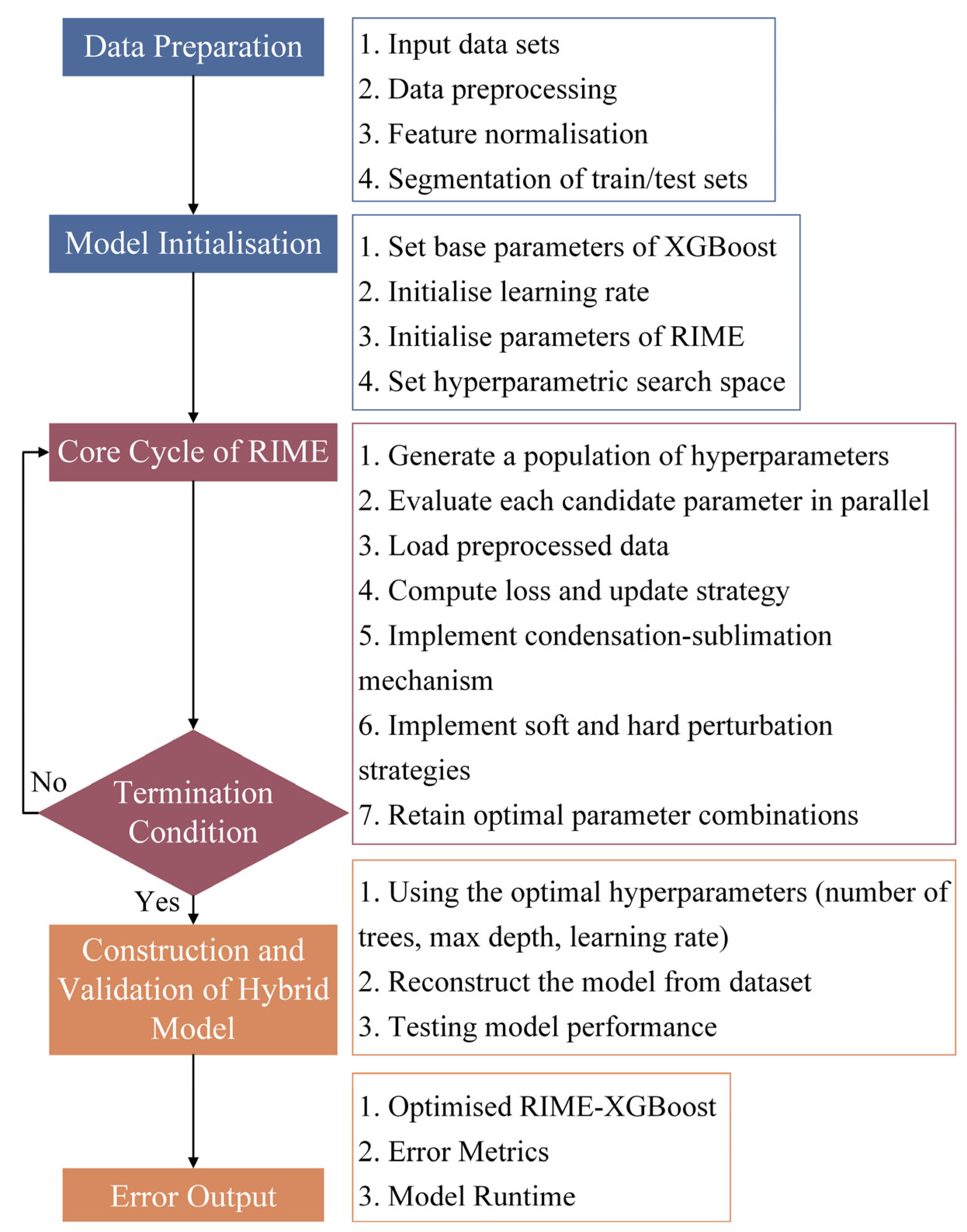
3.3. RIME-Optimized XGBoost Hybrid Model

XGBoost was chosen as the base model, with its three hyperparameters (number of trees, tree depth, learning rate) optimized simultaneously using RIME. XGBoost adapts to different scales of input samples, thereby enhancing its learning and generalization capabilities. A hybrid model with high learning and generalization abilities is established, as illustrated in Figure 3.

XGBoost does not have a built-in, fully automated hyperparameter optimization tool. Hyperparameter settings usually depend on experience or are assisted by strategies like early stopping, cross-validation, and grid search.

However, these methods have flaws or limitations. For example, grid search and cross-validation consume a lot of computing resources and time, while setting empirical parameters requires a lot of prior knowledge and understanding of the model and data. Moreover, hyperparameters influence each other, and traditional optimization methods may not handle this well. They may lead to suboptimal tuning results.

In this study, we use RIME with MSE as the loss function to simultaneously optimize the number of trees, tree depth, and learning rate of XGBoost. The process includes the following:

(1) Mapping XGBoost’s three core hyperparameters to RIME’s optimization goals, forming its search space, where each parameter combination is a potential solution.

(2) Setting the value range and step size for hyperparameters.

(3) Using MSE as the fitness function to evaluate each parameter combination.

(4) Setting the population size and randomly generating individuals within the parameter range.

(5) Iteratively optimizing based on RIME’s calculation mechanism.

(6) Returning the optimal hyperparameter combination to XGBoost upon convergence or reaching the maximum iteration.

(7) Training XGBoost and generating predictions.

4. Comparative Study and Error Quantification

4.1. Comparative Methods

The comparison models are hybrid models from recently published journal papers. They include Slime Mould Algorithm-optimized Random Forest (RF) [39], Snake Optimizer-optimized BiGRU [40], and Equilibrium Optimizer-optimized Support Vector Regression (SVR) [41]. Detailed information about them is shown in

Table 3. Detailed information about comparative items (hybrid models).

Name (Abbreviation)	Advantages of Hybrid Modeling	Hyperparameter
SMA-RF	Reduce computational cost and improve generalization ability	Number of decision trees: [10, 300] Minimum number of leaf nodes: [10, 300]
SO-BiGRU	Enhance prediction accuracy and generalization ability and accelerate model convergence	Initial learning rate: [1 × 10−4, 1 × 10−1] Number of neurons in GRU layer: [3, 50] L2 regularization parameter: [1 × 10−6, 1 × 10−2]
EO-SVR	Escape local optima and better balance model complexity and fitting error	Penalty factor: [1, 2000] Radial basis function kernel parameter: [1 × 10−2, 10]

.

These three comparison models cover a variety of machine learning methods and optimization algorithms. The setup ensures model diversity. RF is a classic ensemble learning method suitable for modeling high-dimensional data. It has strong robustness and anti-overfitting capabilities [42]. BiGRU belongs to deep learning and is particularly suitable for processing sequential data. It can capture long-term dependencies in the data [43]. SVR is suitable for small-sample modeling and establishing nonlinear mappings. It uses kernel functions to map from low-dimensional data to high-dimensional spaces, solving complex problems [44].

Therefore, by comparing different combinations of optimization algorithms and models, this study comprehensively evaluates the performance of RIME-XGBoost. It verifies its effectiveness across different scenarios and data scales. Moreover, the comparison models are all from published journal papers, enhancing persuasiveness and credibility.

4.2. Error Measurement Metrics

This section summarizes key metrics for quantifying prediction accuracy and computational efficiency, along with their comparative advantages and limitations.

Root Mean Square Error (RMSE) measures the magnitude of prediction errors by averaging squared residuals and taking their root. It shares the same unit as the target variable but amplifies outlier effects due to squaring. A higher RMSE indicates larger deviations between predictions ${\widehat{y}}_i$ and true values $y_i$.

MSE computes the average squared error, emphasizing large discrepancies. While sensitive to outliers, it avoids the unit conversion required by RMSE. Mean Absolute Error (MAE) quantifies average absolute deviations, offering robustness to outliers. Unlike RMSE/MSE, MAE is scale-dependent and interpretable.

Mean Bias Error (MBE) indicates systematic bias by averaging prediction errors. A positive/negative MBE reflects overestimation/underestimation. R-squared captures the proportion of variance in $y_i$ explained by the model. Ranging from 0 to 1, it assesses overall fit quality and is dimensionless, enabling cross-model comparisons.

Moreover, Runtime represents the total time for training/testing cycles. It compares models’ balance of accuracy and resource demands.

$$\mathrm{RMSE}=\sqrt{{\displaystyle \frac{1}{n}}\sum _{i=1}^n{(y_i-{\widehat{y}}_i)}^2}$$

(9)

$$\mathrm{MSE}={\displaystyle \frac{1}{n}}\sum _{i=1}^n{(y_i-{\widehat{y}}_i)}^2$$

(10)

$$\mathrm{MAE}={\displaystyle \frac{1}{n}}\sum _{i=1}^n|y_i-{\widehat{y}}_i|$$

(11)

$$\mathrm{MBE}={\displaystyle \frac{1}{n}}{\displaystyle \sum _{i=1}^n}({\widehat{y}}_i-y_i)$$

(12)

$$R^2=1-{\displaystyle \frac{{\displaystyle \sum _{i=1}^n}{(y_i-{\widehat{y}}_i)}^2}{{\displaystyle \sum _{i=1}^n}{(y_i-\overline{y})}^2}}$$

(13)

5. Rotor Temperature Modeling and Prediction

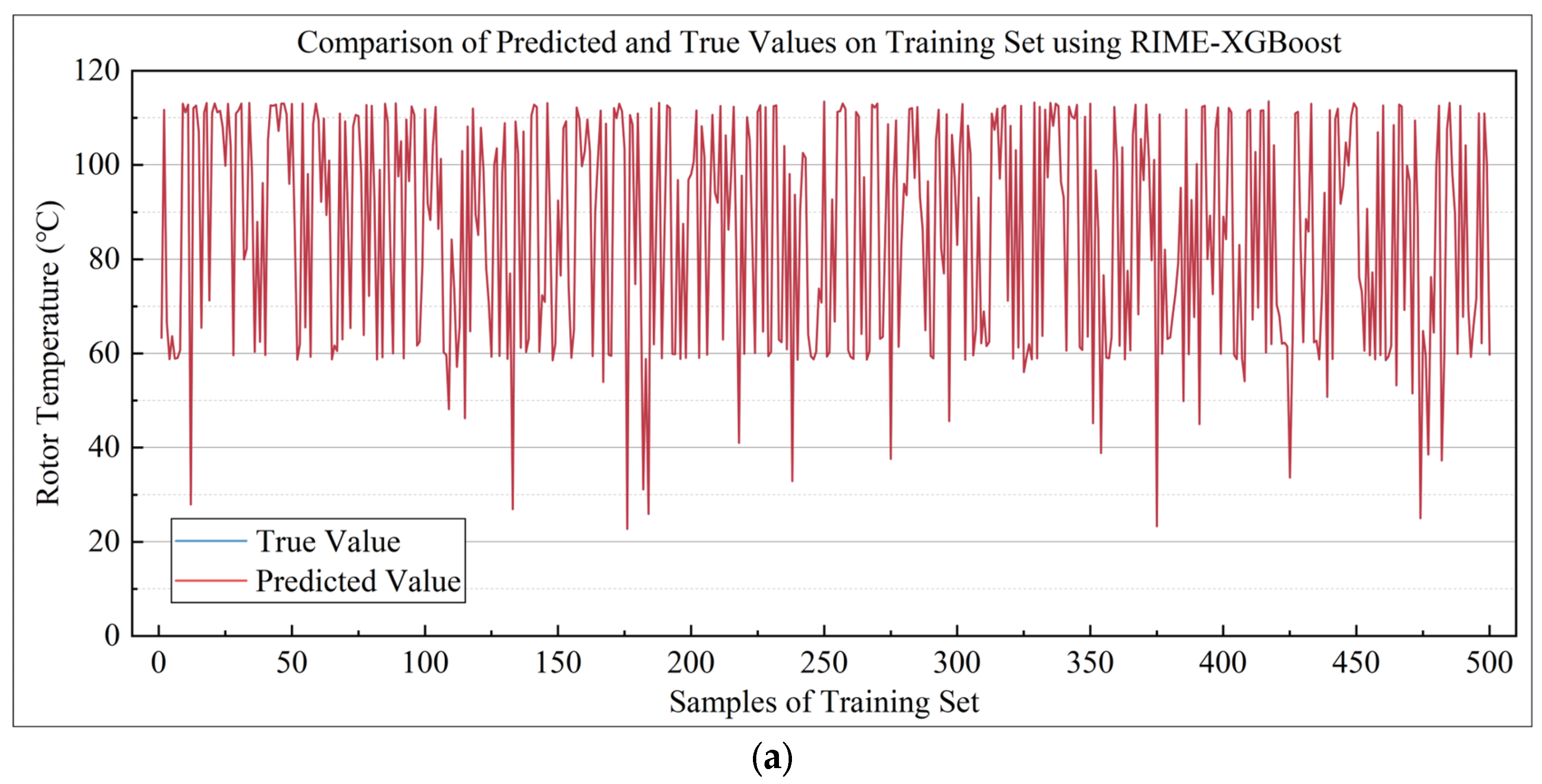
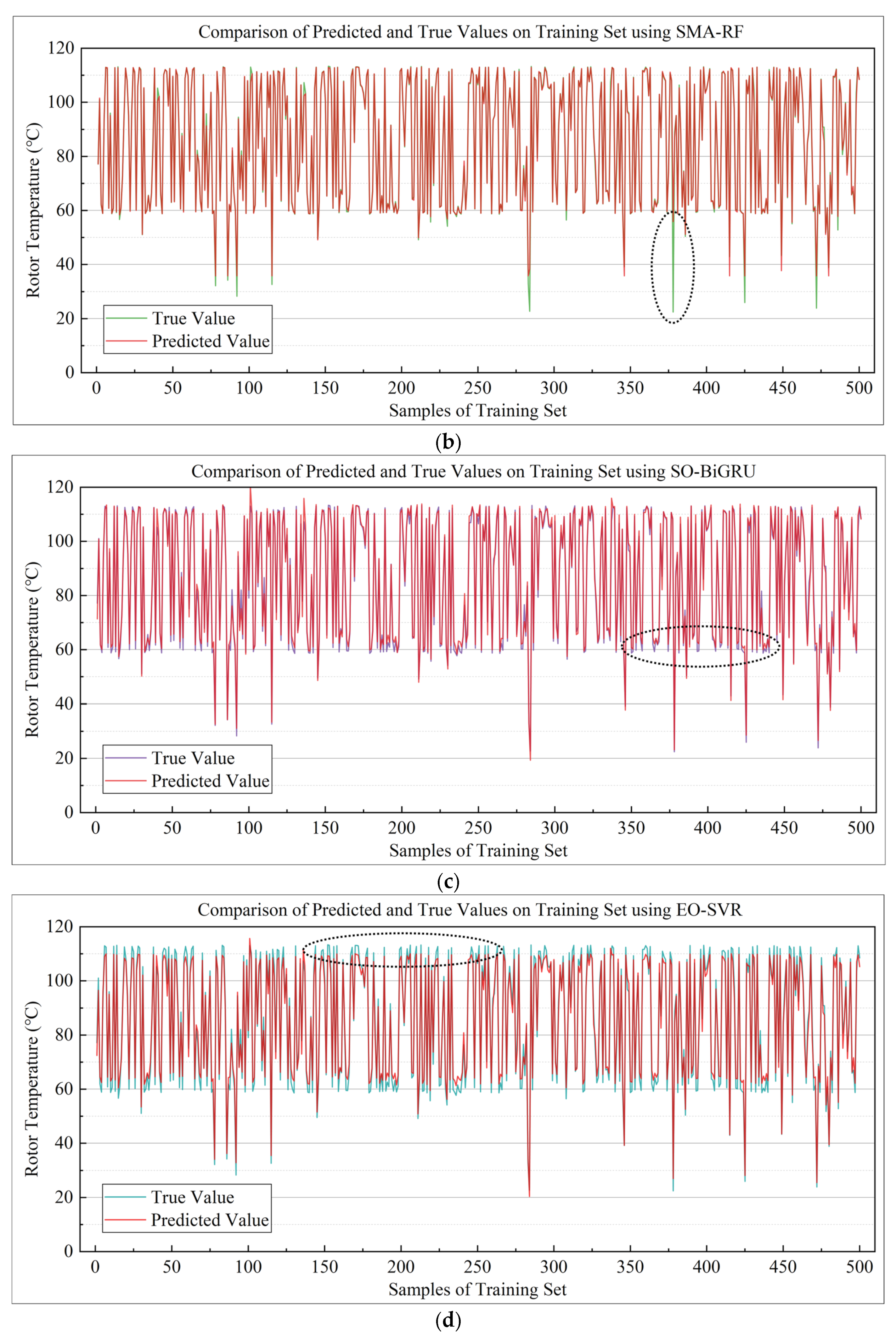
5.1. Rotor Temperature Prediction Experiment Under Medium-Sized Samples

Rotor temperature is a critical indicator of PMSMs’ operating conditions. The accurate prediction of rotor temperature helps to optimize motor performance, extend equipment lifespan, and prevent failures. This section conducts experiments using the sample from Group A. The input features are multiple easily monitored parameters during PMSM operation (current, voltage, speed, etc.), and the target variable is the rotor temperature. The rotor temperature ranges from a minimum of 21.93 °C to a maximum of 113.61 °C, covering a wide spectrum from low to high temperatures.

Testing model performance across a wide temperature range allows for a more comprehensive evaluation of its adaptability. For instance, it assesses whether the model performs well in low-, medium-, and high-temperature intervals. In practical applications, motor rotor temperatures are likely to fluctuate significantly. Therefore, medium-scale samples can simulate some typical real-world scenarios.

To avoid randomness in the test results, RIME-XGBoost and the three comparison models are trained and predicted sequentially for 20 consecutive times. The accuracy, prediction bias, generalization ability, and computational efficiency of the hybrid methods are evaluated using RMSE, MSE, MAE, MBE, R-squared (R²), and Runtime (the duration of one round of training and testing).

Subsequently, the population and iterations of each hybrid model are set as shown in

Table 4. Algorithm parameters of hybrid models.

	RIME-XGBoost	SMA-RF	SO-BiGRU	EO-SVR
Population	20	20	10	30
Iteration	20	30	5	50

. The hardware configuration of the computer used in the experiment is as follows: Intel Core i7-11800H processor (Intel, Santa Clara, CA, USA), Samsung DDR4 3200 MHz 16 GB RAM (Samsung, Suwon, Republic of Korea), and NVIDIA GeForce RTX 3060 6 GB GPU (Nvidia, Santa Clara, CA, USA). The training and testing results are presented in

Table 5. Results of rotor temperature prediction experiment with medium-sized samples.

Model	Stage	Error	Average	Median	Standard Deviation
RIME-XGBoost	Train	RMSE	0.0440	0.0442	0.0016
		MSE	0.0019	0.0020	0.0001
		MAE	0.0318	0.0321	0.0013
		MBE	2.84 × 10−5	9.42 × 10−6	5.53 × 10−5
		R-squared	0.9999	0.9999	2.17 × 10−7
	Test	RMSE	1.1555	1.0298	0.4079
		MSE	1.5016	1.0605	1.1670
		MAE	0.4864	0.4782	0.0410
		MBE	−0.0227	−0.0185	0.0478
		R-squared	0.9972	0.9981	0.0021
	Total	Runtime	52.9506	51.3548	4.9756
SMA-RF	Train	RMSE	1.7814	1.7963	0.2987
		MSE	3.2625	3.2269	1.0684
		MAE	0.7109	0.7136	0.0706
		MBE	0.0456	0.0463	0.0364
		R-squared	0.9940	0.9942	0.0020
	Test	RMSE	2.2036	2.0456	0.3157
		MSE	4.9554	4.1855	1.4704
		MAE	0.9034	0.8913	0.0705
		MBE	0.0689	0.0787	0.0936
		R-squared	0.9909	0.9923	0.0027
	Total	Runtime	28.3762	28.5778	1.8633
SO-BiGRU	Train	RMSE	1.9903	2.0787	0.4596
		MSE	4.1726	4.3210	2.0399
		MAE	1.4642	1.4852	0.3535
		MBE	−0.0946	−0.0334	0.4265
		R-squared	0.9923	0.9920	0.0037
	Test	RMSE	4.4236	3.4068	3.1639
		MSE	29.5780	11.6067	47.3067
		MAE	1.6525	1.6125	0.3797
		MBE	−0.0933	−0.0437	0.4356
		R-squared	0.9457	0.9785	0.0867
	Total	Runtime	302.5257	297.2967	17.3790
EO-SVR	Train	RMSE	2.9917	3.0152	0.1205
		MSE	8.9648	9.0911	0.7025
		MAE	2.7001	2.7252	0.1351
		MBE	0.0658	0.0417	0.1639
		R-squared	0.9897	0.9898	0.0008
	Test	RMSE	3.5104	3.3311	0.5031
		MSE	12.5763	11.0971	3.7286
		MAE	2.8003	2.8138	0.0863
		MBE	0.0854	0.1177	0.1648
		R-squared	0.9835	0.9878	0.0074
	Total	Runtime	25.1217	24.3481	2.4326

.

First, the performance of each model is analyzed. RIME-XGBoost performs exceptionally well on the training set, with an RMSE of 0.044, MSE of 0.0019, MAE of 0.032, and R-squared close to 1 (0.9999). It demonstrates an extremely high degree of fit to the training data. Additionally, the MBE is close to 0, indicating minimal prediction bias. On the test set, R-squared remains high (0.9972), while RMSE and MSE show slight increases. Although the variability of the predictions increases, the generalization ability remains strong. The average Runtime is 52.95 s, significantly lower than that of SO-BiGRU, indicating moderate computational complexity.

SMA-RF shows lower errors on the training set, with an RMSE of 1.7814. The R-squared value suggests a high degree of fit to the training data. The MBE is 0.0456, indicating a small positive prediction bias. On the test set, RMSE and MSE increase slightly, while R-squared remains at 0.9909. Its average computation time is 28.37 s, demonstrating high computational efficiency. However, SMA-RF’s overall performance in both training and testing is inferior to RIME-XGBoost.

EO-SVR exhibits similar prediction performance and computational efficiency to SMA-RF. However, its MBE is larger, indicating a higher positive prediction bias. The test set results are relatively stable, but their prediction accuracy is weaker than that of SMA-RF.

SO-BiGRU is the worst-performing hybrid model overall. Its average modeling time is significantly longer than that of RIME-XGBoost (approximately 5.7 times). While the training set R-squared is high, the predictions show a negative bias. During testing, all of the error metrics increase, indicating poor generalization ability. The standard deviation results suggest instability in the prediction process.

Furthermore, as shown in Figure 4, although all hybrid models achieve low errors on the training set, the three methods, excluding RIME-XGBoost, have limitations. For example, SMA-RF struggles to provide accurate predictions at low temperatures and fails to fit sudden temperature drops. SO-BiGRU cannot predict fluctuating data in the low-temperature region. EO-SVR is unable to accurately learn fluctuating data in both high- and low-temperature regions, resulting in minor errors between the predicted and actual values.

A half-violin plot using the MAE of the test set is shown in Figure 5. The horizontal axis represents the models, and the vertical axis represents the MAE. It is visually evident that RIME-XGBoost is the most stable method, while SO-BiGRU has the largest error distribution. In terms of average values, RIME-XGBoost is the lowest. SMA-RF is a moderately performing model. However, in one out of the twenty tests, an anomaly occurred, which increased the overall prediction error and variability. The MAE distribution of EO-SVR shows a bimodal pattern, indicating two concentrated forms of prediction errors. This suggests that the model’s learning ability varies depending on the randomly selected training data. EO-SVR’s prediction performance is significantly influenced by the data, demonstrating its weak robustness.

Therefore, it is clear that RIME-XGBoost performs best in terms of prediction accuracy, generalization ability, and stability. In contrast, SO-BiGRU, despite its high R-squared value on the training set, exhibits unstable performance on the test set and has extremely high computational complexity. EO-SVR and SMA-RF show relatively good overall performance, but their prediction accuracy is lower than that of RIME-XGBoost.

The robustness of RIME-XGBoost under varying temperature conditions highlights its potential for real-world industrial applications. Unlike SMA-RF and EO-SVR, which exhibit significant bias in specific temperature ranges (e.g., EO-SVR’s underprediction in high-temperature regions), RIME-XGBoost’s minimal bias across the entire temperature spectrum suggests its adaptability to diverse operational scenarios.

It is critical for EV applications to be diverse where sudden temperature fluctuations (e.g., during rapid acceleration or braking) are common. Furthermore, RIME-XGBoost’s computational efficiency aligns with real-time monitoring requirements in high-speed motor systems. It is a viable candidate for embedded systems with limited computational resources.

Under medium-scale sample conditions, RIME-XGBoost demonstrates excellent prediction performance. However, whether it can maintain high accuracy in rotor temperature prediction under small-sample conditions remains to be further verified. Therefore, the next section will test and discuss the small-sample modeling performance of RIME-XGBoost.

5.2. Rotor Temperature Modeling and Prediction Under Small Samples

Experiments under small-sample conditions not only verify the robustness of RIME-XGBoost but also highlight how limited data directly impact the accuracy of model decisions. Moreover, in practical applications, factors such as cost, space, and motor design constraints often make data collection and storage challenging. Thus, small-sample experiments simulate these real-world scenarios. This section conducts experiments based on the Group B dataset.

The hybrid models still undergo 20 consecutive rounds of training and prediction to avoid randomness in the test results. The error evaluation metrics and the computer hardware used for the experiments remain unchanged. The population and iterations of each hybrid model are slightly adjusted, as shown in

Table 6. Algorithm parameters of each hybrid model.

	RIME-XGBoost	SMA-RF	SO-BiGRU	EO-SVR
Population	20	50	10	30
Iteration	20	50	10	50

. The training and testing results are presented in

Table 7. Results of rotor temperature prediction experiment under small-sample conditions.

Model	Stage	Error	Average	Median	Standard Deviation
RIME-XGBoost	Train	RMSE	0.0068	0.0068	0.0004
		MSE	0.0000	0.0000	0.0000
		MAE	0.0050	0.0050	0.0003
		MBE	1.23 × 10−6	−1.04 × 10−6	7.08 × 10−6
		R-squared	0.9999	0.9999	1.09 × 10−6
	Test	RMSE	0.6010	0.5960	0.0741
		MSE	0.3667	0.3553	0.0913
		MAE	0.4020	0.4015	0.0429
		MBE	0.0149	0.0180	0.0748
		R-squared	0.9491	0.9455	0.0107
	Total	Runtime	47.4799	47.3804	1.5684
SMA-RF	Train	RMSE	0.6295	0.5911	0.1417
		MSE	0.4163	0.3494	0.2044
		MAE	0.3941	0.3716	0.0773
		MBE	0.0322	0.0217	0.0382
		R-squared	0.9427	0.9504	0.0273
	Test	RMSE	0.8937	0.8773	0.2180
		MSE	0.8463	0.7697	0.4081
		MAE	0.6043	0.5951	0.1177
		MBE	0.0508	0.0241	0.1763
		R-squared	0.8865	0.8941	0.0486
	Total	Runtime	47.0174	46.6430	6.1770
SO-BiGRU	Train	RMSE	0.7036	0.6963	0.0818
		MSE	0.5018	0.4849	0.1143
		MAE	0.5591	0.5705	0.0754
		MBE	0.0014	0.0008	0.0030
		R-squared	0.9302	0.9294	0.0165
	Test	RMSE	0.8069	0.7890	0.0914
		MSE	0.6594	0.6225	0.1459
		MAE	0.6409	0.6314	0.0734
		MBE	0.0087	0.0150	0.1145
		R-squared	0.9119	0.9146	0.0214
	Total	Runtime	176.0875	176.1744	1.4659
EO-SVR	Train	RMSE	0.5598	0.5539	0.0282
		MSE	0.3142	0.3068	0.0318
		MAE	0.4820	0.4756	0.0286
		MBE	−0.0647	−0.0602	0.0339
		R-squared	0.9588	0.9582	0.0066
	Test	RMSE	0.6777	0.6722	0.0639
		MSE	0.4634	0.4519	0.0908
		MAE	0.5435	0.5429	0.0377
		MBE	−0.0631	−0.0637	0.0992
		R-squared	0.9458	0.9495	0.0109
	Total	Runtime	6.2627	6.2731	0.6984

.

RIME-XGBoost demonstrates extremely high accuracy and stability on the training set, but its performance on the test set slightly declines, suggesting potential overfitting. However, its metrics on the test set are still superior to those of the comparison models. SMA-RF shows relatively consistent performance on both the training and test sets. Its overall error is higher, indicating weaker capability in capturing features from small-sample data. SO-BiGRU has significantly longer computation times than other models, with prediction accuracy at a moderate level. EO-SVR performs well, especially on the training set, but its performance on the test set slightly declines. Despite its short modeling time, its overall performance is suboptimal.

By combining the standard deviations of the error metrics, the stability of each model across the 20 consecutive prediction experiments is compared. Although RIME-XGBoost shows some fluctuations on the test set, its high R-squared value and low standard deviation indicate good stability. EO-SVR also demonstrates good stability. However, SMA-RF and SO-BiGRU have higher standard deviations, indicating greater variability in their predictions.

A two-dimensional scatter plot of all hybrid models on the training and test sets is shown in Figure 6. The horizontal axis represents the true values, and the vertical axis represents the predicted values. The diagonal line in the plot represents perfect prediction, where predicted values equal true values. RIME-XGBoost performs well overall, with only a few predicted values slightly lower than the true values near 92 °C. SMA-RF exhibits a clear bias in the temperature range of 78, 86°C, where predicted values are generally higher than the true values. In higher temperature ranges, SMA-RF performs better.

In Figure 6, SO-BiGRU’s predictions do not show a clear unidirectional bias. However, overall observations reveal that some predicted values are higher than the true values, while others are lower. There is a lack of consistency between the predicted and true values, resulting in larger overall errors. Finally, EO-SVR tends to underpredict in high-temperature regions and overpredict in low-temperature regions, indicating significant prediction biases across different temperature ranges. In contrast, RIME-XGBoost demonstrates more stable and reliable predictions across all temperature ranges.

Figure 7 presents a dual-Y-axis boxplot using the R-squared and RMSE of the test set. It visually illustrates the prediction errors of each model. The R-squared distribution of SMA-RF is too wide, ranging approximately from 0.78 to 0.96. Its reliability is low, as its predictions are unstable in practical applications. RIME-XGBoost has the highest mean and median R-squared values. Its box length is the shortest, indicating excellent prediction consistency. The RMSE shows similar results: the mean RMSE of RIME-XGBoost is around 0.6, while that of SMA-RF is around 0.9. EO-SVR demonstrates good prediction stability, but its mean and median RMSE are approximately 0.7. SO-BiGRU is a moderate hybrid model, with relatively small error values but significant variability.

In the small-sample experiments, RIME-XGBoost and EO-SVR are the two standout models. The former performs exceptionally well on the training set and demonstrates strong generalization on the test set. The latter has the highest computational efficiency but slightly lower overall accuracy. SMA-RF and SO-BiGRU fail to deliver satisfactory test results.

The stark contrast between the model’s near-perfect training performance (R² = 0.9999) and its lower test set accuracy (R² = 0.9491) signals a classic case of overfitting. This gap likely stems from excessive model complexity or inadequate regularization, where the algorithm memorizes training data patterns rather than learning generalizable trends.

To bridge this performance divide in RIME-XGBoost, targeted adjustments can enhance generalization without sacrificing predictive power. While RIME already optimizes core hyperparameters like tree quantity, depth, and learning rate, introducing additional regularization constraints may curb overfitting. For instance, setting a minimum loss reduction threshold prevents trees from splitting on insignificant or noisy patterns. Increasing weight penalty terms discourages the model from relying excessively on individual features.

Furthermore, not all features contribute equally to generalization. By systematically retaining high-impact predictors while discarding redundant or irrelevant variables, the pruning process reduces the risk of spurious correlations. When implemented in concert, these strategies contribute to simplifying the model architecture and improving generalization.

5.3. Performance Comparison Between RIME-XGBoost and Baseline XGBoost

As discussed in Section 5.1 and Section 5.2, the comprehensive predictive performance of RIME-XGBoost surpasses that of several comparable hybrid models. Section 5.3 evaluates the performance of RIME-XGBoost against baseline XGBoost models using empirical parameters. The goal is to investigate whether the hyperparameters optimized by RIME significantly outperform heuristic settings and to determine if RIME effectively addresses the limitations of XGBoost in hyperparameter selection.

Two sets of commonly used empirical parameters were designed for the baseline XGBoost models, as shown in

Table 8. Hyperparameter settings for two typical baseline XGBoost models.

Model	Number of Trees	Tree Depth	Learning Rate
XGBoost-Alpha	50	5	0.05
XGBoost-Beta	300	15	0.005

. The first parameter set is tailored for simpler prediction tasks. It employs fewer trees to avoid overfitting, shallower tree depths to prevent excessive model complexity, and a moderate learning rate. The configuration is termed XGBoost-Alpha.

The second parameter set is designed for more complex regression tasks. It uses a larger number of trees and deeper tree depths to enhance model precision, coupled with a smaller learning rate to ensure stable convergence. This configuration is referred to as XGBoost-Beta.

First, baseline models were evaluated using Group A, with 20 prediction experiments conducted separately. The data partitioning strategy and computational hardware remained consistent across all the experiments.

Table 9. Performance evaluation based on error metrics of RIME-XGBoost and baseline models on Group A (medium-scale).

Model	Stage	Error	Average	Median	Standard Deviation
RIME-XGBoost	Train	RMSE	0.0440	0.0442	0.0016
		MSE	0.0019	0.0020	0.0001
		MAE	0.0318	0.0321	0.0013
		MBE	2.84 × 10−5	9.42 × 10−6	5.53 × 10−5
		R-squared	0.9999	0.9999	2.17 × 10−7
	Test	RMSE	1.1555	1.0298	0.4079
		MSE	1.5016	1.0605	1.1670
		MAE	0.4864	0.4782	0.0410
		MBE	−0.0227	−0.0185	0.0478
		R-squared	0.9972	0.9981	0.0021
	Total	Runtime	52.9506	51.3548	4.9756
XGBoost-Alpha	Train	RMSE	2.3286	2.3308	0.0623
		MSE	5.4261	5.4325	0.2887
		MAE	1.9056	1.9028	0.0614
		MBE	1.3008	1.3051	0.0903
		R-squared	0.9900	0.9901	0.0005
	Test	RMSE	2.7128	2.6569	0.2273
		MSE	7.4084	7.0594	1.2525
		MAE	2.0269	2.0355	0.0432
		MBE	1.2814	1.3351	0.1039
		R-squared	0.9863	0.9870	0.0023
	Total	Runtime	0.5361	0.3879	0.6124
XGBoost-Beta	Train	RMSE	6.7034	6.6945	0.1096
		MSE	44.9465	44.8168	1.4738
		MAE	5.5201	5.5063	0.1260
		MBE	3.9315	3.9234	0.1789
		R-squared	0.9171	0.9172	0.0032
	Test	RMSE	6.9004	6.8938	0.0993
		MSE	47.6243	47.5249	1.3725
		MAE	5.6420	5.6478	0.0485
		MBE	3.9833	3.9951	0.0793
		R-squared	0.9122	0.9124	0.0024
	Total	Runtime	0.5342	0.3799	0.6368

presents the average and median values and standard deviations of the error metrics.

RIME-XGBoost demonstrates a clear superiority over the baseline models in the experimental evaluations. On the test set, its RMSE is notably lower (only 40% of XGBoost-Alpha’s and 16% of XGBoost-Beta’s), which highlights its generalization ability. RIME-XGBoost achieves an R² score of 0.9972 on the test set, nearly matching the training set’s 0.9999. The consistency underscores its resistance to overfitting, which is a challenge partially addressed but not fully resolved by the baselines. They exhibit higher error rates and variability.

The results also show the pitfalls of empirical parameter tuning. XGBoost-Alpha, with its limited tree count and shallow depths, underfits the data due to insufficient complexity, as seen in its persistent positive bias (MBE) on the test set. It is a sign of poor accuracy for high-value predictions.

Meanwhile, XGBoost-Beta’s deeper trees and larger ensemble size lead to instability, resulting in elevated errors. These outcomes reveal that conventional parameters struggle to balance predictive performance and precision for XGBoost. In contrast, RIME’s optimized hyperparameters provide a harmonious synergy that increases model robustness and reduces the reliance on trial-and-error tuning.

Subsequently, 20 prediction experiments were conducted using the Group B dataset the for baseline models. The average values and standard deviations of all the error metrics are summarized in

Table 10. Performance evaluation based on error metrics of RIME-XGBoost and baseline models on Group B (small-scale).

Model	Stage	Error	Average	Median	Standard Deviation
RIME-XGBoost	Train	RMSE	0.0068	0.0068	0.0004
		MSE	0.0000	0.0000	0.0000
		MAE	0.0050	0.0050	0.0003
		MBE	1.23 × 10−6	−1.04 × 10−6	7.08 × 10−6
		R-squared	0.9999	0.9999	1.09 × 10−6
	Test	RMSE	0.6010	0.5960	0.0741
		MSE	0.3667	0.3553	0.0913
		MAE	0.4020	0.4015	0.0429
		MBE	0.0149	0.0180	0.0748
		R-squared	0.9491	0.9455	0.0107
	Total	Runtime	47.4799	47.3804	1.5684
XGBoost-Alpha	Train	RMSE	0.4443	0.4456	0.0251
		MSE	0.1980	0.1986	0.0223
		MAE	0.3575	0.3636	0.0229
		MBE	0.2488	0.2526	0.0185
		R-squared	0.9748	0.9753	0.0032
	Test	RMSE	0.8240	0.7992	0.1017
		MSE	0.6888	0.6387	0.1770
		MAE	0.6192	0.6087	0.0553
		MBE	0.2720	0.2871	0.0990
		R-squared	0.8977	0.9047	0.0177
	Total	Runtime	0.3359	0.3276	0.0292
XGBoost-Beta	Train	RMSE	1.0984	1.1127	0.0642
		MSE	1.2104	1.2381	0.1367
		MAE	0.9745	0.9871	0.0634
		MBE	0.7655	0.7684	0.0599
		R-squared	0.8373	0.8377	0.0184
	Test	RMSE	1.2480	1.2134	0.1456
		MSE	1.5777	1.4723	0.3938
		MAE	1.0448	1.0288	0.0958
		MBE	0.7317	0.7591	0.1560
		R-squared	0.7830	0.7918	0.0429
	Total	Runtime	0.4117	0.2716	0.6223

.

In small-sample scenarios, RIME-XGBoost outperforms the two baseline models in terms of predicting rotor temperature. XGBoost-Alpha has a higher test set RMSE than RIME-XGBoost but is better than XGBoost-Beta. The MBE still shows a systematic positive bias.

XGBoost-Beta has multiple test set errors significantly higher than other models, suggesting severe overfitting in small samples. Its average R² is only 0.7830. The model fails to learn data patterns effectively.

However, RIME-XGBoost has potential overfitting risks. The significant difference between the test set and training set R² indicates that the model may fail to balance complexity due to insufficient data in small samples. The model structure is too complex. Moreover, its training set RMSE is close to 0, and the MSE is almost 0, implying possible overfitting on the training set.

By comparing baseline models using different empirical parameters, we can see RIME-XGBoost’s pros and cons. It still has lower errors in small samples, which proves the effectiveness of RIME in hyperparameter optimization. Optimizing the number of trees, tree depth, and learning rate enhances learning ability and reduces overfitting.

The limitations of RIME-XGBoost are the need to design additional regularization strategies or optimize regularization parameters to further balance prediction accuracy, generalization, and computational efficiency. For example, regularization parameters and early-stopping have to be introduced to expand RIME-XGBoost. In addition, the operation logic of RIME-XGBoost can be changed. Using GPU parallel computing can shorten its Runtime.

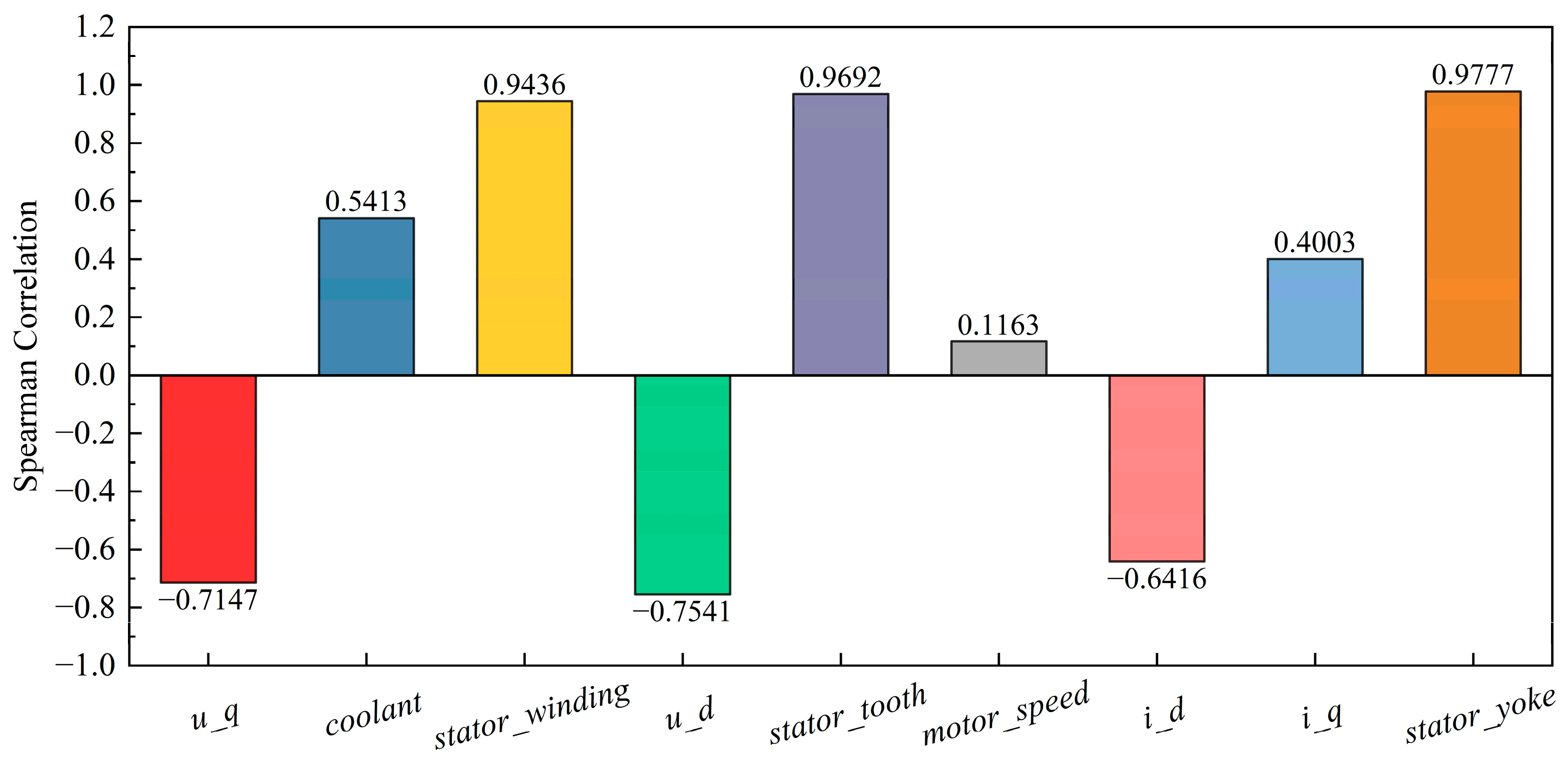
5.4. Spearman Correlation Analysis of Rotor Temperature Dependencies in PMSMs

In motor systems, the relationship between rotor temperature and electrical/mechanical parameters often exhibits nonlinear characteristics. Compared to Pearson’s linear assumption, Spearman’s nonparametric nature, which relies on the ranks of variables, can effectively analyze monotonic nonlinear associations. Moreover, Spearman is less sensitive to outliers and the distribution shape of data, while motor sensor data frequently contain noise or pulse interference. Therefore, Spearman’s correlation coefficient is more appropriate than Pearson or other correlation coefficients. First, the analysis was conducted using Group A, and the results are shown in Figure 8.

stator_yoke (0.9777), stator_tooth (0.9692), and stator_winding (0.9436) exhibit an extremely strong positive correlation with rotor temperature (pm). This phenomenon stems from the internal thermal conduction paths within the motor. The current in the stator winding generates Joule heat, which is conducted through the tooth to the yoke. Ultimately, heat transfers to the permanent magnets via heat conduction across the air gap and limited convection. These three parameters are highly suitable as indirect indicators for monitoring rotor temperature.

u_d (−0.7541) and u_q (−0.7147) show significant negative correlations. In the vector control of a PMSM, the d-axis voltage is used for field-weakening control to extend the motor’s high-speed operating range and may indirectly affect iron losses. The q-axis voltage regulates the torque current. These negative correlations might reflect a mechanism where the controller actively increases voltage under high-temperature conditions to compensate for reduced counter electromotive force. It suppresses heat accumulation.

coolant and i_q are moderately correlated variables. When coolant temperature rises, reduced heat dissipation capability accelerates heat accumulation, consistent with thermal equilibrium principles. However, their correlation coefficients are lower than those of stator components. This suggests a potential thermal response lag in the cooling system. The q-axis current is proportional to motor torque. Its relatively lower correlation may arise from current-limiting control strategies implemented by the controller during high-temperature operation.

motor_speed shows no significant correlation with rotor temperature, which contradicts intuitive expectations. This could be due to the compensation effect of closed-loop control strategies or the absence of high-speed, heavy-load operational data in the experimental dataset.

Subsequently, Spearman’s correlation analysis was performed using Group B, and the results are shown in Figure 9.

The results of the two Spearman analyses exhibit discrepancies. The differences are primarily reflected in three aspects: (1) reversal of correlation coefficient signs for voltage components (u_d, u_q), (2) fluctuating strengths of correlations for stator temperature parameters, and (3) reduced correlation for coolant temperature.

These discrepancies likely arise due to sensitivity to small sample sizes. In other words, a single outlier can significantly alter the rank of variables, and the presence of certain samples may disrupt overall monotonicity. Furthermore, the reduced experimental sample size may lead to insufficient coverage of the operational conditions space.

For the design of PMSMs, the discrepancies between the two analyses provide new insights. The rotor temperature in PMSMs exhibits coupled characteristics, and the dominant heat transfer mechanisms may vary across different operating points. For scenarios such as low/high speed or heavy/light load, temperature prediction models can be constructed using combinations of physical parameters tailored to specific conditions.

5.5. Enhancement of Motor Optimization and Adaptability of RIME-XGBoost

This study intentionally focused on developing a robust baseline model using commonly available operational parameters (speed, torque, d-q currents/voltages) that are standard across most PMSM implementations. It offers a practical value for EV manufacturers without requiring additional sensor infrastructure.

The RIME-XGBoost framework offers two inherent adaptability advantages:

(1) The optimization approach enables efficient fine-tuning with small new datasets when applied to different motor designs.

(2) The hybrid model can naturally incorporate additional input parameters (e.g., coolant flow rate, ambient temperature) through simple feature engineering.

RIME-XGBoost establishes a data-driven predictive model for PMSM rotor temperature by leveraging easily monitored operational variables (e.g., d-q-axis currents/voltages, torque, speed). It circumvents the need for direct rotor temperature sensors. Thus, it reduces hardware costs while enhancing the intelligence of thermal management systems. The integration of RIME-XGBoost with adaptive thermal management policies can provide a foundation for motor optimization, for instance, enabling the exploration of smaller cooling systems or higher magnetic saturation thresholds.

The adaptability of RIME-XGBoost to new PMSMs arises from the integration of RIME’s optimization capabilities and XGBoost’s robust ensemble learning framework. The hybrid approach achieves transfer learning through hyperparameter adaptation.

RIME employs a gradient-free optimization mechanism that facilitates rapid convergence to optimal configurations. By dynamically re-optimizing key parameters (number of trees, tree depth, and learning rate), the model can strike a balance between retaining prior knowledge and adapting to specific domains.

The experimental results on medium- and small-sample datasets demonstrate the adaptability of RIME-XGBoost. This hybrid approach ensures transfer learning across different conditions while maintaining efficiency and accuracy.

5.6. In-Depth Discussion on Model Performance

In both experiments, RIME-XGBoost, SMA-RF, SO-BiGRU, and EO-SVR optimized their hyperparameters using different optimization algorithms. RIME-XGBoost accurately learned the relationship between input features and rotor temperature in both medium-scale and small-scale samples, making it the best-performing model overall. A deeper discussion from the perspectives of the base model and optimization algorithm reveals the reasons for its excellent prediction performance.

RIME-XGBoost uses RIME to optimize the number of trees, tree depth, and learning rate of XGBoost. XGBoost, an ensemble learning method, excels at establishing complex nonlinear relationships, often resulting in high training set fitting. In addition, XGBoost incorporates regularization terms, effectively preventing overfitting.

RIME efficiently finds the optimal hyperparameter combination through a combination of global search and local optimization, further enhancing the model’s learning and generalization capabilities. The ensemble learning mechanism, hyperparameter tuning, and built-in regularization collectively contribute to RIME-XGBoost’s prediction performance.

In comparison, SMA-RF performs suboptimally but has high computational efficiency. RF, based on Bagging ensemble learning, has strong anti-overfitting capabilities and can be trained in parallel. It is suitable for medium- to large-scale data. However, as the number of decision trees and the minimum leaf size increase, computational complexity rises significantly. SMA optimizes two hyperparameters, which enhances SMA-RF’s overall capabilities.

SO-BiGRU’s weakness lies in the instability of its prediction results in each round, along with the highest computational complexity. Although BiGRU can learn long-term dependencies in sequential data, recurrent neural networks are highly sensitive to hyperparameter choices. An insufficient hyperparameter search can lead to poor prediction performance. Furthermore, the complex structure of BiGRU and excessive population and iteration choices in the optimization algorithm result in exceptionally long Runtimes per round. This tradeoff between prediction performance and computational efficiency limits its applicability.

Finally, EO-SVR shows moderate performance but limited prediction accuracy. SVR can learn nonlinear relationships in data and is robust to outliers. The main limitation of EO-SVR is its relatively low prediction accuracy. In other words, while EO efficiently searches the hyperparameter space, the SVR hyperparameter space may contain multiple local optima, preventing the optimization result from being globally optimal. Hyperparameters tuned by EO enhance SVR’s performance. However, SVR’s sensitivity to hyperparameters still restricts further performance improvements. Increasing the population and iterations of the optimization algorithm might address this issue.

Therefore, selecting RIME-XGBoost for building a rotor temperature prediction model is the optimal solution. The ensemble learning mechanism, collaborative optimization of multiple hyperparameters, and regularization settings collectively enhance its prediction accuracy and generalization ability.

6. Conclusions

Accurate rotor temperature prediction in PMSMs is critical for improving operational reliability and prolonging service life. This study proposes RIME-XGBoost, which synergizes metaheuristic optimization with ensemble learning to address the challenges of modeling rotor temperature under varying data conditions. By integrating dynamic parameters (e.g., motor speed, torque, d-q-axis current voltage) through a multi-source feature fusion strategy, the model achieves robust performance across medium-scale datasets with pronounced thermal fluctuations (Group A) and small-sample high-temperature regimes (Group B).

The hybrid framework of RIME-XGBoost uniquely balances precision and computational efficiency. The key findings include the following:

(1) RIME-XGBoost surpasses comparable hybrid models by delivering precise predictions on medium-sized datasets. Although its performance diminishes slightly on smaller datasets, it remains effective, whereas other models falter.

(2) RIME-XGBoost employs a hybrid strategy to optimize critical parameters, balancing precision, stability, and computational efficiency. It also identifies intricate relationships between input data and rotor temperature.

(3) SMA-RF, while swift due to its parallel architecture, struggles with limited data. SO-BiGRU suffers from slow training and sensitivity to hyperparameters. EO-SVR, though stable, is less accurate than RIME-XGBoost due to hyperparameter dependencies and optimization limitations.

(4) In industrial applications, the developed model reduces dependence on physical sensors and maintenance expenses. It minimizes manual tuning requirements and establishes a foundation for proactive thermal management and extending motor lifespan.

Future work will prioritize three directions: (1) Testing under diverse environmental conditions (e.g., extreme temperatures, variable loads) and motor architectures. (2) Developing adaptive feature selection and hyperparameter tuning pipelines to minimize manual intervention. (3) Deploying lightweight variants on embedded systems for real-time thermal monitoring.

References

1. Littlejohn, C.; Proost, S. What Role for Electric Vehicles in the Decarbonization of the Car Transport Sector in Europe? Econ. Transp. 2022, 32, 100283. [Google Scholar] [CrossRef]
2. Kubik, A.; Turoń, K.; Folęga, P.; Chen, F. CO2 Emissions—Evidence from Internal Combustion and Electric Engine Vehicles from Car-Sharing Systems. Energies 2023, 16, 2185. [Google Scholar] [CrossRef]
3. Teng, Z.; Tan, C.; Liu, P.; Han, M. Analysis on Carbon Emission Reduction Intensity of Fuel Cell Vehicles from a Life-Cycle Perspective. Front. Energy 2024, 18, 16–27. [Google Scholar] [CrossRef]
4. Ercan, T.; Onat, N.C.; Keya, N.; Tatari, O.; Eluru, N.; Kucukvar, M. Autonomous Electric Vehicles Can Reduce Carbon Emissions and Air Pollution in Cities. Transp. Res. Part D Transp. Environ. 2022, 112, 103472. [Google Scholar] [CrossRef]
5. Akrami, M.; Jamshidpour, E.; Pierfederici, S.; Frick, V. Flatness-Based Trajectory Planning/Replanning for a Permanent Magnet Synchronous Machine Control. In Proceedings of the 2023 IEEE Transportation Electrification Conference & Expo (ITEC), Detroit, MI, USA, 21 June 2023; pp. 1–5. [Google Scholar]
6. Song, Y.; Lu, J.; Hu, Y.; Wu, X.; Wang, G. Fast Calibration with Raw Data Verification for Current Measurement of Dual-PMSM Drives. IEEE Trans. Ind. Electron. 2024, 71, 6875–6885. [Google Scholar] [CrossRef]
7. Rigatos, G.; Abbaszadeh, M.; Wira, P.; Siano, P. A Nonlinear Optimal Control Approach for Voltage Source Inverter-Fed Three-Phase PMSMs. In Proceedings of the IECON 2021—47th Annual Conference of the IEEE Industrial Electronics Society, Toronto, ON, Canada, 13 October 2021; pp. 1–6. [Google Scholar]
8. Pandey, A.; Madduri, B.; Perng, C.-Y.; Srinivasan, C.; Dhar, S. Multiphase Flow and Heat Transfer in an Electric Motor. In Proceedings of the Volume 8: Fluids Engineering; Heat Transfer and Thermal Engineering. American Society of Mechanical Engineers: Columbus, OH, USA, 2022; p. V008T10A034. [Google Scholar]
9. Liu, L.; Ding, S.; Liu, C.; Zhang, D.; Wang, Q. Electromagnetic Performance Analysis and Thermal Research of an Outer-rotor I-shaped Flux-switching Permanent-magnet Motor with Considering Driving Cycles. IET Electr. Power Appl. 2019, 13, 2052–2057. [Google Scholar] [CrossRef]
10. Meiwei, Z.; Weili, L.; Haoyue, T. Demagnetization Fault Diagnosis of the Permanent Magnet Motor for Electric Vehicles Based on Temperature Characteristic Quantity. IEEE Trans. Transp. Electrif. 2023, 9, 759–770. [Google Scholar] [CrossRef]
11. Lima, R.P.G.; Mauricio Villanueva, J.M.; Gomes, H.P.; Flores, T.K.S. Development of a Soft Sensor for Flow Estimation in Water Supply Systems Using Artificial Neural Networks. Sensors 2022, 22, 3084. [Google Scholar] [CrossRef]
12. Ahmed, U.; Ali, F.; Jennions, I. Acoustic Monitoring of an Aircraft Auxiliary Power Unit. ISA Trans. 2023, 137, 670–691. [Google Scholar] [CrossRef]
13. Gudur, B.R.; Poddar, G.; Muni, B.P. Parameter Sensitivity on the Performance of Sensor-Based Rotor Flux Oriented Vector Controlled Induction Machine Drive. Sādhanā 2023, 48, 169. [Google Scholar] [CrossRef]
14. Hu, J.; Sun, Z.; Xin, Y.; Jia, M. Real-Time Prediction of Rotor Temperature with PMSMs for Electric Vehicles. Int. J. Therm. Sci. 2025, 208, 109516. [Google Scholar] [CrossRef]
15. Kang, M.; Shi, T.; Guo, L.; Gu, X.; Xia, C. Thermal Analysis of the Cooling System with the Circulation between Rotor Holes of Enclosed PMSMs Based on Modified Models. Appl. Therm. Eng. 2022, 206, 118054. [Google Scholar] [CrossRef]
16. Song, B.-K.; Chin, J.-W.; Kim, D.-M.; Hwang, K.-Y.; Lim, M.-S. Temperature Estimation Using Lumped-Parameter Thermal Network with Piecewise Stator-Housing Modules for Fault-Tolerant Brake Systems in Highly Automated Driving Vehicles. IEEE Trans. Intell. Transp. Syst. 2021, 22, 5819–5832. [Google Scholar] [CrossRef]
17. Pereira, M.; Araújo, R.E. Model-Free Finite-Set Predictive Current Control with Optimal Cycle Time for a Switched Reluctance Motor. IEEE Trans. Ind. Electron. 2023, 70, 8355–8364. [Google Scholar] [CrossRef]
18. Kumar, J.A.; Swaroopan, N.M.J.; Shanker, N.R. Prediction of Rotor Slot Size Variations in Induction Motor Using Polynomial Chirplet Transform and Regression Algorithms. Arab. J. Sci. Eng. 2023, 48, 6099–6109. [Google Scholar] [CrossRef]
19. Ye, C.; Deng, C.; Yang, J.; Dai, Y.; Yu, D.; Zhang, J. Study on a Novel Hybrid Thermal Network of Homopolar Inductor Machine. IEEE Trans. Transp. Electrif. 2023, 9, 549–560. [Google Scholar] [CrossRef]
20. Zhou, H.; Wang, X.; Zhao, W.; Liu, J.; Xing, Z.; Peng, Y. Rapid Prediction of Magnetic and Temperature Field Based on Hybrid Subdomain Method and Finite-Difference Method for the Interior Permanent Magnet Synchronous Motor. IEEE Trans. Transp. Electrif. 2024, 10, 6634–6651. [Google Scholar] [CrossRef]
21. Bouziane, M.; Bouziane, A.; Naima, K.; Alkhafaji, M.A.; Afenyiveh, S.D.M.; Menni, Y. Enhancing Temperature and Torque Prediction in Permanent Magnet Synchronous Motors Using Deep Learning Neural Networks and BiLSTM RNNs. AIP Adv. 2024, 14, 105136. [Google Scholar] [CrossRef]
22. Cuiping, L.; Pujia, C.; Shukang, C.; Feng, C. Research on Motor Iron Losses and Temperature Field Calculation for Mini Electric Vehicle. In Proceedings of the 2014 17th International Conference on Electrical Machines and Systems (ICEMS), Hangzhou, China, 22 October 2014; pp. 2380–2383. [Google Scholar]
23. Ayvaz, S.; Alpay, K. Predictive Maintenance System for Production Lines in Manufacturing: A Machine Learning Approach Using IoT Data in Real-Time. Expert Syst. Appl. 2021, 173, 114598. [Google Scholar] [CrossRef]
24. Kirchgassner, W.; Wallscheid, O.; Bocker, J. Data-Driven Permanent Magnet Temperature Estimation in Synchronous Motors with Supervised Machine Learning: A Benchmark. IEEE Trans. Energy Convers. 2021, 36, 2059–2067. [Google Scholar] [CrossRef]
25. Zhang, X.; Hu, Y.; Zhang, J.; Xu, H.; Sun, J.; Li, S. Domain-Adversarial Adaptation Regression Model for IPMSM Permanent Magnet Temperature Estimation. IEEE Trans. Transp. Electrif. 2025, 11, 4383–4394. [Google Scholar] [CrossRef]
26. Jing, H.; Chen, Z.; Wang, X.; Wang, X.; Ge, L.; Fang, G.; Xiao, D. Gradient Boosting Decision Tree for Rotor Temperature Estimation in Permanent Magnet Synchronous Motors. IEEE Trans. Power Electron. 2023, 38, 10617–10622. [Google Scholar] [CrossRef]
27. Jing, H.; Xiao, D.; Wang, X.; Chen, Z.; Fang, G.; Guo, X. Temperature Estimation of Permanent Magnet Synchronous Motors Using Support Vector Regression. In Proceedings of the 2022 25th International Conference on Electrical Machines and Systems (ICEMS), Chiang Mai, Thailand, 29 November 2022; pp. 1–6. [Google Scholar]
28. Zhang, Z.; Zhang, Y.; Wen, Y.; Ren, Y. Data-Driven XGBoost Model for Maximum Stress Prediction of Additive Manufactured Lattice Structures. Complex Intell. Syst. 2023, 9, 5881–5892. [Google Scholar] [CrossRef]
29. Xu, H.-W.; Qin, W.; Sun, Y.-N. An Improved XGBoost Prediction Model for Multi-Batch Wafer Yield in Semiconductor Manufacturing. IFAC-PapersOnLine 2022, 55, 2162–2166. [Google Scholar] [CrossRef]
30. Jin, R.; Huang, H.; Li, L.; Zuo, H.; Gan, L.; Ge, S.S.; Liu, Z. Artificial Intelligence Enabled Energy-Saving Drive Unit with Speed and Displacement Variable Pumps for Electro-Hydraulic Systems. IEEE Trans. Autom. Sci. Eng. 2024, 21, 3193–3204. [Google Scholar] [CrossRef]
31. Li, D.; Zhu, D.; Tao, T.; Qu, J. Power Generation Prediction for Photovoltaic System of Hose-Drawn Traveler Based on Machine Learning Models. Processes 2023, 12, 39. [Google Scholar] [CrossRef]
32. Pan, Z.; Fang, S. Torque Performance Improvement of Permanent Magnet Arc Motor Based on Two-Step Strategy. IEEE Trans. Ind. Inf. 2021, 17, 7523–7534. [Google Scholar] [CrossRef]
33. Lin, B.; Wang, D.; Ni, Y.; Song, K.; Li, Y.; Sun, G. Temperature Prediction of Permanent Magnet Synchronous Motor Based on Data-Driven Approach. In Proceedings of the 2024 36th Chinese Control and Decision Conference (CCDC), Xi’an, China, 25 May 2024; pp. 3270–3275. [Google Scholar]
34. Shimizu, Y.; Morimoto, S.; Sanada, M.; Inoue, Y. Using Machine Learning to Reduce Design Time for Permanent Magnet Volume Minimization in IPMSMs for Automotive Applications. IEEJ J. Ind. Appl. 2021, 10, 554–563. [Google Scholar] [CrossRef]
35. Shimizu, Y. Efficiency Optimization Design That Considers Control of Interior Permanent Magnet Synchronous Motors Based on Machine Learning for Automotive Application. IEEE Access 2023, 11, 41–49. [Google Scholar] [CrossRef]
36. Kirchgassner, W.; Wallscheid, O.; Bocker, J. Estimating Electric Motor Temperatures with Deep Residual Machine Learning. IEEE Trans. Power Electron. 2021, 36, 7480–7488. [Google Scholar] [CrossRef]
37. Chen, T.; Guestrin, C. XGBoost: A Scalable Tree Boosting System. In Proceedings of the 22nd ACM SIGKDD International Conference on Knowledge Discovery and Data Mining, San Francisco CA, USA, 13 August 2016; pp. 785–794. [Google Scholar]
38. Su, H.; Zhao, D.; Heidari, A.A.; Liu, L.; Zhang, X.; Mafarja, M.; Chen, H. RIME: A Physics-Based Optimization. Neurocomputing 2023, 532, 183–214. [Google Scholar] [CrossRef]
39. Khajavi, H.; Rastgoo, A. Predicting the Carbon Dioxide Emission Caused by Road Transport Using a Random Forest (RF) Model Combined by Meta-Heuristic Algorithms. Sustain. Cities Soc. 2023, 93, 104503. [Google Scholar] [CrossRef]
40. Lei, W.; Gu, X.; Zhou, L. A Deep Learning Model Based on the Introduction of Attention Mechanism Is Used to Predict Lithium-Ion Battery SOC. J. Electrochem. Soc. 2024, 171, 070508. [Google Scholar] [CrossRef]
41. Houssein, E.H.; Dirar, M.; Abualigah, L.; Mohamed, W.M. An Efficient Equilibrium Optimizer with Support Vector Regression for Stock Market Prediction. Neural Comput. Appl. 2022, 34, 3165–3200. [Google Scholar] [CrossRef]
42. Breiman, L. Random Forests. Mach. Learn. 2001, 45, 5–32. [Google Scholar] [CrossRef]
43. Schuster, M.; Paliwal, K.K. Bidirectional Recurrent Neural Networks. IEEE Trans. Signal Process. 1997, 45, 2673–2681. [Google Scholar] [CrossRef]
44. Smola, A.J.; Schölkopf, B. A Tutorial on Support Vector Regression. Stat. Comput. 2004, 14, 199–222. [Google Scholar] [CrossRef]
Figure 1. A test setup featuring a representative PMSM with comparable specifications [36].
Applsci 15 03688 g001
Figure 2. Flowchart of data processing and utilization.
Applsci 15 03688 g002
Figure 3. Hybrid modeling process of RIME-XGBoost.
Applsci 15 03688 g003
Figure 4. (a) Prediction on the training set using RIME-XGBoost. (b) Prediction on the training set using SMA-RF. (c) Prediction on the training set using SO-BiGRU. (d) Prediction on the training set using EO-SVR.
Applsci 15 03688 g004aApplsci 15 03688 g004b
Figure 5. Half-violin plot of MAE for these models on the medium-scale test set.
Applsci 15 03688 g005
Figure 6. Scatter plot comparing true and predicted values across training and test sets.
Applsci 15 03688 g006aApplsci 15 03688 g006b
Figure 7. Boxplot with dual-Y-axes: R-squared and RMSE of test set across models.
Applsci 15 03688 g007
Figure 8. Spearman correlation between features and rotor temperature in Group A.
Applsci 15 03688 g008
Figure 9. Spearman correlation between features and rotor temperature in Group B.
Applsci 15 03688 g009