Adaptive Beamforming Damage Imaging of Lamb Wave Based on CNN

Abstract

Among damage imaging methods based on Lamb waves, the Minimum Variance Distortionless Response (MVDR) method adaptively calculates channel weights to suppress interference signals, improving imaging resolution and the signal-to-noise ratio (SNR). However, the MVDR method involves matrix inversion, which introduces a high computational burden to the implementation process and makes real-time damage detection challenging. We propose constructing a Convolutional-Neural-Network (CNN)-based network architecture based on the Delay-and-Sum (DAS) beamforming method. This architecture replaces the MVDR’s adaptive weight calculation by establishing a nonlinear mapping from multi-channel data to weighting factors, enabling efficient high-resolution Lamb wave damage imaging with an enhanced SNR. To verify the effectiveness and imaging performance of the CNN-based method, damage in an aluminum plate is imaged using both simulation and experimental methods. The imaging results are compared and analyzed against those of the DAS and MVDR methods. The results show that the proposed CNN-based adaptive Lamb wave beamforming method, which combines the advantages of a high resolution and signal-to-noise ratio, as well as rapid imaging, can provide reference and support for real-time Lamb-wave-based Structural Health Monitoring (SHM).

1. Introduction

Lamb waves, as an effective tool for damage detection and assessment of plate structures, have the advantages of low attenuation, long propagation distance, and sensitivity to structural surface and internal damage [1,2]. In order to visualize the damage in structures, many scholars have proposed and developed a large number of Lamb wave imaging methods, such as beamforming [3,4], phased array imaging [5], and neural network [6] methods. These methods help to identify and assess potential problems in structures more clearly, thereby improving the efficiency and accuracy of detection and monitoring.

DAS and MVDR beamforming techniques have been widely used in Lamb wave damage imaging methods. Yu et al. [7] successfully achieved the imaging identification of crack damage in aluminum plates using the DAS method based on a phased array of one-dimensional piezoelectric wafer active sensors. Veidt et al. [8] achieved the detection and localization of structural damage using the DAS beamforming method with signals extracted from a network consisting of four sensors only. Khodaei et al. [9] proposed an improved DAS method, which achieved imaging of impact damage in composite plates by adding windows to the received signals. Tian et al. [10] acquired Lamb wave signals using a completely non-contact method and used an improved DAS algorithm to achieve damage imaging of aluminum plates. Although DAS is a simple and effective damage imaging method, one of its main shortcomings is the poor suppression of undesired interference signals. To improve the performance of Lamb wave damage imaging, Michaels et al. [11] introduced the MVDR method to the nondestructive testing of distributed arrays. Subsequently, Hall et al. [12] demonstrated through damage imaging experiments on aluminum plates that the MVDR method can significantly improve the image quality compared to DAS. Engholm et al. [13] found that the MVDR method improves the suppression of interfering Lamb modes using uniform rectangular arrays and exhibits higher resolution and better sidelobe and mode suppression. Hua et al. [14] used the MVDR algorithm, which incorporated local signal correlation coefficients as damage features, thereby improving the performance of Lamb wave damage imaging by providing more reliable damage indicators. Xu et al. [15] proposed a weighted sparse decomposition coefficients-based MVDR method and validated it in quasi-isotropic composite laminates. Peng et al. [16] proposed an adaptive diagonal loading MVDR method, which improves the imaging quality of the conventional MVDR method. The above studies have facilitated the application of MVDR methods in the field of Lamb wave SHM. However, the MVDR method requires computing adaptive weights by inverting the covariance matrix, which not only encounters the problem of matrix ill-conditioning but also has high computational complexity, leading to a significant increase in imaging time and making real-time SHM challenging.

With the development of machine learning techniques, deep learning networks have been used for damage detection based on ultrasound guided waves [17,18,19]. Su et al. [20] collected the scattering signals of Lamb waves interacting with various types of defects experimentally, obtained the amplitude-frequency characteristics of these signals by using fast Fourier transform, and then utilized these characteristics as inputs to a deep neural network model. This approach established a mapping relationship between the amplitude-frequency characteristics of the scattering signals and the damage locations, thereby achieving accurate defect localization. Song et al. [21] proposed a sub-wavelength defect super resolution visualization method by using the U-Net network to extract the defect edge information of ultrasound images and achieved subwavelength imaging of defects. Zhang et al. [22] proposed a semi-supervised deep convolutional neural network probabilistic imaging algorithm by using a CNN to automatically extract DI in the guided wave signals and output the probabilistic image of the damage, achieving the damage imaging detection of aluminum and composite panels, which demonstrated good material generalization. Wang et al. [23] proposed a sparse guided wave imaging algorithm based on compressed perception and a deep learning model to solve the problem that the imaging quality is constrained by the number of transducers and achieved the quantitative assessment of corrosion damage of aluminum plates by establishing the mapping relationship between the guided wave signals and corrosion imaging of aluminum plates. Sheng et al. [24] introduced a deep-learning-based adaptive beamforming technique, which achieved high-resolution imaging of damage in plate structures by dynamically adjusting the apodization weights for pixel input data from the transducers using a Fully Connected Neural Network (FCNN). The above research shows that deep neural networks can be well-applied to structural damage detection by establishing a correct and generalized mapping from input to output. Although MVDR methods can improve damage imaging resolution and reduce imaging artifacts, they are, however, limited by the low imaging efficiency caused by the inverse computation of channel weights on the covariance matrix. We propose leveraging deep learning for data mapping and introducing a CNN to directly map delay-corrected Lamb wave scattering signals to the weights of each channel, thereby improving imaging performance and efficiency. This approach provides technical support for the real-time online SHM of Lamb waves.

The remainder of this paper is organized as follows: Section 2 describes the conventional DAS and MVDR imaging methods; Section 3 details the design and training strategy of the CNN neural network architecture proposed in this paper; Section 4 discusses the simulation and experimental results and quantitatively compares and analyzes the performance of the different imaging methods; and the conclusions are presented in Section 5.

2. Beamforming Imaging Method

2.1. DAS Method

In the DAS beamforming imaging algorithm, the imaging region is usually divided into grids, and the pixel value of each grid point P(x, y) corresponds to an imaging index. For different imaging points, combined with the array layout, the imaging index can be obtained by applying appropriate delay to the received signals, and the delay of each array element can be calculated by the following equation:

$$t_n\left(x,y\right)=t_0+{\displaystyle \frac{\sqrt{{\left(x-x_0\right)}^2+{\left(y-y_0\right)}^2}+\sqrt{{\left(x-x_n\right)}^2+{\left(y-y_n\right)}^2}}{c_g}}$$

(1)

where $t_0$ is the time point corresponding to the maximum amplitude of the excitation signal, $x_0$ and $y_0$ are the coordinates of the target imaging point, $x_n$ and $y_n$ are the coordinates of the excitation array elements and are the coordinates of the receiving array elements, n = 1, 2, …, N, N is the number of elements in the array, and $c_g$ is the group velocity of the Lamb wave. For different imaging points in the imaging region, the signal amplitude after delay is as follows:

$$z_n(x,y)=s_n\left(t_n\right(x,y\left)\right)$$

(2)

where $s_n\left(t_n\right)$ denotes the damage scattering signal received by the nth array element of the array. To optimize the resolution and contrast of the imaging results, a preset apodization weight vector $\mathbf{w}(x,y)$, such as the Hanning window, is introduced to weight and sum the signal vectors $\mathit{z}(x,y)$ of the received channels. Apodization—the process of applying spatially varying weights to sensor channels—adjusts the amplitude distribution of signals during beamforming. This technique enhances imaging performance by suppressing sidelobe interference and sharpening the main lobe, thereby improving noise reduction and spatial resolution. The image $I_{\mathrm{DAS}}(x,y)$ generated by the DAS method can be obtained as follows:

$$I_{\mathrm{DAS}}(x,y)={\mathbf{w}}^{\mathrm{T}}(x,y)\cdot \mathbf{z}(x,y)$$

(3)

2.2. MVDR Method

Since the weighting vectors of the DAS method are fixed and preset without considering the characteristics of the received data, the performance improvement of imaging is limited. In contrast, the weighting vector is computed with the MVDR method, whose goal is to ensure that the pixel value of the target point in the imaging region is 1 and to minimize the output power. Therefore, the weight vector can be obtained by solving the following constrained optimization problem [25]:

$$\underset{\mathit{w}}{\min }{\mathbf{w}}^{\mathrm{T}}{\mathit{R}}_{xy}\mathbf{w}\hspace{1em}\hspace{1em}s.t.{\mathbf{w}}^{\mathrm{T}}\mathbf{e}=1$$

(4)

where ${\mathit{R}}_{xy}$ denotes the sampling covariance matrix and e is the unit orientation vector. Solving Equation (4) yields the following:

$${\mathbf{w}}_{\mathrm{MV}}={\displaystyle \frac{{\mathit{R}}_{xy}^{-1}\mathbf{e}}{{\mathbf{e}}^{\mathrm{T}}{\mathit{R}}_{xy}^{-1}\mathbf{e}}}$$

(5)

Since the sampled data have been previously corrected for delays based on the target pixel point locations, there is $\mathbf{e}=1$. In order to avoid possible instability during matrix inversion, regularization is usually performed using the diagonal loading method, i.e.,

$${\mathit{R}}_{xy}^{-1}=({\mathit{R}}_{xy}+\epsilon {\lambda }_1\mathbf{I}{)}^{-1}$$

(6)

where ${\lambda }_1$ is the maximum eigenvalue of ${\mathit{R}}_{xy}$, and $\epsilon$ is the regularization factor. Accordingly, the pixel value at position P in the image output from the MVDR method is as follows:

$$I_{\mathrm{MVDR}}(x,y)={\mathbf{w}}_{\mathrm{MV}}^{\mathrm{T}}\mathbf{z}$$

(7)

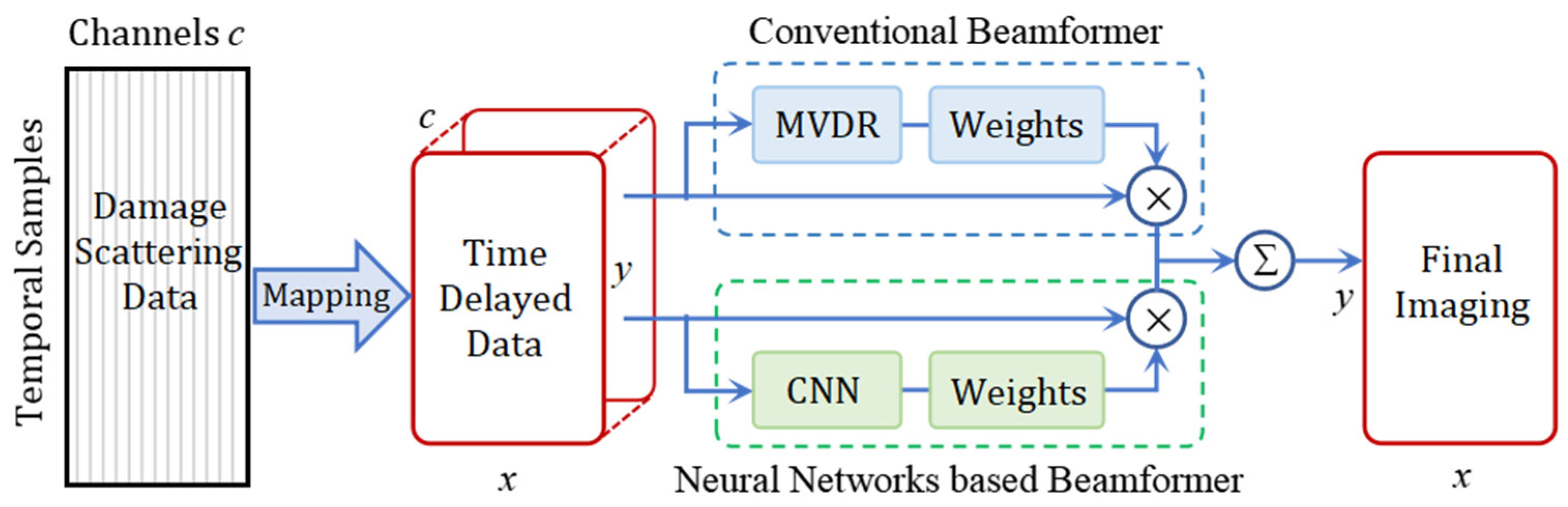
3. Adaptive Beamforming Model Based on CNN

3.1. Network Model Architecture

Figure 1 gives a schematic diagram from damage scattering data to final imaging. First, the scattering data are delayed according to the positions of different imaging points, and a 3D matrix is generated by time–space mapping, where the third dimension is the number of channels. Then, the adaptive beamforming method is utilized to calculate the channel weights corresponding to each pixel point. Inspired by the adaptive MVDR method, the designed neural network adaptively computes the weight factors by inputting delayed channel data. Thus, the costly MVDR method for weight calculation is replaced by a more computationally efficient neural network, and this design aims to achieve the adaptive adjustment of weights for different imaging points in the imaging region through network prediction. For different imaging points, the pixel value is obtained by computing the inner product of the delay-corrected array channel data $\mathit{z}$ and the weights $f\left(\mathit{z}\right)$ predicted by the neural network:

$$I_{\mathrm{CNN}}=f(\mathit{z}{)}^{\mathrm{T}}\cdot \mathit{z}$$

(8)

The CNN network architecture is shown in Figure 2. The architecture of the CNN beamformer consists of an input layer, four hidden convolutional layers, and an output layer. The dimension of the input layer is (Nx, Ny, Nc), where Nx, Ny, and Nc are the x, y coordinates and the number of transducers (channels) in the imaging region, respectively. In order to ensure the stability of the training, the input channel data are subsequently subjected to L2 regularization, which penalizes excessively large weight values to prevent overfitting [26]. Specifically, a regularization term $\lambda \sum w_i^2$ is incorporated into the loss function, where $\lambda$ controls the strength of the penalty and $w_i$ denotes the network weights. This approach enhances model robustness by discouraging over-reliance on individual channel features while maintaining the integrity of the training process. In this case, 8-array received signals are used in both simulations and experiments, and the real and imaginary parts of the received resolved signals are considered. The number of points in the imaging region is 201 by 101. Therefore, the value of (Nx, Ny, Nc) in the text is (201, 101, 16). The input layer is followed by four hidden layers, each containing a 2D convolutional layer, an activation layer, and a batch regularization layer. Each convolutional layer has a 7 × 7 filter kernel size and a convolutional output, and the output feature map has the same height and width as the input. The activation function used in the hidden layers is an anti-rectifier unit, which prevents negative input values from being mapped to zero. This design mitigates the risk of ’dead neurons’—a scenario where neurons cease updating their weights during training due to prolonged zero outputs—by ensuring continuous gradient flow and maintaining neuronal activity even for negative inputs, thereby enhancing the network’s learning stability and generalization capabilities. Batch regularization is used in each convolutional layer to further improve stability during training. In the hidden layer, the number of filters is increased from 32 to 64 in two incremental steps at a rate of 2, and finally back to 16 channel counts. The output layer of the network provides individual channel adaptive apodization weights corresponding to each pixel in the input layer, so the output dimension matches the input dimension, which is (Nx, Ny, Nc). To ensure that the sum of the apodization weights for all channels at each pixel in the output layer equals unity, a Softmax activation function is employed [27]. This choice aligns with the unity constraint ($\sum w_i$ = 1) imposed in the MVDR algorithm—a critical requirement for beamforming. Unlike ReLU, which produces unbounded outputs, Softmax inherently generates probabilistic weights by pushing higher values toward 1 and lower values toward 0. This property not only enforces the MVDR optimization objective but also suppresses contributions from noise-corrupted channels during beamforming.

The proposed CNN architecture is a novel design tailored for Lamb wave beamforming, integrating time–space mapping, anti-rectifier activation, and Softmax-based weight normalization to address the challenges of adaptive imaging. In this framework, the input to the CNN beamformer is the Time of Flight Corrected (ToFC) data, while the output of the CNN beamformer is the corresponding apodization weights of each channel for different imaging points in the imaging region. These apodization weights are then multiplied with the ToFC data from the input layer and summed along the channel axes to produce the final beamforming image. For clarity, the pseudocode of the proposed CNN-based adaptive beamforming workflow is outlined below:

Algorithm: CNN-based adaptive beamforming workflow.

Input: Multi-channel Lamb wave signals $\mathit{z}$.

Output: Damage image $I_{CNN}$.

(1)

Preprocess input signals:

–

Apply Time-of-Flight Correction (ToFC) to align scattered signals.

–

Extract real and imaginary parts (channel dimension: 16 for 8 receivers).

(2)

Feed ToFC data into the CNN:

–

Input dimensions: 201 $\times$ 101 $\times$ 16.

–

Process through four convolutional layers (7 × 7 kernels, anti-rectifier activation).

–

Apply batch normalization and L2 regularization.

(3)

Predict apodization weights ${\mathbf{w}}_{CNN}$:

–

Softmax activation ensures $\sum {\mathbf{w}}_{CNN}=\mathbf{1}$.

(4)

Compute pixel values:

–

$I_{CNN}={{\mathbf{w}}_{CNN}}^{\mathbf{T}}\cdot \mathit{z}$.

(5)

Generate the final image by aggregating pixel values across the grid.

3.2. Network Training Strategies

The network is trained using the Adam optimizer [24], an adaptive learning rate algorithm that combines the advantages of momentum-based gradient descent and RMSProp. Adam dynamically adjusts learning rates for each parameter by estimating the first and second moments of gradients, enabling efficient convergence even with sparse or noisy data. The initial learning rate is set to 1 × 10⁻⁴, which balances the training stability and convergence speed for our task. The training process optimizes the loss function by processing each random batch, which contains all the pixels from a single image. The stochastic training strategy ensures that the sequence of data provided to the network in each training round is randomized. The total training loss of the network includes the image loss, which is designed to promote similarity between the target image and the image generated by the network. Since the proposed CNN model predicts continuous weighting factors rather than discrete classes, regression metrics are used instead of classification metrics like confusion matrices. The traditional MSE loss function is computationally efficient and straightforward to optimize, measuring the error magnitude by calculating the squared difference between predicted and true values. This approach not only reduces noise sensitivity but also provides a robust reflection of the model’s performance, aligning well with the regression nature of the task. Therefore, the network training image loss function used is MSE, denoted as L_MSE.

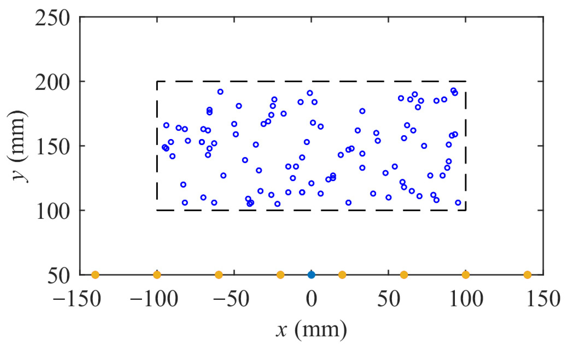
3.3. Acquisition of Training Data Sets

In order to provide enough training and validation data for the CNN, this paper utilizes the theory of unimodal Lamb wave propagation to simulate and calculate the generation of relevant datasets required for CNN training. Assuming that there exists a point damage P(x, y) in the damage detection region, the distance from the excitation point to the damage point and the distance from the damage point to the reception point are $d_t$ and $d_n$, respectively, which can be expressed by the following equation:

$$d_t=\sqrt{(x_0-x_P{)}^2+(y_0-y_P{)}^2}$$

(9)

$$d_n=\sqrt{(x_n-x_P{)}^2+(y_n-y_P{)}^2}$$

(10)

where $x_0$, $y_0$, $x_n$, and $y_n$ are the coordinates of the excitation and receiving array elements; $x_P$ and $y_P$ are the coordinates of the damage. The signal scattered at the damage can be calculated using the following equation:

$$s(t)={\displaystyle \frac{A}{\sqrt{d_t}\sqrt{d_n}}}f(t-\Delta t_{tn})$$

(11)

4. Discussion and Analysis of Results

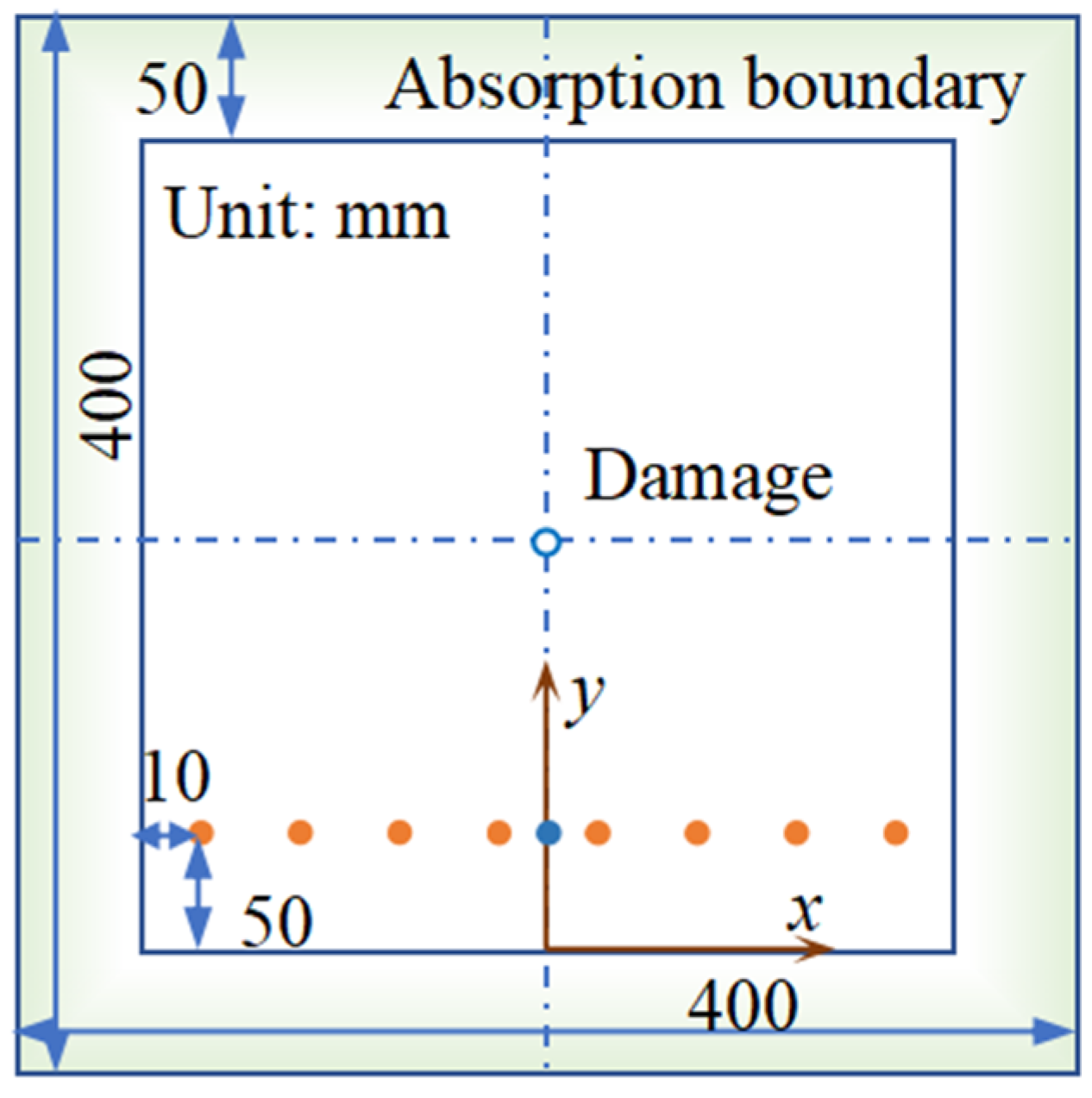
4.1. Finite Element Simulation Model

The proposed method was validated based on a COMSOL 5.6 finite element numerical simulation as shown in Figure 3. The specimen was an aluminum plate with dimensions of 400 × 400 × 2 mm³. The density of the aluminum plate was 2700 kg/m³, the modulus of elasticity was 70 GPa, and the Poisson’s ratio was 0.33. In order to avoid the influence of the reflected waves at the boundaries, a Rayleigh damping absorption condition with a width of 50 mm was set up at the surrounding boundaries of the model. A total of nine array elements were set up; among them, the middle one excited the Lamb wave signal with coordinates of (0, 50) mm and the other eight were used to receive the Lamb wave signal. The longitudinal coordinates of all the array element positions were set to 50 mm, and the transverse coordinates were set from −140 mm at 40 mm intervals to 140 mm. Antisymmetric displacement loads along the thickness direction were applied to excite the A0 mode Lamb wave. Damage was simulated to a through-hole of 5 mm in diameter, with the exact location adjusted according to the research needs. In the finite element simulation model, the meshes near the damage and the transducer unit were refined, with a minimum mesh size of 0.01 mm and a maximum mesh size of 0.15 mm; the initial computational step size was 0.1 μs, and the step size was automatically adjusted with the advancement of the computational process [28]. The excitation signal was a sinusoidal pulse signal modulated by a five-cycle Hanning window with a center frequency of 200 kHz.

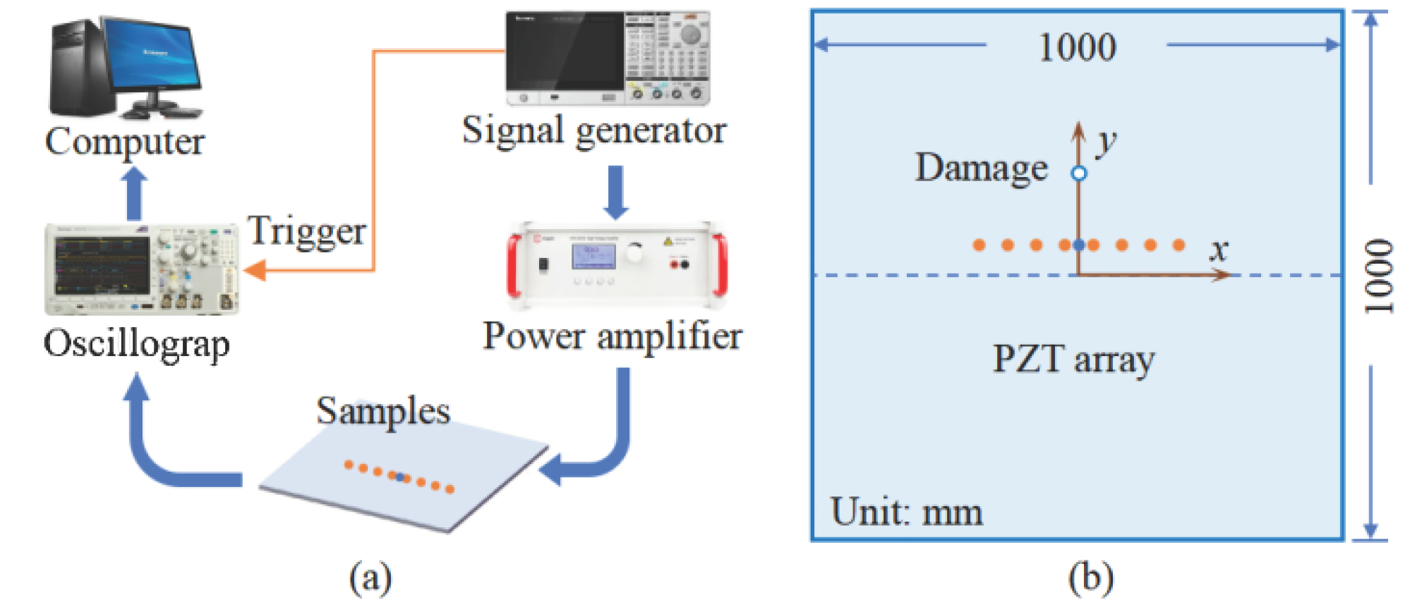
4.2. Construction of Experiment Platform

As shown in Figure 4, an aluminum plate with a length of 1000 mm, width of 1000 mm, and thickness of 2 mm was used in the experiments. The mechanical parameters of the material were the same as those used in the numerical simulation part. A uniform linear array of N = 9 PZT array elements was glued in the plate at positions consistent with the simulation coordinates, and the dimensions of the PZTs were Φ7 mm × 0.5 mm, numbered from left to right from 1 to 9. The damage was simulated with a magnet with a diameter of 5 mm, whose position can be adjusted according to the experimental validation needs.

4.3. Quantitative Metrics of Imaging Results

To compare different imaging methods, two quantitative metrics—the Array Performance Indicator (API) [29] and SNR [30]—were introduced to evaluate the performance of array imaging. The API is a dimensionless parameter that represents the point spread function of the spatial dimension of the image resolution.

$$\mathrm{API}={\displaystyle \frac{S}{{\lambda }^2}}$$

(12)

where S is the area of the region where the point spread function is greater than the threshold amplitude, with its value taken as the cross-sectional area at the normalized amplitude intensity of −6 dB, and λ is the wavelength at the center frequency of the Lamb wave. A smaller API predicts a higher image resolution. The SNR reflects the relationship between the damage signal and the noise signal, characterizing the overall quality of the ultrasound detection image. It is expressed as follows:

$$\mathrm{SNR}=20\cdot \log {\displaystyle \frac{I_{\mathrm{m}\mathrm{a}\mathrm{x}}}{I_{\mathrm{ave}}}}$$

(13)

where I_max is the maximum value of the defective signal and I_ave is the average value of the background noise. A higher SNR indicates better image quality, as it implies a stronger damage signal relative to the noise.

4.4. Dataset Acquisition and Training

As shown in Figure 5, to obtain the network training and testing dataset, 100 simulated damage points (indicated by blue circles) were randomly generated within the area defined by the lower-left coordinate (−100, 100) mm and the upper-right coordinate (100, 200) mm. The dark blue dot at (0, 50) mm represents the excitation signal position, while the other eight light brown dots are the signal reception positions. The training dataset was generated using Equation (11). To satisfy the conditions of the network training input data, the signals of each channel were initially dispersion-compensated, and the resolved signals were obtained using Hilbert transform. Then, a ToFC data block was generated for each simulated damage point in the imaging region, as the channel dimensions took into account both the real and imaginary parts of the signal, resulting in a channel dimension of 16 for the 8 receiver points. The imaging region is within the black dashed line in Figure 5. Since 100 random damage scenarios were simulated, the input data used for the network training consisted of 100 × 8 = 800 data blocks, each with dimensions of 201 × 101 × 16. The target images for training were generated using the MVDR method. The network was implemented in Python 3.7 using Keras with a Tensorflow backend, running on a personal computer with an Nvidia GTX1660 graphics card. The training set and validation set data were split in a ratio of 8:2. During each training epoch, 30 data samples were fed in batches, and the entire training process consisted of 50 epochs.

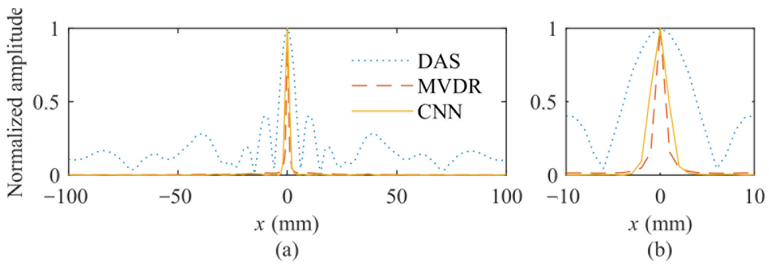
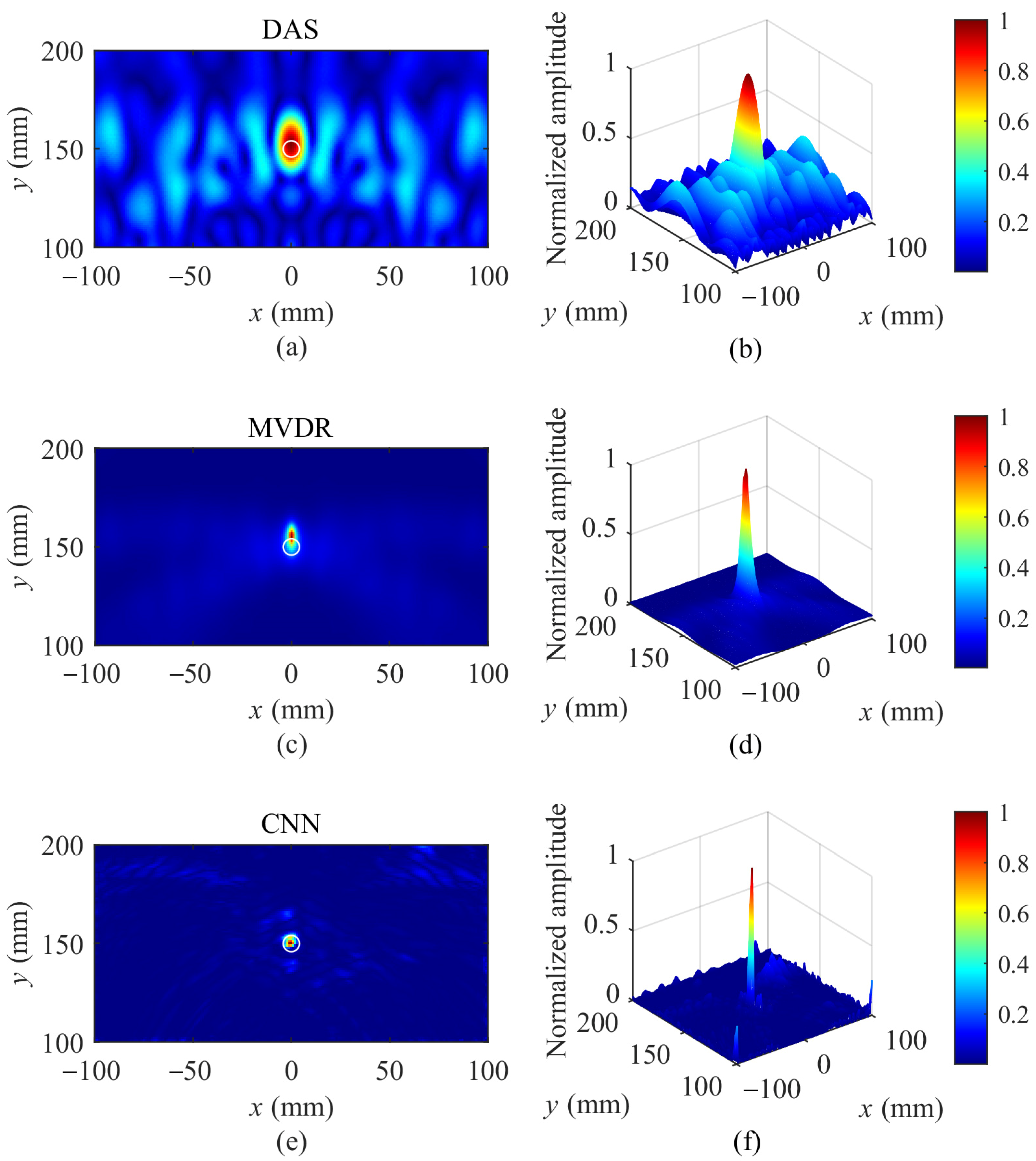
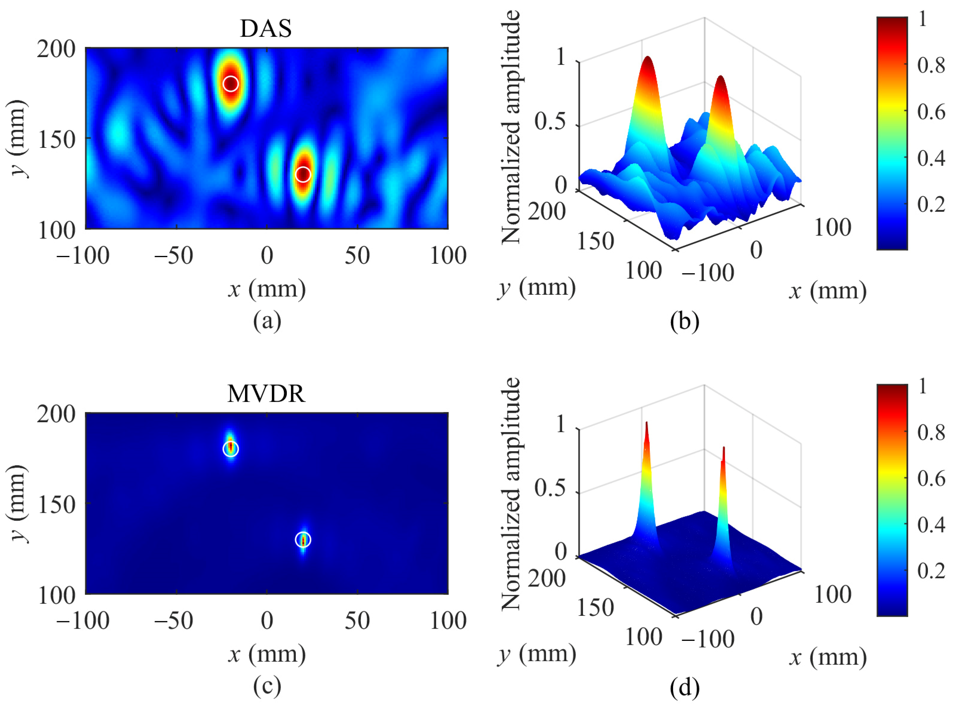
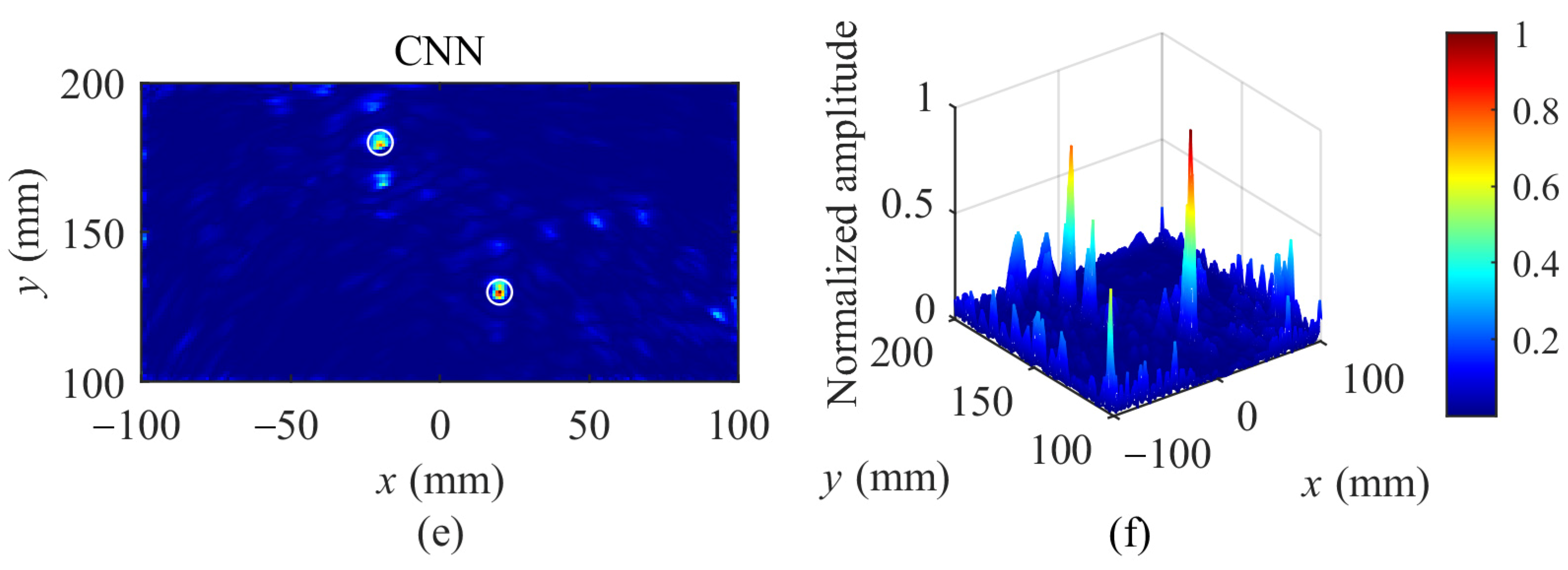
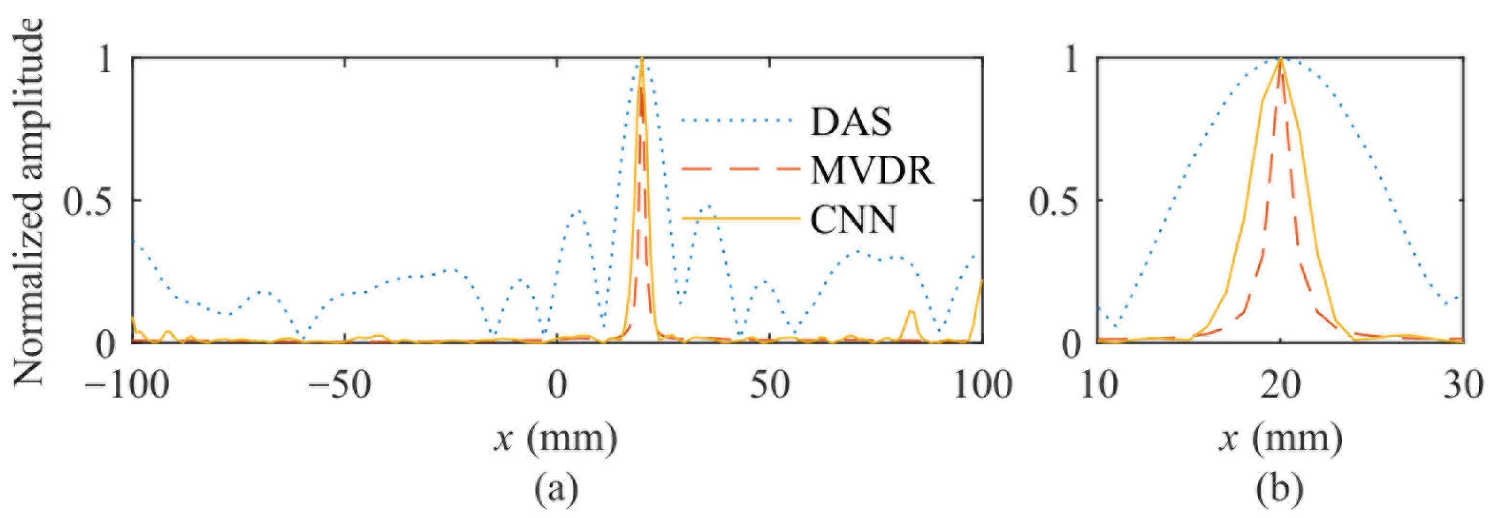
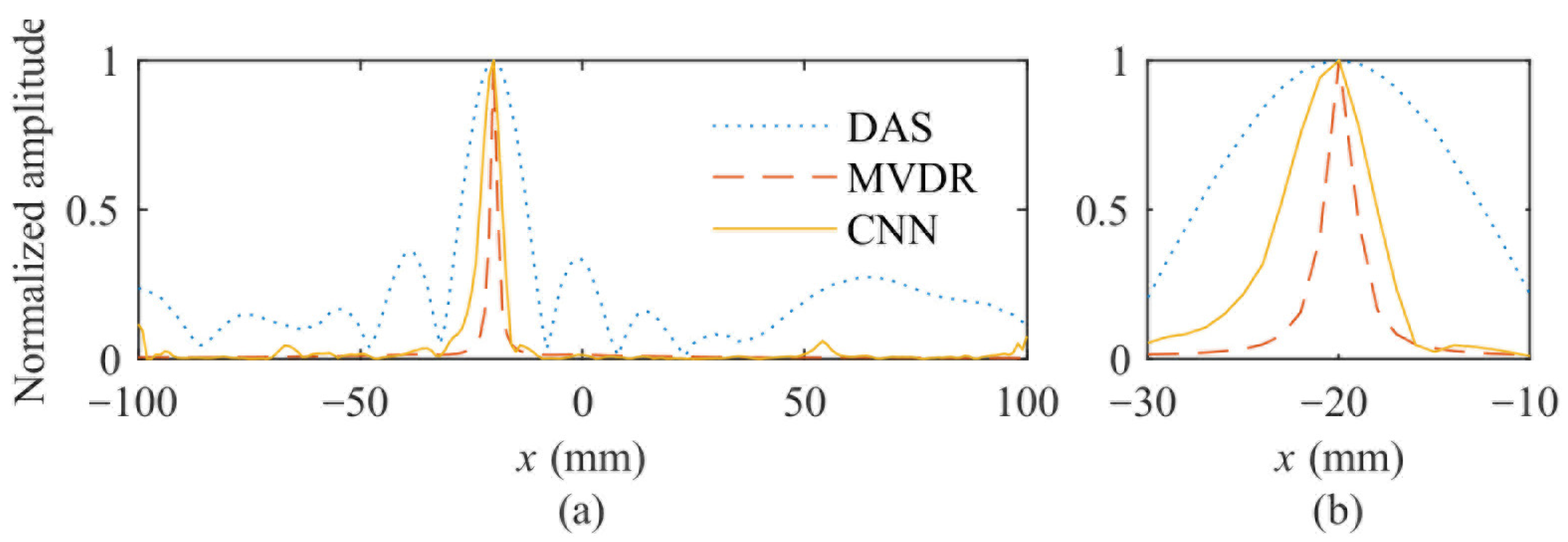
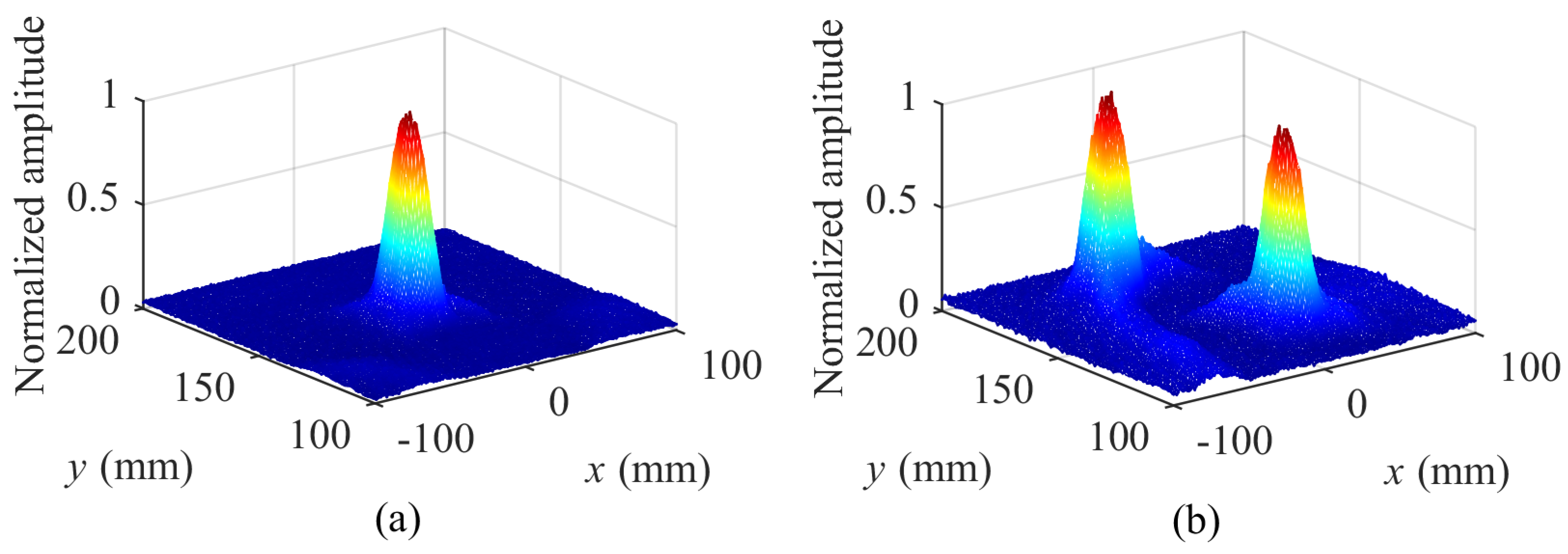
4.5. Simulation Results and Analysis

In order to compare and validate the damage imaging performance of the proposed CNN method, Figure 6 give the imaging results for single damage. Figure 6a,c,e are all 2D planar images of the imaging, while (b), (d), and (f) are the corresponding 3D images; (a) and (b) correspond to the DAS method, (c) and (d) correspond to the MVDR method, and (e) and (f) correspond to the CNN method. The magnitudes of the results in the figures are normalized by their respective maxima, and the damage locations are marked by white circles.

A comparative analysis of the imaging results shown in Figure 6a,c,e reveals that all three methods achieved accurate damage localization. However, the damage area identified by the DAS method exhibited a notably larger spatial extent beyond the marked boundaries, whereas the damage regions reconstructed by both the MVDR and CNN methods were confined within the marked boundaries. As demonstrated in the 3D intensity distributions (Figure 6b,d,f), the MVDR and CNN methods produced significantly sharper focal peaks compared to the DAS method. Specifically, the MVDR results were nearly noise-free, while the CNN method introduced minimal noise—both of which were substantially lower than the noise levels observed in the DAS results. These findings indicate that the proposed CNN-based method achieved imaging performance comparable to the MVDR method and significantly outperformed the DAS method. The CNN framework effectively suppressed most background noise in the images, resulting in a more compact and precise representation of the damage region.

Quantitative comparisons from

Table 1. Quantitative analysis and comparison of evaluation metrics for simulated imaging results.

DAMAGE LOCATION (mm)	API			SNR (dB)
	DAS	MVDR	CNN	DAS	MVDR	CNN
(0, 150)	36.50	2.32	4.16	19.58	121.12	95.62
(−20, 180)	38.26	2.62	4.68	21.41	120.28	89.08
(20, 130)	35.32	2.26	5.03	20.35	119.53	93.16

indicate that the MVDR method achieved the smallest API and the highest SNR. Specifically, the CNN method achieved an API that was approximately one-ninth that of the DAS method, with an SNR that was about 70 dB higher.

To further compare the results of the three methods, the pixel intensity profiles along the horizontal line at the pre-damaged position y = 150 mm are plotted in Figure 7. The comparison shows that all three methods achieved their maximum values at x = 0 mm, confirming that the damage localization accurately corresponded to the pre-damaged position. However, both the CNN and MVDR methods exhibited sharper amplitude distribution curves, indicating that the CNN method had a narrower main lobe width and lower side lobe levels compared to the DAS method. Therefore, the CNN method outperformed the DAS method in terms of narrowing the main lobe width, suppressing background noise, and reducing side lobe levels.

Figure 8 presents the dual-damage imaging results, demonstrating that all three methods accurately identified and localized the two damages. Similar to the single-damage scenario, the damage areas reconstructed by the DAS method (Figure 8a) extended beyond the marked boundaries, whereas those from the MVDR and CNN methods (Figure 8c,e) remain confined within the marked regions. This distinction was further corroborated by the sharpness of the peaks in the 3D intensity profiles (Figure 8b,d,f), where the MVDR and CNN results exhibited significantly narrower focal lobes compared to the DAS. Notably, while the presence of two damages introduced increased noise in Figure 8b (DAS) and Figure 8f (CNN), the MVDR results (Figure 8d) maintained nearly noise-free imaging quality. These observations confirm that the CNN method outperformed DAS in noise suppression and spatial precision but did not yet achieve the robustness of MVDR in fully eliminating interferences between multiple damage signals. From the quantitative comparison in Table 1, it is evident that the API and SNR values obtained using the CNN method were similar to those of the single damage scenario. This similarity was further verified by examining the amplitude contours along the horizontal line at the location of the two injuries, as shown in Figure 9 and Figure 10. The CNN method exhibited a narrower main lobe width and lower side lobe levels compared to the DAS method. The results show that the MVDR method can effectively suppress the interference of the damage signals with each other, and the CNN method, although it reduces the noise level compared with the DAS method, is still affected by the interference between the damage signals and is not yet able to achieve the performance of MVDR.

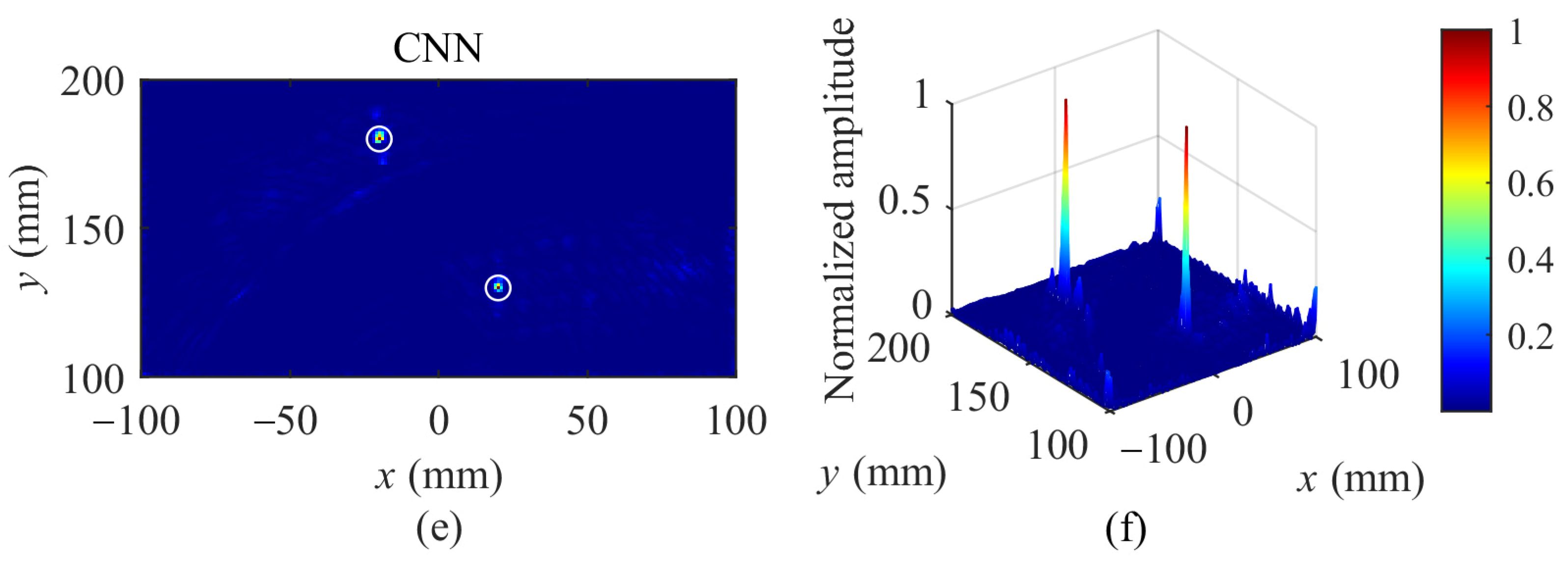
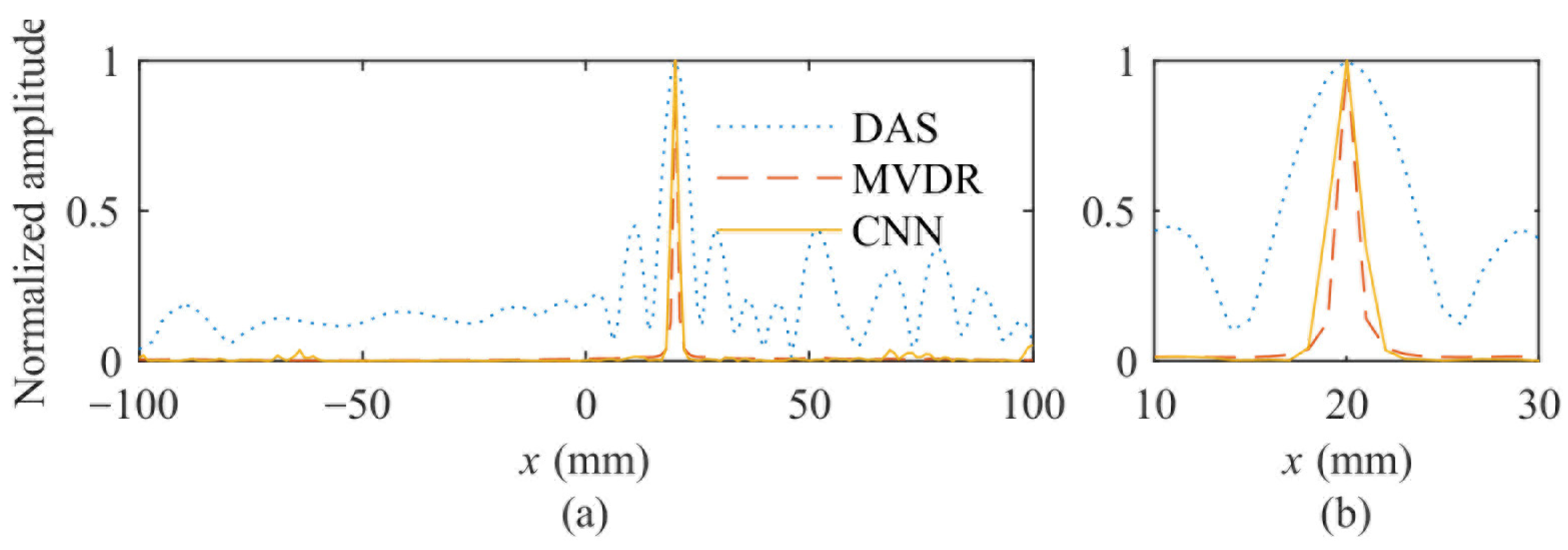
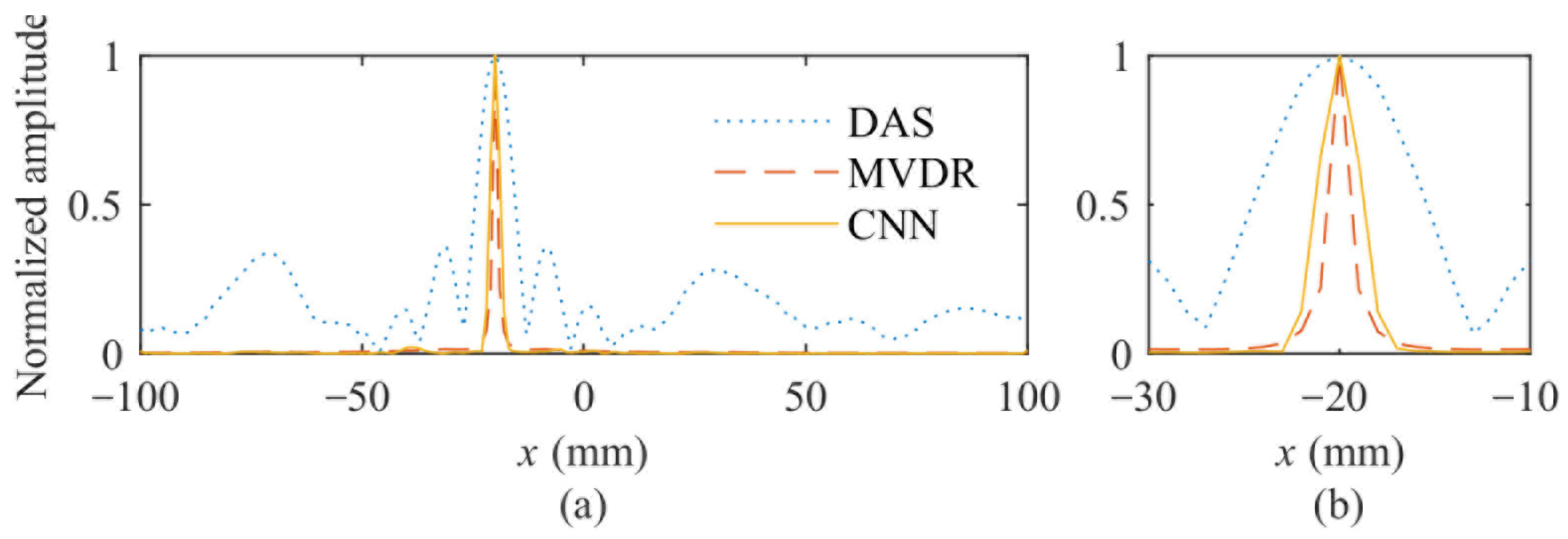
4.6. Experimental Results and Analysis

Consistent with the damage locations set in the simulation model, PZT unit No. 5 in the middle was used to generate the Lamb wave, while the other eight PZTs received the Lamb wave signals and collected experimental data under both single-damage and double-damage conditions. The numbering and arrangement in these figures are consistent with the simulation results, and the quantitative comparison of API and SNR values is provided in

Table 2. Quantitative analysis and comparison of evaluation metrics for experimental imaging results.

DAMAGE LOCATION (mm)	API			SNR (dB)
	DAS	MVDR	CNN	DAS	MVDR	CNN
(0, 150)	25.82	4.13	8.18	16.44	82.32	54.81
(−20, 180)	28.16	3.96	7.72	15.97	73.08	57.16
(20, 130)	26.36	4.08	7.69	15.85	70.29	55.38

.

The experimental single-damage imaging results are illustrated in Figure 11. Consistent with the simulation findings, all three methods achieved accurate damage localization within the marked boundaries (Figure 11a,c,e). The damage regions reconstructed by MVDR and CNN (Figure 11d,f) exhibited sharper intensity profiles compared to the DAS (Figure 11b). However, due to experimental noise in the acquired signals, the imaging noise levels increased across all methods. Notably, even the MVDR results (Figure 11d) showed slightly elevated noise compared to their simulated counterparts (Figure 6d). A quantitative analysis confirms that the CNN method effectively suppresses most background noise relative to the DAS method, yielding a more compact damage representation. This was further validated by the transverse intensity profiles at y = 150 mm (Figure 12), where the CNN demonstrated a sharper amplitude distribution than the DAS.

For dual-damage imaging (Figure 13), all three methods accurately identified and localized both damages (Figure 13a,c,e). The sharpness of MVDR and CNN results (Figure 13d,f) remained superior to those of the DAS (Figure 13b), though noise in the CNN output (Figure 13f) slightly exceeded that of the MVDR (Figure 13d). These observations were corroborated by the transverse intensity profiles at the two damage locations (Figure 14 and Figure 15). Quantitative metrics in Table 2 revealed that, for both single- and dual-damage cases, the API values obtained by DAS were approximately four times higher than those of CNN, while the SNR of DAS was approximately 40 dB lower. These results collectively demonstrate that the CNN method achieves narrower main lobe widths and lower side lobe levels compared to DAS, significantly enhancing imaging resolution and noise robustness.

Figure 16 presents the three-dimensional imaging results obtained using the FCNN method [24], based on experimental single- and dual-damage datasets. The results demonstrated that the FCNN method achieved accurate damage identification and localization. However, a comparative analysis between Figure 16a,b, Figure 11f and Figure 13f revealed that the main lobes of the damage regions reconstructed by the FCNN method were significantly broader than those generated by the proposed CNN method. This indicates that the FCNN-based imaging yielded larger damage areas, thereby reducing imaging resolution. In contrast, the CNN method produced a more compact damage representation, which enhanced spatial resolution. Furthermore, while both methods suppressed background noise to some extent, the CNN method exhibited noise in multi-damage scenarios (Figure 13f), suggesting that further improvements in noise suppression are required to fully mitigate the interference between damage signals.

Through the analysis of both simulation and experimental imaging results, it is evident that the proposed CNN-based adaptive beamforming method effectively improves Lamb wave damage imaging. Compared to the DAS imaging method, the CNN method produces images with a narrower main lobe and lower side lobe levels, thereby enhancing imaging resolution and significantly reducing background noise. This demonstrates the effectiveness of the CNN method in achieving higher-quality damage imaging.

The proposed framework not only improves the SNR and computational efficiency but also exhibits strong potential for real-time SHM applications, owing to its rapid weight prediction capability. However, certain limitations warrant further investigation. Specifically, the method’s performance on complex structures and scenarios involving multiple damage types requires additional validation. Furthermore, optimizing the model’s generalizability will necessitate the incorporation of more diverse experimental datasets to address potential domain shifts in practical implementations.

5. Conclusions

A deep-learning-based improved Lamb wave adaptive DAS beamforming imaging method is proposed. This method employs a compact, CNN-model-based beamforming architecture that significantly enhances the speed, resolution, and SNR of Lamb wave damage imaging. The CNN method directly maps the delayed Lamb wave input signals from each channel into adaptive beamforming weight vectors through the network model, avoiding the need for the inverse calculation of weight vectors by inverting the covariance matrix of the delayed signals, as required in the MVDR method.

Through numerical simulations and experiments, single and double damages in aluminum plates were imaged using the proposed CNN-weighted adaptive DAS beamforming method, as well as the traditional DAS and MVDR methods. A comparative analysis was conducted on the quality of damage imaging, transverse damage index profiles at the damage sites, and quantitative comparisons of the API and SNR. The results show that the resolution and SNR of the CNN-based method can approach or match those of the MVDR method, while being significantly better than those of the DAS method. Specifically, the CNN-based method exhibits a narrower main lobe width and lower side lobe levels, with superior quantitative metrics, such as those of API and SNR, compared to the DAS method. In the experiments with three preset damages, the CNN method achieved an API that was only one-third of that obtained by the DAS method, while also attaining an SNR nearly 40 dB higher than that of the DAS method. Since the constructed CNN network establishes a nonlinear mapping relationship between the input and the output during the training stage, the trained model can quickly predict the weighting parameter for various channels during the testing stage.

The CNN-based adaptive Lamb wave beamforming technique effectively addresses the computational inefficiency and real-time challenges of conventional MVDR methods, whilst preserving high-resolution and high-SNR imaging capabilities. This advancement facilitates rapid, precise damage imaging, thereby enhancing real-time SHM efficacy. Despite achieving a notable balance between imaging efficiency and quality, the proposed CNN approach currently underperforms compared to the MVDR method in imaging quality. Future research will focus on expanding the model’s application to complex structures and analyzing how model architecture and parameter choices affect imaging quality, with the goal of improving the imaging results’ SNR and API.

References

1. Su, Z.; Ye, L. Identification of Damage Using Lamb Waves: From Fundamentals to Applications; Springer Science & Business Media: Berlin/Heidelberg, Germany, 2009; Volume 48. [Google Scholar]
2. Mitra, M.; Gopalakrishnan, S.J. Guided wave based structural health monitoring: A review. Smart Mater. Struct. 2016, 25, 053001. [Google Scholar] [CrossRef]
3. Shan, S.; Qiu, J.; Zhang, C.; Ji, H.; Cheng, L.J. Multi-damage localization on large complex structures through an extended delay-and-sum based method. Struct. Health Monit. 2016, 15, 50–64. [Google Scholar] [CrossRef]
4. Hua, J.; Zhang, H.; Miao, Y.; Lin, J.J. Modified minimum variance imaging of Lamb waves for damage localization in aluminum plates and composite laminates. NDT & E Int. 2022, 125, 102574. [Google Scholar]
5. Liu, Z.; Sun, K.; Song, G.; He, C.; Wu, B.J. Damage localization in aluminum plate with compact rectangular phased piezoelectric transducer array. Mech. Syst. Signal Process. 2016, 70, 625–636. [Google Scholar] [CrossRef]
6. Zhang, S.; Li, C.M.; Ye, W.J. Damage localization in plate-like structures using time-varying feature and one-dimensional convolutional neural network. Mech. Syst. Signal Process. 2021, 147, 107107. [Google Scholar] [CrossRef]
7. Yu, L.; Giurgiutiu, V.J. In-situ optimized PWAS phased arrays for Lamb wave structural health monitoring. J. Mech. Mater. Struct. 2007, 2, 459–487. [Google Scholar]
8. Veidt, M.; Ng, C.; Hames, S.; Wattinger, T.J. Imaging laminar damage in plates using Lamb wave beamforming. Adv. Mater. Res. 2008, 47, 666–669. [Google Scholar] [CrossRef]
9. Sharif-Khodaei, Z.; Aliabadi, M.J. Assessment of delay-and-sum algorithms for damage detection in aluminum and composite plates. Smart Mater. Struct. 2014, 23, 075007. [Google Scholar] [CrossRef]
10. Tian, Z.; Howden, S.; Ma, Z.; Xiao, W.; Yu, L. Pulsed laser-scanning laser Doppler vibrometer (PL-SLDV) phased arrays for damage detection in aluminum plates. Mech. Syst. Signal Process. 2019, 121, 158–170. [Google Scholar] [CrossRef]
11. Michaels, J.E.; Hall, J.S.; Michaels, T.E. Adaptive imaging of damage from changes in guided wave signals recorded from spatially distributed arrays. In Proceedings of the Health Monitoring of Structural and Biological Systems 2009, San Diego, CA, USA, 9–12 March 2009; pp. 351–361. [Google Scholar]
12. Hall, J.S.; Michaels, J.E. Minimum variance ultrasonic imaging applied to an in situ sparse guided wave array. IEEE Trans. Ultrason. Ferroelectr. Freq. Control. 2010, 57, 2311–2323. [Google Scholar] [CrossRef]
13. Engholm, M.; Stepinski, T.J. Adaptive beamforming for array imaging of plate structures using lamb waves. IEEE Trans. Ultrason. Ferroelectr. Freq. Control. 2010, 57, 2712–2724. [Google Scholar] [CrossRef] [PubMed]
14. Hua, J.; Lin, J.; Zeng, L.; Luo, Z.J. Minimum variance imaging based on correlation analysis of Lamb wave signals. Ultrasonics 2016, 70, 107–122. [Google Scholar]
15. Xu, C.; Yang, Z.; Zuo, H.; Deng, M. Minimum variance Lamb wave imaging based on weighted sparse decomposition coefficients in quasi-isotropic composite laminates. Compos. Struct. 2021, 275, 114432. [Google Scholar]
16. Peng, L.; Xu, C.; Gao, G.; Hu, N.; Deng, M. Lamb wave based damage imaging using an adaptive Capon method. Meas. Sci. Technol. 2023, 34, 125406. [Google Scholar] [CrossRef]
17. Perfetto, D.; De Luca, A.; Perfetto, M.; Lamanna, G.; Caputo, F. Damage detection in flat panels by guided waves based artificial neural network trained through finite element method. Materials 2021, 14, 7602. [Google Scholar] [CrossRef]
18. Humer, C.; Höll, S.; Kralovec, C.; Schagerl, M. Damage identification using wave damage interaction coefficients predicted by deep neural networks. Ultrasonics 2022, 124, 106743. [Google Scholar] [CrossRef]
19. Ma, J.; Hu, M.; Yang, Z.; Yang, H.; Ma, S.; Xu, H.; Yang, L.; Wu, Z.J. An efficient lightweight deep-learning approach for guided Lamb wave-based damage detection in composite structures. Appl. Sci. 2023, 13, 5022. [Google Scholar] [CrossRef]
20. Su, C.; Jiang, M.; Lv, S.; Lu, S.; Zhang, L.; Zhang, F.; Sui, Q.J. Improved damage localization and quantification of CFRP using Lamb waves and convolution neural network. IEEE Sens. J. 2019, 19, 5784–5791. [Google Scholar] [CrossRef]
21. Song, H.; Yang, Y.J. Super-resolution visualization of subwavelength defects via deep learning-enhanced ultrasonic beamforming: A proof-of-principle study. NDT E Int. 2020, 116, 102344. [Google Scholar] [CrossRef]
22. Zhang, B.; Hong, X.; Liu, Y.J. Deep convolutional neural network probability imaging for plate structural health monitoring using guided waves. IEEE Trans. Instrum. Meas. 2021, 70, 2510610. [Google Scholar]
23. Wang, X.; Li, J.; Wang, D.; Huang, X.; Liang, L.; Tang, Z.; Fan, Z.; Liu, Y.J. Sparse ultrasonic guided wave imaging with compressive sensing and deep learning. Mech. Syst. Signal Process. 2022, 178, 109346. [Google Scholar] [CrossRef]
24. Shen, R.H.; Zhou, Z.X.; Xu, G.D.; Zhang, S.; Xu, C.G.; Xu, B.Q.; Luo, Y. Adaptive Weighted Damage Imaging of Lamb Waves Based on Deep Learning. IEEE Access 2024, 12, 128860–128870. [Google Scholar] [CrossRef]
25. Sternini, S.; Pau, A.; Di Scalea, F.L. Minimum-variance imaging in plates using guided-wave-mode beamforming. IEEE Trans. Ultrason. Ferroelectr. Freq. Control. 2019, 66, 1906–1919. [Google Scholar]
26. Haskins, G.; Kruger, U.; Yan, P. Deep learning in medical image registration: A survey. Mach. Vis. Appl. 2020, 31, 8. [Google Scholar]
27. Wei, A.; Guan, S.; Wang, N.; Lv, S. Damage detection of jacket platforms through improved stacked autoencoder and softmax classifier. Ocean. Eng. 2024, 306, 118036. [Google Scholar] [CrossRef]
28. Xu, B.Q.; Shen, Z.H.; Ni, X.W.; Wang, J.J.; Guan, J.F.; Lu, J. Thermal and mechanical finite element modeling of laser-generated ultrasound in coating–substrate system. Opt. Laser Technol. 2006, 38, 138–145. [Google Scholar]
29. Zhang, J.; Drinkwater, B.W.; Wilcox, P.D. Effects of array transducer inconsistencies on total focusing method imaging performance. NDT & E Int. 2011, 44, 361–368. [Google Scholar]
30. Velichko, A.; Wilcox, P.D. An analytical comparison of ultrasonic array imaging algorithms. J. Acoust. Soc. Am. 2010, 127, 2377–2384. [Google Scholar]
Figure 1. Workflow from delay compensated data to damage imaging in conventional and CNN based beamformers.
Applsci 15 03801 g001
Figure 2. The proposed CNN network architecture.
Applsci 15 03801 g002
Figure 3. Finite element simulation model of a 9-element linear array.
Applsci 15 03801 g003
Figure 4. (a) Diagram of the experimental setup; (b) Schematic of the plate, piezoelectric array, and damage.
Applsci 15 03801 g004
Figure 5. Simulated 100 random damage locations.
Applsci 15 03801 g005
Figure 6. Imaging results of three imaging methods on single-damage simulation data: (a) DAS, 2D, (b) DAS, 3D, (c) MVDR, 2D, (d) MVDR, 3D, (e) CNN, 2D, (f) CNN, 3D.
Applsci 15 03801 g006
Figure 7. Transverse damage index profiles at y = 150 mm for different imaging methods based on simulation data: (a) full view, (b) zoom-in view.
Applsci 15 03801 g007
Figure 8. Imaging results of three imaging methods on dual-damage simulation data: (a) DAS, 2D, (b) DAS, 3D, (c) MVDR, 2D, (d) MVDR, 3D, (e) CNN, 2D, (f) CNN, 3D.
Applsci 15 03801 g008aApplsci 15 03801 g008b
Figure 9. Transverse damage index profiles at y = 130 mm for different imaging methods based on simulation data: (a) full view, (b) zoom-in view.
Applsci 15 03801 g009
Figure 10. Transverse damage index profiles at y = 180 mm for different imaging methods based on simulation data: (a) full view, (b) zoom-in view.
Applsci 15 03801 g010
Figure 11. The imaging results of three imaging methods on single-damage experimental data: (a) DAS, 2D, (b) DAS, 3D, (c) MVDR, 2D, (d) MVDR, 3D, (e) CNN, 2D, (f) CNN, 3D.
Applsci 15 03801 g011
Figure 12. Transverse damage index profiles at y = 150 mm for different imaging methods based on experimental data: (a) full view, (b) zoom-in view.
Applsci 15 03801 g012
Figure 13. The imaging results of three imaging methods on double-damage experimental data: (a) DAS, 2D, (b) DAS, 3D, (c) MVDR, 2D, (d) MVDR, 3D, (e) CNN, 2D, (f) CNN, 3D.
Applsci 15 03801 g013aApplsci 15 03801 g013b
Figure 14. Transverse damage index profiles at y = 130 mm for different imaging methods based on experimental data: (a) full view, (b) zoom-in view.
Applsci 15 03801 g014
Figure 15. Transverse damage index profiles at y = 180 mm for different imaging methods based on experimental data: (a) full view, (b) zoom-in view.
Applsci 15 03801 g015
Figure 16. FCNN-based damage imaging (experimental data): (a) single damage, (b) double damage.
Applsci 15 03801 g016