Coordination in Emergency Response System Design: An Application to Hazardous Materials Transportation

Featured Application

Mitigation of the public safety risks associated with dangerous goods shipments.

Abstract

Emergency response, in most cases, requires the coordination of multiple teams often including the emergency medical technicians, the fire fighters, and the police. Although there is a well-established literature on designing emergency response networks, the need to coordinate the multiple resources involved in this effort is largely overlooked. Such coordination requires not only the response time of each resource to the emergency, but the amount of time the teams may have to wait for each other. In this paper, we present a mathematical model for the two-resource maximal covering problem, and devise a genetic algorithm for solving large-scale problem instances. We provide a case study focusing on designing the response to hazardous materials incidents in Chengdu City, China. Our numerical experiments highlight the possibility of improving the current situation by merely reallocating the ambulance and emergency stations to different population zones. We also demonstrate how drastic improvements can be achieved by the establishment of new response facilities.

1. Introduction

Ensuring public safety requires preparedness for a variety of emergencies. These include traffic accidents, medical emergencies, search and rescue operations, terrorist attacks, structure fires, and industrial accidents. Natural disasters, such as wildfires, flooding, earthquakes, hurricanes, and tornados also require appropriate emergency response planning. The initial response to such emergencies is almost always carried out by local authorities, including the police, emergency medical technicians (EMTs) and fire fighters. In case of larger-scale disasters or when specialized response teams are required, such as hazardous material (hazmat) releases, assistance from regional and federal authorities may become necessary. In the U.S., the Incident Command System constitutes a standardized approach to the command, control, and coordination of emergency response providing a common hierarchy within which responders from multiple agencies can be effective [1]. In Canada, the National Emergency Response System enables coordinated efforts in responding to emergencies [2]. For example, in Ontario, the provincial resources to respond to the chemical, biological, radiological, nuclear, or explosive incidents are clearly stated in [3]. Teams from the Windsor, Toronto, and Ottawa fire departments are available to respond to these incidents at the technician level, whereas six smaller cities have committed to make teams available at the operations level for such emergencies.

The efficient deployment and coordination of services, agencies and personnel to provide the earliest possible response to an emergency is crucial for reducing its undesirable effect on the people and the environment. One of the factors that determine the timing of the response is the location, where the various emergency response resources are stationed. The presence of all these teams at the site of an emergency is often required to ensure the effectiveness of the response. Despite the need for coordination, the operations research literature focuses on the location of a single response resource, e.g., ambulance stations or fire stations (see Section 2 for an overview). In this paper, we address this gap in the literature by studying the design of an emergency response network that comprises multiple specialty teams that need to attend the incident simultaneously. Of course, each team can undertake a few activities at the incident site before the others arrive, which could be included in an operational level plan. We adopt a strategic perspective in this paper and aim at maximizing the time the specialty teams can jointly respond to the emergency.

One of the proxies that can be used for measuring the level of coordination among different response teams is the time between their arrival at the scene of emergency. Since the skills, expertise, and equipment of all the teams are needed for an effective response, lower wait times would indicate higher levels of coordination. Traditionally, a possible emergency site is considered “covered” by a response facility, if it is within a predetermined distance (or time) from the facility. The maximum covering location problem, first introduced by [4], can be considered as the basic building block of emergency response network design. The problem involves determining the locations of a given number of response facilities to maximize the number of people who would receive the services of the response team in a timely fashion. In this paper, we present a formulation for the maximal covering problem with two resources, where the concept of coverage is expanded to include an acceptable wait time as well as a desirable response time for each of the teams. Note that this conceptual framework would also apply for the problem with more than two resources, albeit the arising formulation would be more tedious due to the higher dimensionality of the response times and wait times discussed in Section 3.

We apply the proposed methodology for studying the hazmat incident response network in Chengdu City, China. With a population of over 10 million, Chengdu’s urban road network comprises about 1300 nodes and over 2000 edges. The city is currently served by 62 ambulance stations and 20 fire stations. Clearly, this is a large-scale problem instance, and the proposed model is not amenable to solution with readily available optimization software. Therefore, we developed a genetic algorithm for solving the problem instances in the case study. The algorithm allows for the prioritization of one of the response times or the wait time in identifying the ambulance–fire truck pair that should be serving each possible emergency site. We find that the current performance of the response network in Chengdu can be improved by a reallocation of the response resources, rather than simply assigning the closest resource to each zone. We also develop and assess alternative scenarios to expand the current response network to reduce the response and wait times drastically.

The remainder of this paper is organized as follows. An overview of the most relevant literature is provided in Section 2. We present the conceptual underpinnings of our mathematical model in Section 3. The two-resource maximal covering problem is formulated in Section 4, and an illustrative example is outlined Section 5. For solving large instances of the problem, Section 6 outlines the genetic algorithm we developed. Section 7 provides the application of the proposed methodology for designing a hazmat emergency response network in the city of Chengdu. The concluding remarks and future research directions are provided in Section 8.

2. Literature Review

In this section, we provide a selective overview of the coverage formulations, and the reader is referred to [5] for a comprehensive review.

Table 1. Early covering models in the literature.

Paper	Objective	Coverage Threshold
Daskin (1982, 1983) [6]	Max expected no. of covered nodes	Distance
Hogan and Revelle (1986) [7]	Max the back-up coverage	Distance
Gendreau et al. (1997) [8]	Max the no. of nodes covered twice	Distance
Marianov and Serra (1998) [9]	Max the no. of covered nodes	Waiting time in queue
Gandhi et al. (2001) [10]	Max the no. of covered nodes	Response time
Brotcorne et al. (2003) [11]	Max the no. of covered nodes	Distance
Berman et al. (2003) [12]	Max the no. of covered nodes	Gradual coverage
Galvão et al. (2005) [13]	Max expected no. of covered nodes	Distance
Jia et al. (2007) [14]	Max the no. of covered nodes	Coverage level
Sorensen and Church (2010) [15]	Local reliability	Distance

depicts some of the early work on maximum covering models indicating their objective and coverage threshold representation. It is important to note that all these models focus on the use of a single specialty team for responding to an emergency. The cooperation needed among different types of emergency response resources is not captured by these models.

Ref. [16] focused on random link failures and provide a 0–1 linear optimization model to locate response facilities. Their objective is to maximize the rescue coverage. Ref. [17] presented a multi-objective version of the maximal conditional covering location problem. Their model is applied to the relocation of hierarchical emergency response facilities. Extending their work on gradual coverage, ref. [18] focused on joint partial coverage by aggregating the coverage provided by multiple facilities.

Based on fault tree analysis, ref. [19] analyzed the evolution of emergency incidents. Ref. [20] studied the storage location problem for emergency supply, where the goal is decreasing the cost of response supplies when large-scale emergency response is needed. Emergency evacuation has attracted the attention of some researchers including [21,22,23]. This stream of research is mainly based on simulation modeling and network design, and focuses on traffic flow, scheduling design, traffic signal, traffic routing, the information of timely traffic, and activity behavior. The objectives include designing rapid response strategies, quickly transferring evacuees, and mitigating disaster consequences.

Table 2. Emergency response for hazmat transportation.

Paper	Network				Sub-Problem
	Rural	Highway	Rail	Urban	Covering	Location	Evacuation	Routing
Saccomanno and Allen (1988) [24]	×					×
Berman et al. (2007) [26]		×			×			×
Zografos and Androutsopoulos (2008) [27]	×				×	×	×
Taslimi et al. (2017) [28]		×				×	×	×
Zhao and Ke (2019) [29]				×	×	×
Mohabbati-Kalejahi and Vinel (2021) [30]		×			×	×
Ke (2022) [31]				×		×	×
Wang et al. (2023) [32]			×

provides a comparison of the papers, focusing on hazmat transportation, with regards to the type of transport network considered and the sub-problem involved in the developed model. These papers assume that the hazmat incident will be attended by specialized hazmat response teams. The first model was developed by [24], where the emergency facility is in a rural road network to respond to a spill incident. Since the incident probabilities in this context are very low [25], the rescue teams are assumed always to be available. Ref. [26] assumed a pre-set coverage distance in developing their mathematical model for the arc-covering problem defined on a highway network. Ref. [27] focused on the travel time, evacuation, risk and cost, and optimized location decisions and coverage of response deployment for the hazmat distribution routes. Recently, ref. [28] proposed a bi-level model to design the hazmat transportation network and locates the emergency team based on a road network between specified OD pairs. The average response time was considered to assess the corresponding risk.

During the past five years, there has been renewed interest in hazmat emergency response. Ref. [29] studied the location and capacity of hazardous waste storage sites and the development of emergency response policies. They proposed a bi-level programming model, which is applied to a real-life case from Daojiao city, China. The same case study is used in [31], which proposed a two-stage robust optimization approach for designing an emergency response system. The location and capacity of the emergency response facilities are determined in the first stage, whereas the second stage aims at minimizing the time-varying rescue risk by identifying the optimal resource allocation. Ref. [30] presented a bi-objective formulation where the configurational decisions pertaining to a closed-loop supply chain are optimized simultaneously with the locations of the hazmat emergency response teams. They developed a two-phase methodology to characterize all the solutions on the cost–risk Pareto frontier. Ref. [32] focused on the uncertainties concerning demand, service, scope, and safety parameters in determining the optimal sites for rail emergency response facilities. The authors introduced a robust control safety parameter to represent the risk preferences of the decision maker.

In this paper, we consider the need for multiple types of resources in responding to an emergency. In the context of hazmat transport, we explicitly model the time between the arrival of two different types of emergency response teams at the accident site. This has clear implications concerning the duration of the response to an emergency incident, which has been studied extensively in the empirical literature on transportation using hazard-based duration models. Typically, these models establish a survival function through the link between the hazard function and a duration model, e.g., Weibull, exponential, Log-logistic.

3. Modeling the Response Times

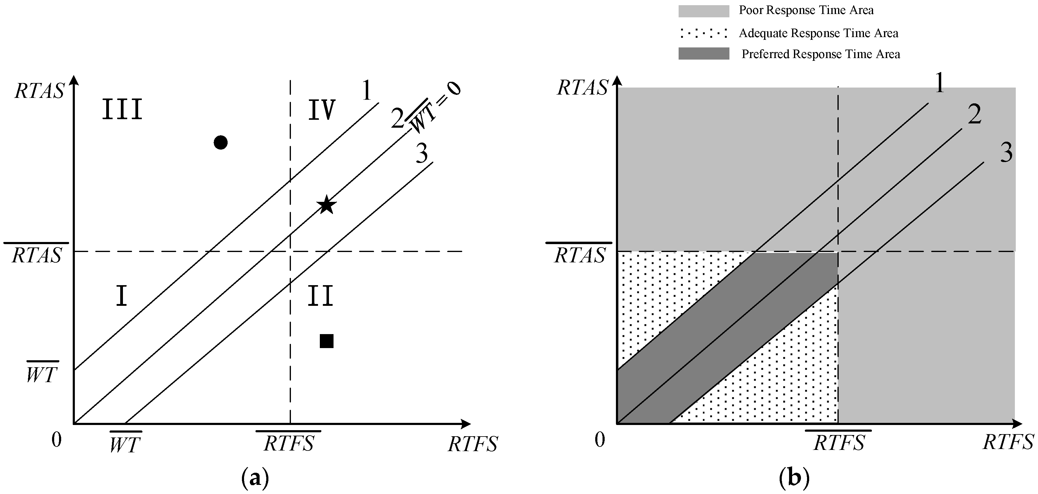
In this section, we focus on emergency response planning with two resources, i.e., fire stations and ambulance stations, for the ease of exposition. Our aim is to lay the groundwork for the mathematical formulation of the problem in the next Section. In the event of an emergency, at any node on the network, the closest fire and ambulance stations will be informed simultaneously, and they will dispatch response teams via the shortest routes to the scene. At any node i, we assume that, if the response time of the fire station (RTFS_i) is greater than the response time of the ambulance station (RTAS_i), then the EMTs will have to wait for the firemen, and vice versa. The amount of time one of the teams would be waiting is WT_i = |RTFS_i − RTAS_i|. Let $\overline{RTFS}$, $\overline{RTAS}$, and $\overline{WT}$ denote the prespecified targets for the response and wait times across the road network.

Figure 1a, where each node is depicted in terms of its (RTFS_i, RTAS_i), enables us to categorize the level of collaboration among the ambulances and firetrucks. Clearly, the highest level of collaboration is when the node is on the 45° line, e.g., the star on line 2 in Figure 1a, where WT_i = 0. The figure is divided into four quadrants using $\overline{RTFS}$ and $\overline{RTAS}$. Line 1 and line 3 have $\overline{WT}$ as intercept and a 45° slope. Thus, WT_i > $\overline{WT}$ at both the circle and the square in Figure 1a, where the firemen wait in the former and the EMTs wait in the latter. The shaded area in Figure 1b depicts the poor, adequate, and preferred response time areas. If a node is in a preferred response time area (dark shaded), then its RTFS_i, RTAS_i, and WT_i are all below their respective targets. By contrast, the light shaded area in Figure 1b represents the poor response time area, where both response times are above their respective targets. We deem the dotted area in Figure 1b to be an adequate response: although the wait time is above its target, the two response times are in the preferable range. The aim is to maximize the number of nodes moved to the preferred response time area by the construction of new ambulance and fire stations.

4. Two-Resource Maximal Covering Model

In this section, we expand the maximal covering problem formulation to capture the presence of two emergency response resources that need to be coordinated. We consider each node on the urban transport network a candidate site for an ambulance and/or fire station. We do not explicitly model the spatial distribution of population density, which amounts to assigning the same priority for covering each node. The response times for each node are calculated for the dispatch of a vehicle from the closest station via the shortest route at an average vehicle speed of 60 km/h. Please see the Abbreviations section at the end of the manuscript for our notation.

Naturally, o_i = 1 for i ∈ EAS and p_i = 1 for i ∈ EFS. In order to capture the coordination between ambulances and fire stations, we define the auxiliary variable as follows:

$$x_{ij}=o_i\times p_j$$

(1)

That is, x_ij = 1 if the ambulance station i and the fire station j are established simultaneously; 0, otherwise. Since x_ij is nonlinear in terms of the decision variables, we will include its linearization in the model below. We now define two parameters that indicate the nodes that will be moved from the poor and adequate response time areas to the preferred response time areas, respectively. The value of A_ijk indicates the nodes that will move from the poor area to the preferred area by the co-establishment of an ambulance station at node i and a fire station at node j. That is, A_ijk: a binary parameter, and each node k ∈ A^Poor, where

$$A_{ijk}=\left\{\begin{array}{l}1 \mathrm{when} x_{ij}=1,\left|D{H}_{ik}-D{F}_{jk}\right|\le \overline{WT}, D{H}_{ik}\le \overline{RTAS}, D{F}_{jk}\le \overline{RTFS}\\ 0 \mathrm{otherwise}\end{array}\right.$$

(2)

Similarly, B_ijl keeps track of the nodes that move from the adequate area to the preferred area by the simultaneous establishment of an ambulance station at node i and a fire station at node j. That is,

B_ijl: a binary parameter, and for each node l ∈ A^Adeq, where

$$B_{ijl}=\left\{\begin{array}{l}1 \mathrm{when} x_{ij}=1,\left|D{H}_{il}-D{F}_{jl}\right|\le \overline{WT}, D{H}_{il}\le \overline{RTAS}, D{F}_{jl}\le \overline{RTFS}\\ 0 \mathrm{otherwise}\end{array}\right.$$

(3)

Mathematical Model

$$\max f={\displaystyle \sum _{k\in A^{Poor}}{y}_k}+{\displaystyle \sum _{l\in A^{Adeq}}{z}_l}$$

(4)

                 subject to

$${\displaystyle \sum _{i\in EAS\cup AAS}{o}_i}\le NA$$

(5)

$${\displaystyle \sum _{j\in EFS\cup AFS}{p}_j}\le NF$$

(6)

$$x_{ij}\le o_i$$

(7)

$$x_{ij}\le p_j$$

(8)

$$x_{ij}\ge o_i+p_j-1$$

(9)

$${\displaystyle \sum _{i\in EAS\cup AAS}{\displaystyle \sum _{j\in EAS\cup AAS}{A}_{ijk}{x}_{ij}}}\ge y_k, \forall k\in A^{Poor}$$

(10)

$${\displaystyle \sum _{i\in EAS\cup AAS}{\displaystyle \sum _{j\in EAS\cup AAS}{B}_{ijl}{x}_{ij}}}\ge z_l, \forall l\in A^{Adeq}$$

(11)

$$x_{ij}\in \{0,1\}, \forall i\in EAS\cup AAS, \forall j\in EFS\cup AFS$$

(12)

$$o_i\in \{0,1\}, \forall i\in AAS$$

(13)

$$p_j\in \{0,1\}, \forall j\in AFS$$

(14)

$$y_k\in \{0,1\}, \forall k\in A^{Poor}$$

(15)

$$z_l\in \{0,1\}, \forall l\in A^{Adeq}$$

(16)

The objective function (4) maximizes the number of nodes in the preferred area after the establishment of the new ambulance and fire stations. It is possible to prioritize the number of nodes in the poor response time area by using a weight for the first term. Constraints (5) and (6) ensure the total number of ambulance stations and fire stations remain within the prespecified limits. Constraints (7)–(9) linearize (1) and ensure that only the established ambulance stations and fire stations can be selected to serve the transportation network. Constraint (10) is a logical constraint for the nodes originally in the poor response time area. It is to keep track of those stations moved to the preferable area when both the response times and the wait time are reduced accordingly. Constraint (11) is a similar logical constraint for the nodes located in the adequate area. The domains the variables are specified by Constraints (12)–(16).

5. Illustrative Example

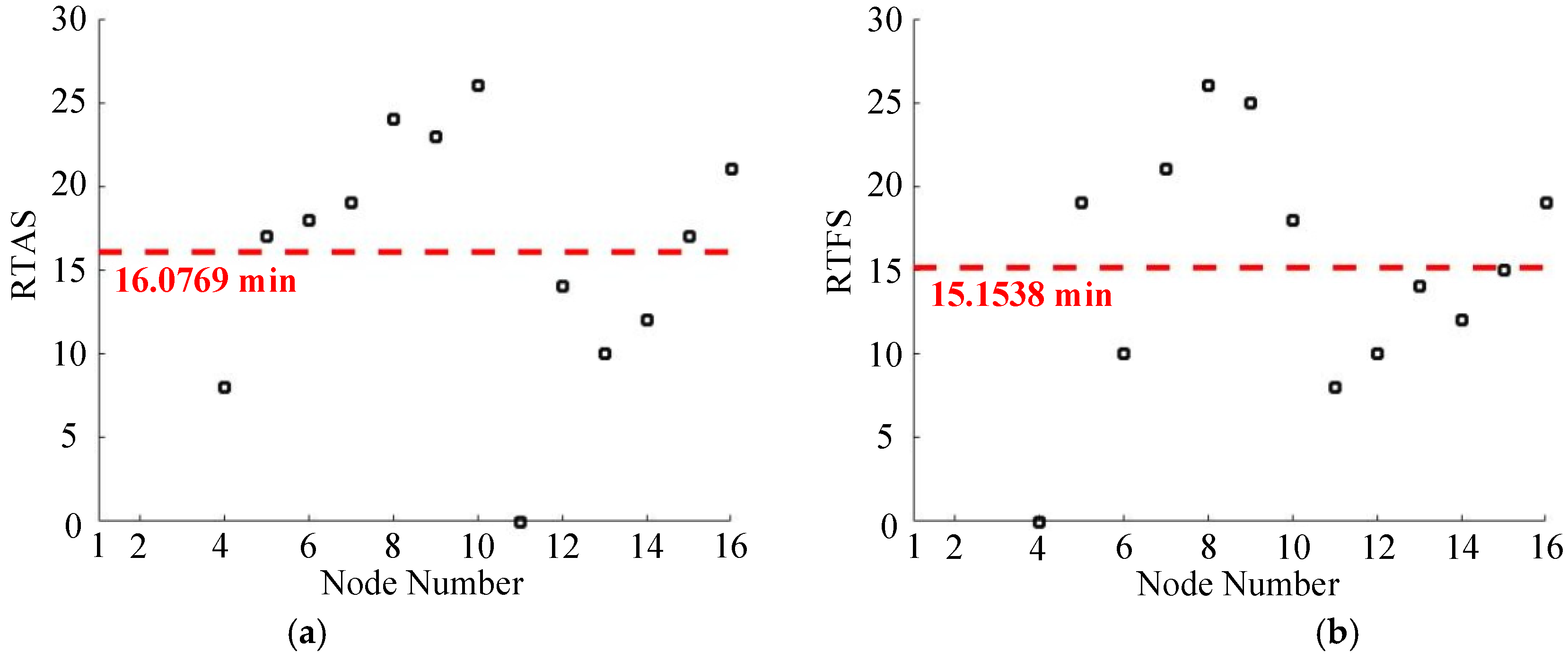
Figure 2 depicts a network, where the locations of an ambulance station and a fire station are also shown. Figure 3 shows the response times for each node in the illustrative example, assuming 60 km/h velocity, as well as their averages, which we use as the targets. Based on these values, the average waiting time is 4 min.

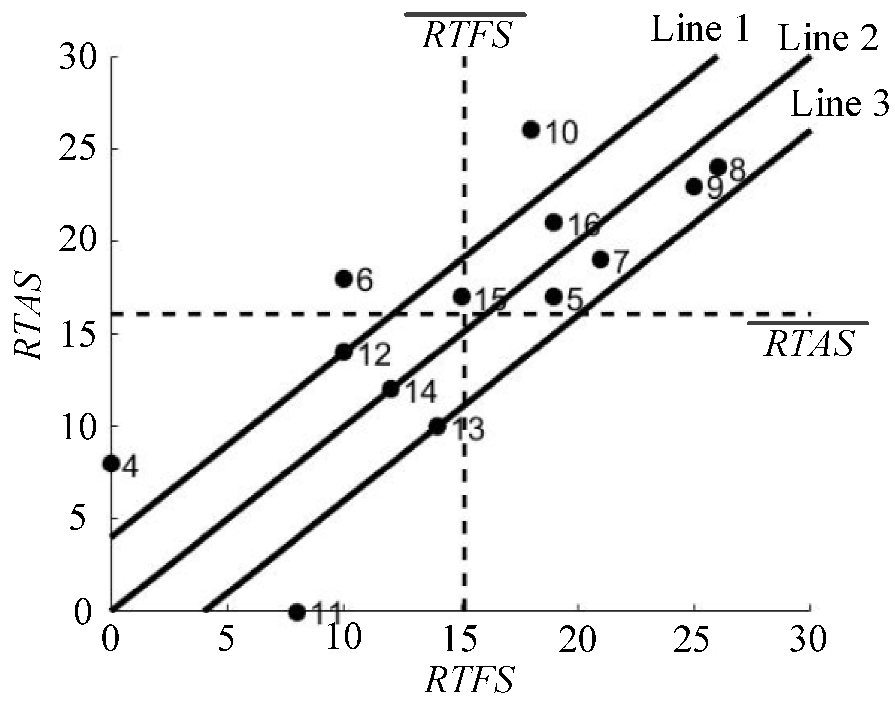
As shown in Figure 4, Nodes 12, 13, and 14 are in the preferred response time area. Nodes 4 and 11, that host one of the existing stations, are in the adequate response time area, since the wait time among the two resources is 8 eight minutes. The rest of the nodes are in the poor response time area.

We solve the proposed model on the active standard platform of CPLEX 12.5 on a computer equipped with 2.40 GHz Inter processor i7-5500U and 8 GB RAM.

Table 3. Optimal solution to the illustrative example.

[NA,NF]	Location		Poor → Pref	Adeq → Pref
	Ambulance Station, oi	Fire Station, pj
[1,1]	i = 11	j = 4	——	——
[1,2]	i = 11	j = 4, 11	——	{4,11}
[2,1]	i = 4, 11	j = 4	{6,15}	{4,11}
[2,2]	i = 7, 11	j = 4, 9	{5,6,7,8,9,10}	——
[2,3]	i = 9, 11	j = 4, 9, 11	{5,6,7,8,9,10}	{4,11}
[3,2]	i = 4, 9, 11	j = 4, 9	{5,6,7,8,9,10,15}	{4,11}
[3,3]	i = 9, 11, 13	j = 4, 7, 13	{5,6,7,8,9,10,15,16}	{4,11}
[4,3]	i = 9, 11, 14	j = 4, 9, 15	{5,6,7,8,9,10,15,16}	{4,11}
[3,4]	i = 9, 11, 14	j = 4, 9, 13	{5,6,7,8,9,10,15,16}	{4,11}
[4,4]	i = 9, 11, 14	j = 4, 9, 13	{5,6,7,8,9,10,15,16}	{4,11}

shows the optimal solution for different [NA, NF] values. (In the remainder of the paper, [.,.] denotes [NA,NF] values referring to the numbers of ambulances and fire stations to be established (existing + new). This is not to be confused by a citation to the list of references, [.].)

It is interesting to note that, when either NA ≥ 3 and NF ≥ 3, the number of the new ambulance and fire stations do not change. Also, although the optimal solution constructs the ambulance and fire stations at different sites, the resulting emergency response is the same as that of NA = 3 and NF = 3, which implies a smaller budget.

6. Genetic Algorithm

In this section, a genetic algorithm will be developed to solve the proposed model for large scale problem instances. Below, we describe the algorithm.

• Setting the Size of the Population: There are two populations. One population consists of the location of ambulance stations. Let NP^AS be the number of ambulance station location populations (ASLP), which means that the number of chromosomes of the ASLP is NP^AS. The other population consists of the location of fire stations (FSLP). Let NP^FS be the number of fire station location populations. The number of chromosomes of the FSLP is NP^FS. The total number of population chromosomes is NP^AS plus NP^FS.
• Coding Scheme of Chromosome: A chromosome consists of genes. Each chromosome of the ASLP has two gene parts. One part is the location of the existing ambulance stations, and the other part is the location of new ambulance stations. The length of the ASLP chromosome is the number of ambulance stations. Every gene of the ASLP chromosome gives the exact location of the ambulance station. The chromosome of the FSLP has the same setting. For instance, as shown in

  Table 4. Parameter setting of the genetic algorithm for an illustrative example.

  The size of ASLP	NPAS = 10
  The size of FSLP	NPFS = 10
  The generation gap	Gap = 0.9
  The crossover probability	pc = 0.9
  The mutation probability	pm = 0.1
  The maximum genetic iteration	100
  The average of RTAS	16.0769 min
  The average of RTFS	15.1538 min
  The average of WT	4.00 min

  , when NA = 3 and NF = 3, the coding scheme of the chromosome is as follows:

ASLP Chromosome Example:	11 |	9 13
FSLP Chromosome Example:	4 |	7 13

The genes left of the vertical line, called Forbidding Crossing Genes, are the location of the existing facilities, and the genes right of the vertical line, called Crossing Genes, are the location of the new facilities. Forbidding Crossing Genes means that the genes cannot be crossed. Crossing Genes means that the genes can be crossed.

3.

Fitness Function: The fitness function is for selecting the outstanding chromosome in the ASLP and FSLP. We consider the number of nodes in the preferred area plus those in the adequate area minus the total number of facilities as the fitness function. It is important to note that there could be more than one ambulance–fire station pair that can be used for moving node k from the poor (or, adequate) zone to the preferred zone. To this end, we consider three user preference options: minimum RTAS, minimum RTFS, and minimum WT. The fitness function and user preferences are as follows:

$$f={\displaystyle \sum _{k\in A^{Poor}}{y}_k}+{\displaystyle \sum _{l\in A^{Adeq}}{z}_l}-\left({\displaystyle \sum _{i\in EAS\cup AAS}{o}_i}+{\displaystyle \sum _{j\in EFS\cup AFS}{p}_j}\right)$$

(17)

Minimum RTAS:

$$\left|D{H}_{ik}-D{F}_{jk}\right|\le \overline{WT}, \min \left(D{H}_{ik}\right)\le \overline{RTAS}, D{F}_{jk}\le \overline{RTFS}$$

(18)

$$\left|D{H}_{il}-D{F}_{jl}\right|\le \overline{WT}, \min \left(D{H}_{il}\right)\le \overline{RTAS}, D{F}_{jl}\le \overline{RTFS}$$

(19)

Minimum RTFS:

$$\left|D{H}_{ik}-D{F}_{jk}\right|\le \overline{WT}, D{H}_{ik}\le \overline{RTAS}, \min \left(D{F}_{jk}\right)\le \overline{RTFS}$$

(20)

$$\left|D{H}_{il}-D{F}_{jl}\right|\le \overline{WT}, D{H}_{il}\le \overline{RTAS}, \min \left(D{F}_{jl}\right)\le \overline{RTFS}$$

(21)

Minimum WT:

$$\min \left(\left|D{H}_{ik}-D{F}_{jk}\right|\right)\le \overline{WT}, D{H}_{ik}\le \overline{RTAS}, D{F}_{jk}\le \overline{RTFS}$$

(22)

$$\min \left(\left|D{H}_{il}-D{F}_{jl}\right|\right)\le \overline{WT}, D{H}_{il}\le \overline{RTAS}, D{F}_{jl}\le \overline{RTFS}$$

(23)

$$\forall i\in EAS\cup AAS, \forall j\in EFS\cup AFS, k\in A^{Poor}, l\in A^{Adeq}$$

(24)

Equation (17) is the fitness function and (24) denotes the domains of i, j, k, and l. Equations (18) and (19) describe the minimum RTAS preference for nodes in the poor and adequate zones, respectively. In this case, the minimum response time of an ambulance station for each node k would be selected when node k could be moved to the preferred zone. Similarly, Equations (20) and (21) describe the minimum RTFS preference, and Equations (22) and (23) describe the minimum WT preference.

4.

Selecting and Crossover: The generation gap is for helping select the outstanding chromosomes and crossing chromosomes. The crossover rules are as follows:

Inside Crossover Rule: The ASLP chromosome crosses the ASLP chromosome with the setting of crossover probability. The FSLP chromosome crosses the FSLP chromosome with the setting of crossover probability.

One to One Crossover Rule: In each crossing, randomly selecting one gene for crossing.

5.

Mutation: The crossing genes can be randomly selected to mutate with mutation probability. The mutation of a gene is to change one location of new facilities into other alternative facility sites except for existing facility sites.

We now apply the genetic algorithm to the illustrative example, which was solved to optimality, in Section 5. The parameter setting of the genetic algorithm is shown in Table 4 and its solution for different values of NA and NF are depicted in

Table 5. Solution with the genetic algorithm.

[NA,NF]	Location		Poor → Pref.	Adeq. → Pref.
	Ambulance Station, oi	Fire Station, pj
[1,1]	i = 11	j = 4	——	——
[1,2]	i = 11	j = 4, 11	——	{4,11}
[2,1]	i = 4, 11	j = 4	{6,15}	{4,11}
[2,2]	i = 7, 11	j = 4, 5	{5,6,7,8,9,10}	——
[2,3]	i = 7, 11	j = 4, 7, 11	{5,6,7,8,9,10}	{4,11}
[3,2]	i = 4, 9, 11	j = 4, 7	{5,6,7,8,9,10,15}	{4,11}
[3,3]	i = 5, 11, 14	j = 4, 7, 12	{5,6,7,8,9,10,15,16}	{4,11}
[4,3]	i = 9, 11, 14	j = 4, 9, 12	{5,6,7,8,9,10,15,16}	{4,11}
[3,4]	i = 7, 11, 12	j = 4, 5, 12	{5,6,7,8,9,10,15,16}	{4,11}
[4,4]	i = 5, 11, 14	j = 4, 5, 13	{5,6,7,8,9,10,15,16}	{4,11}

.

Although the locations of the ambulance and fire stations are different,

Table 6. Parameter setting of the genetic algorithm in the Chengdu case.

The size of ASLP	NPAS = 100
The size of FSLP	NPFS = 100
The generation gap	Gap = 0.9
The crossover probability	pc = 0.9
The mutation probability	pm = 0.1
The maximum genetic iteration	1000

depicts that the collaborative emergency coverage prescribed by the genetic algorithm is the same as the optimal solution in Table 3 (when $\mathrm{NA}\ge$ 2 and $\mathrm{NF}\ge$ 2). Figure 5 shows the solutions of the genetic algorithm under different user preferences. Comparing Figure 5a–c reveal that the response and wait times at Node 6 and Node 4 vary with the user preferences. With the user prioritizing wait times, these two nodes are much closer to line 2, i.e., the zero-wait line.

7. Case Study: Hazmat Transportation in Chengdu City

In this section, we adopt the proposed methodology for improving the collaboration of the fire fighters and EMTs in responding to hazardous materials (hazmat) transport accidents in Chengdu, the capital of China’s Sichuan province (see Figure 6). With a population of more than 10 million, it is the third most crowded city in Western China. Chengdu City has about five thousand companies carrying or stocking hazardous materials.

We first determine the urban road segments that constitute the hazmat transport network (HMTN) of Chengdu. For the ease of exposition, we target avoiding only the primary schools in the urban road network. Then, we apply the genetic algorithm described in the previous section to determine the locations of the ambulance and fire stations so as to maximize the number of nodes collectively covered by these hazmat accident response resources.

7.1. Building the Hazmat Transport Network for Chengdu City

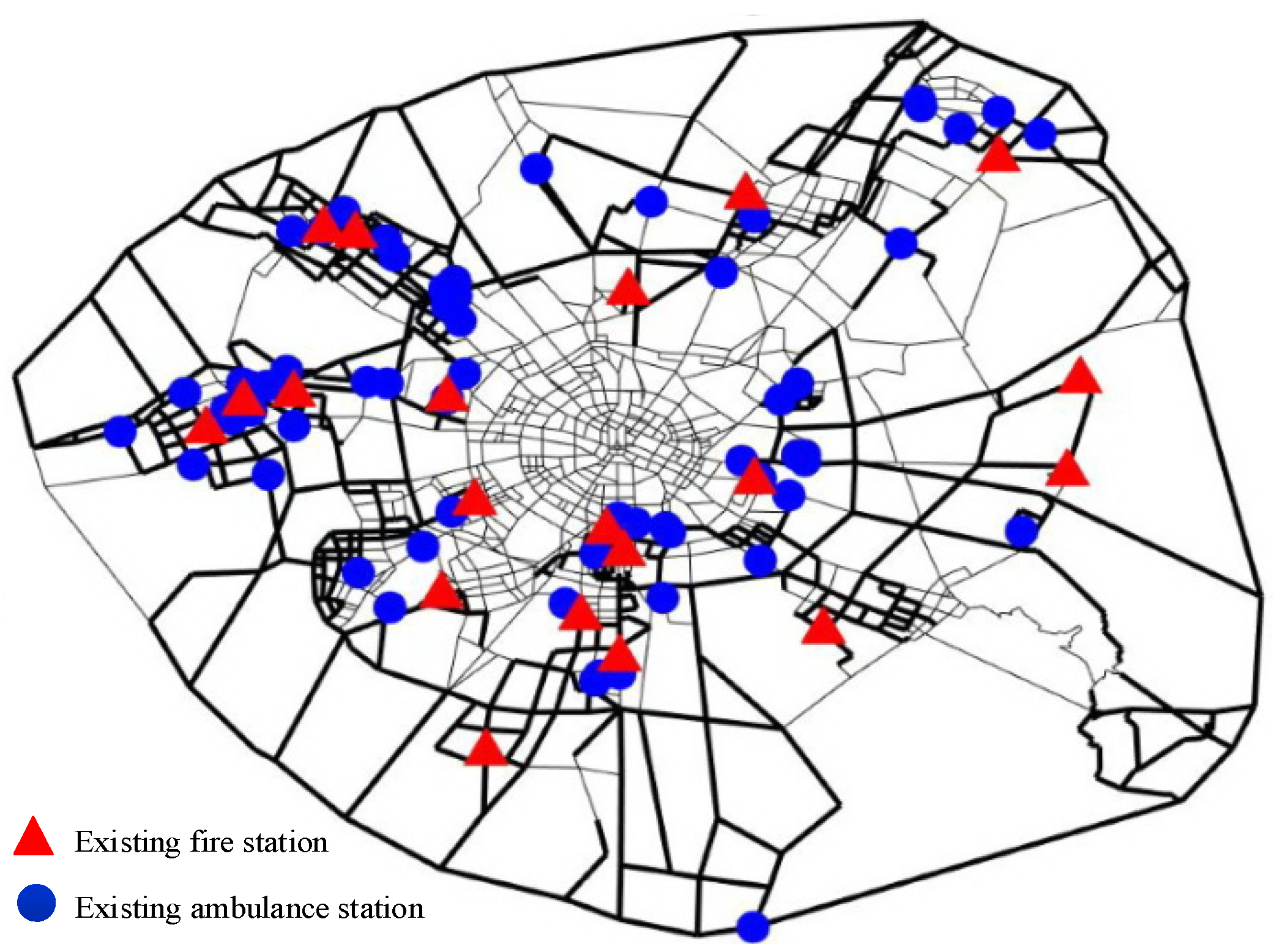
There are 1284 nodes and 2073 edges in the urban road network of Chengdu, which also contains 20 fire stations and 62 ambulance station. There are 326 primary schools. We assume a radius of 800 m around a school defines the “sensitive area” that needs to be avoided by hazmat trucks. In Figure 7a, the green parts constitute these sensitive nodes and edges that cannot be included in the HMTN, which we denote by G^H (V^H, E^H). The red parts in Figure 7b become unconnected due to the removal of the sensitive nodes and edges. After also removing these unconnected parts, the resulting HMTN, with 636 nodes, is depicted in Figure 7c. Figure 8 shows the existing network as well as the HMTN (in thicker lines).

Figure 9 depicts each node in terms of its response and wait times. Since we do not have access to the targets aspired to by the Chengdu City officials, we use their averages as the coverage targets. The average of RTAS is 4.78 min, the corresponding RTFS average is 6.63 min, and the WT average is 3.20 min. Based on these values, currently 302 nodes fall into the poor response area and 40 nodes are in the adequate response area, whereas the response targets are satisfied for the remaining 294 nodes. That means only 46.2% of the city can receive a coordinated and timely response in case of a hazmat transport incident.

7.2. Improving Hazmat Emergency Response in Chengdu

It is not possible to find an optimal solution to this large-scale problem instance with CPLEX within a reasonable time, and hence we apply the proposed genetic algorithm. The parameter setting is shown in Table 6.

We start by focusing on the current situation, where each node is served by the closest emergency and ambulance teams. As mentioned in the previous section, the user preferences can help selecting the best emergency response plan based on one-to-one mapping among the covered nodes and ambulance–fire station pairs. Indeed, it is possible to improve 28 nodes from the adequate response time area to the preferred response time area through a simple reallocation of the resources. Figure 10 shows the response performance, under different user preferences, for the 28 nodes for which coverage was improved. This problem instance is shown in the first column of

Table 7. Solutions with the genetic algorithm.

[NA,NF]	[62,20]		[62,25]	[62,30]	[62,35]	[67,35]	[72,35]	[77,35]	[82,40]	[87,45]
# of New	Ambulance St.	0	0	0	0	5	10	15	20	23
	Fire St.	0	5	10	15	15	15	15	20	24
# of Nodes	Poor → Pref.	0	86	97	107	171	193	203	223	234
	Adeq. → Pref.	28	30	35	37	36	35	36	39	40
Minimum RTAS	Ave. RTAS (min)	4.85	4.84	4.83	4.82	3.92	3.53	3.71	3.13	3.01
	Ave. RTFS (min)	6.64	5.79	5.61	5.55	5.06	4.62	4.85	4.06	4.00
	Ave. WT (min)	3.12	2.38	2.20	2.16	2.03	1.90	1.96	1.72	1.64
Minimum RTFS	Ave. RTAS (min)	4.94	4.94	4.95	4.94	4.03	3.67	3.82	3.30	3.20
	Ave. RTFS (min)	6.63	5.74	5.51	5.37	5.03	4.56	4.81	3.99	3.91
	Ave. WT (min)	3.09	2.37	2.15	2.08	1.98	1.85	1.90	1.68	1.56
Minimum WT	Ave. RTAS (min)	4.94	4.96	5.00	4.97	4.05	3.67	3.87	3.35	3.24
	Ave. RTFS (min)	6.65	5.79	5.62	5.52	5.05	4.58	4.85	4.06	4.05
	Ave. WT (min)	3.03	2.25	2.02	1.92	1.92	1.77	1.73	1.50	1.43

, where NA = 62 and NF = 20, i.e., when no new facilities are built. No nodes in the poor response time area, however, would benefit from such a reallocation of the hazmat incident response resources.

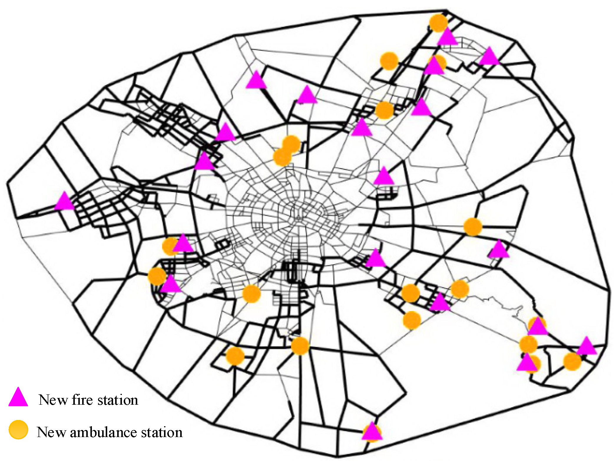
We now focus on another problem instance by setting NA = 82 and NF = 40, which amounts to allowing the construction of up to 20 new ambulance stations and 20 new fire stations. In the second to last column of Table 7, we see that the coverage on a total of 262 nodes can be improved to satisfy the response and wait targets. As a result, 87.4% of the city would enjoy a desirable level of coverage. Note that this amounts to an 89.1% improvement over the current situation. The optimal locations for the new ambulance and fire stations are depicted in Figure 11.

Table 7 also depicts seven additional problem instances to provide the reader with a fuller picture. Arguably, the most interesting case is when [NA, NF] = [87, 45]. Although five new ambulance stations and five new fire stations can be established (compared to [NA, NF] = [82, 40]), the best coverage is obtained by building only three new ambulance stations and four new fire stations. As expected, Table 7 also shows that the average response and wait times are monotonically decreasing as the number of new facilities, and hence the number of nodes in the preferred zone, increase.

We also carried out computational experiments to demonstrate the value of coordination in designing the emergency response system in Chengdu City. To this end, we compared the results of establishing the ambulance and fire stations independently with that of the simultaneous design approach we propose in this paper. The results are depicted in

Table 8. Comparing the solutions with independent and coordinated design.

	Independent Design										Coordinated Design
[NA,NF]	[62,25] + [67,20]		[62,30] + [72,20]		[62,35] + [77,20]		[62,40] + [82,20]		[62,45] + [87,20]		[67,25]	[72,30]	[77,35]	[82,40]	[87,45]
Max # of New
Ambulance St.	0	5	0	10	0	15	0	20	0	25	5	10	15	20	25
Fire St.	5	0	10	0	15	0	20	0	25	0	5	10	15	20	25
# of Nodes
Poor → Pref.	133		153		165		169		169		133	178	203	223	234
Adeq. → Pref.	31		36		40		39		40		33	34	36	39	40
Average WT (min)	2.20		2.01		1.77		1.80		1.80		2.06	1.98	1.73	1.50	1.43

, which is split into two parts: The left side corresponds to the independent design approach, whereas the coordinated design approach results are on the right side. Note that currently [NA, NF] = [62, 20]. In Table 7, the column [62, 25] + [67, 20] represents the construction of five new ambulance stations and five new fire stations by solving the [62, 25] and [67, 20] problems separately, and providing hazmat emergency response with the resulting system. Whereas the [67, 25] column on the right side corresponds to building the same number of stations in a coordinated fashion using the model formulation in Section 4.

It is evident from Table 8 that the coordinated design approach always performs better than the independent design approach, in terms of the resulting wait times. We also observe that the wait time reduction through coordinated design increases substantially with the problem size. In particular, [62, 45] + [87, 20] has a 25.8% longer average wait time than that of [87, 45].

8. Conclusions

This paper has been motivated by the need to design emergency response networks that comprise teams from multiple agencies so that their arrival at the scene of emergency is well-coordinated. Focusing on the problem with two response resources, we can define the poor, adequate, and preferred responses in terms of the target response and wait times. This enables us to expand the maximal covering problem formulation to incorporate two resources, where the objective is to maximize the number of possible emergency sites with the preferred response. The conceptual framework is generalizable to more than two resources, although the number of response types would be combinatorial and, hence, the arising mathematical models would be cumbersome.

From the perspective of policymakers and emergency planners, our findings suggest that significant improvements could be achieved by deploying a systems view in planning emergency response networks. Typically, these systems are expanded gradually, i.e., the decisions to add one (or more) ambulance or fire station(s) are made sequentially, as budgets become available. This paper clearly highlights the need to have a long-term perspective for expanding the existing networks, rather than adopting a myopic approach by focusing on the best sites for only the new stations to be established in the short term. Our work also points out the need for streamlining the network development process for the specialty teams that need to collaborate, although their organizational structure can be separate, e.g., ambulance services and fire services. A collaborative development of such separately managed systems would certainly pay off in terms of the joint response time to the incidents.

This paper is at the strategic level, focusing on the structure of emergency response systems to maximize the coordination among multiple specialty teams. At the tactical level, these systems have benefited significantly from artificial intelligence (AI)-based enhancements. Ref. [33] is a recent systematic review of the literature on AI-based emergency response systems. Among several enhancements, the authors highlighted that AI has significantly improved emergency vehicle routing and congestion management by enabling real-time traffic analysis, dynamic route optimization, and predictive analytics. The AI-based enhancements in real-time decision making and communication for emergency response are also discussed in [34].

Our work is a first step in the development of an analytical framework for the coordination of the multiple resources involved in emergency response. It has several limitations, however, that need to be resolved in future work to improve its performance in practical settings. For example, we do not consider traffic congestion and the resulting uncertainties in our modeling framework. This is a realistic assumption since all emergency vehicles enjoy priority lanes and/or courtesy from the other drivers to minimize the impact of traffic. In metropolitan cities, however, the traffic congestion is so high that it can affect even the emergency vehicles. In such cases, explicit incorporation of the impact of traffic congestion on emergency vehicle travel times would increase the realism of our planning model. Another direction would be the expansion of the modeling framework to capture the hierarchical nature of the response resources to be deployed, such as the national response networks in the U.S. and Canada.

References

- US DoT. Glossary: Simplified Guide to the Incident Command System for Transportation Professionals. 2018. Available online: https://ops.fhwa.dot.gov/publications/ics_guide/glossary.htm (accessed on 20 March 2025).
- Public Safety Canada. Emergency Management. 2018. Available online: https://www.publicsafety.gc.ca/cnt/mrgnc-mngmnt/index-en.aspx (accessed on 19 March 2025).
- Ministry of Community Safety and Correctional Services. Fire Marshall’s Communiqué 2016-05. 2016. To Get a Copy of This Communiqué, Send an Email to AskOFM@ontario.ca. Available online: https://www.ontario.ca/page/office-fire-marshals-communiques-and-bulletins#2016communiques (accessed on 20 March 2025).
- Church, R.; ReVelle, C. The maximal covering location problem. Pap. Reg. Sci. 1974, 32, 101–118. [Google Scholar] [CrossRef]
- Li, X.; Zhao, Z.; Zhu, X.; Wyatt, T. Covering models and optimization techniques for emergency response facility location and planning: A review. Math. Methods Oper. Res. 2011, 74, 281–310. [Google Scholar] [CrossRef]
- Daskin, M.S. Application of an expected covering model to emergency medical service system design. Decis. Sci. 1982, 13, 416–439. [Google Scholar]
- Hogan, K.; Revelle, C. Concepts and Applications of Backup Coverage. Manag. Sci. 1986, 32, 1434–1444. [Google Scholar]
- Gendreau, M.; Laporte, G.; Semet, F. Solving an ambulance location model by tabu search. Locat. Sci. 1997, 5, 75–88. [Google Scholar] [CrossRef]
- Marianov, V.; Serra, D. Probabilistic, Maximal Covering Location—Allocation Models for Congested Systems. J. Reg. Sci. 1998, 38, 401–424. [Google Scholar]
- Gandhi, R.; Khuller, S.; Srinivasan, A. Approximation Algorithms for Partial Covering Problems. J. Algorithms 2001, 53, 55–84. [Google Scholar]
- Brotcorne, L.; Laporte, G.; Semet, F. Ambulance location and relocation models. Eur. J. Oper. Res. 2003, 147, 451–463. [Google Scholar] [CrossRef]
- Berman, O.; Krass, D.; Drezner, Z. The gradual covering decay location problem on a network. Eur. J. Oper. Res. 2003, 151, 474–480. [Google Scholar] [CrossRef]
- Galvão, R.D.; Chiyoshi, F.Y.; Morabito, R. Towards unified formulations and extensions of two classical probabilistic location models. Comput. Oper. Res. 2005, 32, 15–33. [Google Scholar] [CrossRef]
- Jia, H.; Ordóñez, F.; Dessouky, M.M. Solution approaches for facility location of medical supplies for large-scale emergencies. Comput. Ind. Eng. 2007, 52, 257–276. [Google Scholar] [CrossRef]
- Sorensen, P.; Church, R. Integrating expected coverage and local reliability for emergency medical services location problems. Socio-Econ. Plan. Sci. 2010, 44, 8–18. [Google Scholar] [CrossRef]
- Salman, F.S.; Yücel, E. Emergency facility location under random network damage: Insights from the Istanbul case. Comput. Oper. Res. 2015, 62, 266–281. [Google Scholar] [CrossRef]
- Paul, N.R.; Lunday, B.J.; Nurre, S.G. A multiobjective, maximal conditional covering location problem applied to the relocation of hierarchical emergency response facilities. Omega 2017, 66, 147–158. [Google Scholar] [CrossRef]
- Berman, O.; Hajizadeh, I.; Krass, D.; Rahimi-Vahed, A. Reconfiguring a set of coverage-providing facilities under travel time uncertainty. Socio-Econ. Plan. Sci. 2018, 62, 1–12. [Google Scholar] [CrossRef]
- Liu, Y.; Fan, Z.-P.; Yuan, Y.; Li, H. A FTA-based method for risk decision-making in emergency response. Comput. Oper. Res. 2014, 42, 49–57. [Google Scholar] [CrossRef]
- Verma, A.; Gaukler, G.M. Pre-positioning disaster response facilities at safe locations: An evaluation of deterministic and stochastic modeling approaches. Comput. Oper. Res. 2014, 62, 197–209. [Google Scholar] [CrossRef]
- Abdelgawad, H.; Abdulhai, B. Emergency evacuation planning as a network design problem: A critical review. Transp. Lett. 2009, 1, 41–58. [Google Scholar] [CrossRef]
- Murray-Tuite, P.; Wolshon, B. Evacuation transportation modeling: An overview of research, development, and practice. Transp. Res. Part C 2013, 27, 25–45. [Google Scholar] [CrossRef]
- Santos, G.; Aguirre, B.E. A Critical Review of Emergency Evacuation Simulation Models. In Proceedings of the Building Occupant Movement During Fire Emergencies, Gaithersburg, MD, USA, 10–11 June 2004. [Google Scholar]
- Saccomanno, F.F.; Allen, B. Locating emergency response capability for dangerous goods incidents on a road network. Transp. Hazard. Mater. 1988, 1, 1–9. [Google Scholar]
- Erkut, E.; Tjandra, S.A.; Verter, V. Chapter 9 Hazardous Materials Transportation. In Handbooks in Operations Research and Management Science; Barnhart, C., Laporte, G., Eds.; Elsevier: Amsterdam, The Netherlands, 2007; pp. 539–621. [Google Scholar] [CrossRef]
- Berman, O.; Verter, V.; Kara, B.Y. Designing emergency response networks for hazardous materials transportation. Comput. Oper. Res. 2007, 34, 1374–1388. [Google Scholar] [CrossRef]
- Zografos, K.G.; Androutsopoulos, K.N. A decision support system for integrated hazardous materials routing and emergency response decisions. Transp. Res. Part C Emerg. Technol. 2008, 16, 684–703. [Google Scholar] [CrossRef]
- Taslimi, M.; Batta, R.; Kwon, C. A Comprehensive Modeling Framework for Hazmat Network Design, Hazmat Response Team Location, and Equity of Risk. Comput. Oper. Res. 2017, 79, 119–130. [Google Scholar] [CrossRef]
- Zhao, J.; Ke, G.Y. Optimizing Emergency Logistics for the Offsite Hazardous Waste Management. J. Syst. Sci. Syst. Eng. 2019, 28, 747–765. [Google Scholar] [CrossRef]
- Mohabbati-Kalejahi, N.; Vinel, A. Robust Hazardous Materials Closed-Loop Supply Chain Network Design with Emergency Response Teams Location. Transp. Res. Rec. 2021, 2675, 306–329. [Google Scholar] [CrossRef]
- Ke, G.Y. Managing reliable emergency logistics for hazardous materials: A two-stage robust optimization approach. Comput. Oper. Res. 2022, 138, 105557. [Google Scholar] [CrossRef]
- Wang, Y.; Wang, J.; Chen, J.; Liu, K. Optimal Location of Emergency Facility Sites for Railway Dangerous Goods Transportation under Uncertain Conditions. Appl. Sci. 2023, 13, 6608. [Google Scholar] [CrossRef]
- Bajwa, A. AI-based emergency response systems: A systematic literature review on smart infrastructure safety. Am. J. Adv. Technol. Eng. Solut. 2025, 1, 174–200. [Google Scholar] [CrossRef]
- Li, Z. Leveraging AI automated emergency response with natural language processing: Enhancing real-time decision making and communication. Appl. Comput. Eng. 2024, 71, 1–6. [Google Scholar] [CrossRef]
Disclaimer/Publisher’s Note: The statements, opinions and data contained in all publications are solely those of the individual author(s) and contributor(s) and not of MDPI and/or the editor(s). MDPI and/or the editor(s) disclaim responsibility for any injury to people or property resulting from any ideas, methods, instructions or products referred to in the content. |
© 2025 by the authors. Licensee MDPI, Basel, Switzerland. This article is an open access article distributed under the terms and conditions of the Creative Commons Attribution (CC BY) license (https://creativecommons.org/licenses/by/4.0/).