Abstract
Elastic wavefield separation in anisotropic media is essential for seismic imaging but remains challenging due to complex interactions among multiple wave modes. Traditional methods often rely on solving the Christoffel equation, which is computationally expensive, particularly in heterogeneous models. This study proposes a deep learning-based approach using a cross-attention U-Net architecture to achieve efficient vector decomposition of elastic wavefields. The model employs a dual-branch encoder with cross-attention mechanisms to preserve and exploit inter-component relationships among wavefield components. The network was trained on patches extracted from the BP (British Petroleum) 2007 anisotropic benchmark model, with ground truth labels being generated via low-rank approximation methods. Quantitative evaluations show that the cross-attention U-Net outperforms a baseline U-Net, improving the peak signal-to-noise ratio(PSNR) by 1.25 dB (44.10 dB vs. 42.85 dB) and structural similarity index (SSIM) by 0.014 (0.904 vs. 0.890). The model demonstrates effective generalization to larger domains and different geological settings, validated on both the extended BP model and the Hess vertically transversely isotropic (VTI) model. Overall, this approach provides a computationally efficient alternative to traditional separation methods while maintaining physical consistency in the separated wavefields.
1. Introduction
Elastic wavefields contain multiple wave modes, including compressional (P), shear (S), and converted waves, which naturally combine during propagation. This combination creates challenges in seismic imaging and inversion, especially in elastic reverse-time migration (RTM), where interactions between wave modes can produce unwanted artifacts. To enhance the image quality, separating these wave modes and processing them independently before applying imaging conditions can be helpful [1,2].
Wave mode separation and vector decomposition are two main methods that are used to separate elastic wavefields. Wave mode separation uses differences in polarization properties to distinguish P- and S-waves. In isotropic media, P-waves have no curl, and S-waves have no divergence, allowing for separation through the Helmholtz decomposition method, which uses divergence and curl operators [3,4]. In anisotropic media, the polarizations of quasi-P (qP) and quasi-S (qS) waves differ from their wave vectors due to directional dependencies in elastic properties, requiring more complex approaches beyond simple divergence and curl operations. Vector decomposition, introduced by Zhang and McMechan (2010) [5], takes a different approach by projecting wavefields onto polarization vectors that are calculated from the Christoffel equation in the wavenumber domain. While this method preserves the amplitude, phase, and vector characteristics of the separated waves, it shares a common challenge with wave mode separation methods: both approaches require solving the Christoffel equation, which is computationally demanding and needs to be repeated for each spatial location and propagation direction, creating challenges for large-scale or heterogeneous models.
To address the computational limitations of solving the Christoffel equation, several advancements have been proposed. Yan and Sava (2009) [1] introduced nonstationary spatial filters that adapt to local anisotropic properties. These filters still use polarization vectors from the Christoffel equation but represent them as localized filtering operators in the space domain, reducing the computational overhead while maintaining separation accuracy. Building on this, Yan and Sava (2011) [6] developed a mixed-domain algorithm that integrates space and wavenumber domain operations. By approximating the medium’s heterogeneity with reference models, this approach reduces the calculations that are needed for polarization vectors. Cheng and Fomel (2014) [2] proposed using Fourier integral operators with low-rank approximations for both wave mode separation and vector decomposition methods. This modification enables more efficient wavefield separation without directly solving the Christoffel equation at every spatial point, making these methods more practical for large, heterogeneous models. Zhou and Wang (2016) [7] developed an approach that simplifies the separation operators to forms resembling divergence and curl operators in isotropic media. Their method uses rotated wave vectors and Poynting vectors to approximate polarization directions, reducing the computational complexity in complex geological settings. Further research has extended these methods to low-symmetry anisotropic media. Sripanich et al. (2017) [8] adapted vector decomposition for orthorhombic, monoclinic, and triclinic models, addressing challenges like polarization discontinuities and singularities through smoothing filters and local signal–noise orthogonalization. These improvements enhance the computational efficiency and broaden the application of elastic wavefield separation methods to more complex geological models.
Recent deep learning (DL) advances have provided useful tools for seismic wavefield processing, addressing challenges in wave mode separation and vector decomposition. U-Net-based convolutional neural networks (CNNs) have emerged as a common approach. Huang et al. (2021) [9] developed a U-Net model to separate qP and qS wavefields in anisotropic media. By incorporating techniques such as dilated convolutions and anti-aliasing, the model effectively handled complex anisotropic wavefields while maintaining the spatial resolution. Sun et al. (2023) [10] introduced a U-ConvNeXt architecture that integrates ConvNeXt blocks—known for their enhanced feature extraction and representation capabilities—into a U-Net framework. This architecture enabled cleaner separation of P- and S-wave components, reduced artifacts, and showed computational efficiency suitable for large-scale seismic data analysis. Generative Adversarial Networks (GANs) have also been applied to wave mode separation. Kaur et al. (2021) [11] proposed a Cycle-GAN framework to decouple qP and qS wavefields in anisotropic media. This method eliminated the need for solving the computationally intensive Christoffel equation and achieved reliable separation of wave modes in highly anisotropic environments.
While previous deep learning methods [9,10,11] have shown promise in wavefield decomposition, they do not incorporate mechanisms to explicitly capture the interactions between P- and S-wave components. To address this limitation, this study proposes a U-Net-based architecture enhanced with cross-attention mechanisms for elastic wavefield vector decomposition in anisotropic media. The model employs a dual-branch encoder to process horizontal and vertical displacement components separately, while the cross-attention enables dynamic feature exchange between them. This structure allows the network to preserve the physical characteristics of each wave mode and to focus on the most relevant features across components, thereby improving the decomposition accuracy and efficiency. The cross-attention mechanism is particularly effective in capturing the complex inter-mode relationships that are inherent to anisotropic wavefields.
2. Theoretical Framework
2.1. Elastic Wave Vector Decomposition in Anisotropic Media
Wave mode separation in elastic wavefields is commonly performed using Helmholtz decomposition, which allows the vector wavefield U = (Ux, Uy, Uz) to be expressed as the sum of P- and S-wave components:
The P-wave component satisfies ∇ × UP = 0, while the S-wave component satisfies ∇ ⋅ US = 0 [3]. However, in anisotropic media, the polarization directions of qP and qS waves are not necessarily aligned with the wave vector k, rendering simple divergence and curl operators insufficient for mode separation [4]. Instead, the vector wavefield must be projected onto the polarization vectors of each wave mode [2,5].
The polarization vectors pqP, pqSV, and pqSH are computed by solving the Christoffel equation:
where C is the stiffness tensor, ρ is the mass density, V is the phase velocity of each wave mode, and p is the polarization vector. To obtain a wave vector decomposition that is analogous to Helmholtz decomposition, the vector wavefield is first expressed in the wavenumber domain. Applying the Fourier transform to the vector wavefield U results in its representation in the wavenumber domain as . The P- and S-wave separation expressions in isotropic media can be reformulated as follows:
Since the wave vector k does not necessarily align with the polarization directions in anisotropic media, it is replaced with the polarization vectors obtained from the Christoffel equation, yielding the anisotropic wave vector decomposition:
This formulation extends Helmholtz decomposition to anisotropic media by incorporating polarization vectors derived from the Christoffel equation, ensuring physically accurate separation of elastic wave modes.
2.2. Low-Rank Approximation for Wave Vector Decomposition
Wave vector decomposition, as demonstrated in Section 2.1, projects the vector wavefield onto the polarization vectors obtained from the Christoffel equation [5]. However, the direct implementation of these projections requires solving the Christoffel equation at every spatial location and propagation direction, leading to high computational costs. This complexity arises because polarization vectors are spatially dependent and must be computed individually for each grid point in a heterogeneous anisotropic medium.
Applying the inverse Fourier transform to Equation (4), the wavefield decomposition in the space domain is expressed as follows:
where pqP(x, k), pqSV(x, k), and pqSH(x, k) represent the polarization vectors for the qP, qSV, and qSH waves at position x and wavenumber k, respectively. Each separated wavefield UqsP, α is computed by summing up the spatial indices β ∈ {x, y, z}, where pqP,α(x, k) denotes the α-th component of the polarization vector. This formulation allows the wave mode separation to be expressed as nonstationary filtering, but the computational cost remains high due to the need for grid-by-grid polarization vector computation.
To further improve the computational efficiency, the wave mode decomposition operator can be reformulated using matrix notation as follows [2]:
where B(x, km) and C(xn, k) are mixed-domain matrices that capture variations in wavefield properties, Amn is a low-rank matrix that approximates the decomposition operator, Nx is the total number of spatial grid points in the computational domain, and N is the numerical rank used in the low-rank decomposition.
Since M, N ≪ Nx, this decomposition significantly reduces the computational cost. The direct computation of wave mode decomposition has a complexity of O() due to the need for solving the Christoffel equation at every spatial location. However, low-rank decomposition reduces the complexity to O(). This decomposition is implemented using pivoted QR (orthogonal-triangular) decomposition, enabling the precomputation of mode separation operators in a compact form. While low-rank approximation improves efficiency, the rank N controls the balance between accuracy and cost. A higher rank provides greater accuracy but increases computational demands, whereas a lower rank accelerates calculations at the expense of some accuracy loss. To avoid the extensive computational cost of solving the Christoffel equation across large datasets, low-rank approximation was used to generate ground truth labels for training the deep learning model applied in this study.
2.3. Cross-Attention for Vector Decomposition
In vector decomposition, seismic wavefields consist of multiple displacement components, each containing contributions from different wave modes. Traditional deep learning models for wave mode separation typically concatenate these components into a single input, allowing the network to process them jointly. However, in vector decomposition, each displacement component contains distinct qP and qS wave contributions. Treating all components as a single input may limit the model’s ability to effectively disentangle these mixed wave modes.
A more structured approach is to encode each displacement component separately, ensuring that the model learns distinct features for each mode. While this enhances feature extraction within individual components, it introduces a drawback: the absence of direct interaction between components during encoding. Since displacement components share underlying physical relationships, ignoring these interdependencies could reduce the model’s ability to accurately decompose the wavefield.
To address this limitation, cross-attention enables dynamic feature exchange between separately encoded components. Unlike self-attention, which captures dependencies within a single input sequence, cross-attention establishes relationships across distinct inputs [12,13]. This mechanism allows each displacement component to selectively focus on relevant features from others, facilitating improved wave mode separation. Cross-attention is computed by exchanging information between different displacement components. This process is bidirectional, ensuring that each component benefits from interactions with the others. The general form of cross-attention is expressed as follows:
where D = 3 represents the number of spatial components (x, y, z), and i, j ∈ {x, y, z} ensure that each component attends to the others. Here, Qi is the query representation obtained from the feature embeddings of displacement component i, while Kj and Vj correspond to the key and value embeddings of component j. The scaling factor dk normalizes the attention scores to stabilize training. This formulation ensures that each displacement component retains its physical consistency while incorporating inter-component dependencies that would otherwise be lost when processing components independently.
By integrating cross-attention, the model enhances its ability to maintain physical consistency across decomposed wave modes. This is particularly relevant in anisotropic media, where wave mode interactions vary due to differences in elastic properties. Furthermore, cross-attention has been widely used in multi-modal learning, where multiple input modalities must interact to enhance the feature extraction [13,14]. In seismic data processing, displacement components serve as distinct yet correlated feature spaces. When processed independently, they may lose valuable interactions, which cross-attention compensates for by selectively integrating relevant information across components.
2.4. Network Architecture
The proposed model is based on a U-Net architecture [15], enhanced with cross-attention mechanisms to improve vector decomposition while preserving inter-component relationships. Unlike conventional approaches that concatenate displacement components into a single input, this model processes them separately in the encoder and integrates cross-attention in the decoder to facilitate feature exchange. This structure ensures that the vector decomposition remains physically meaningful while improving the separation process.
The model takes a seismic wavefield snapshot as input, where the horizontal and vertical displacement components, ux and uz, serve as the input channels. Each displacement component contains contributions from both qP and qS waves, which must be properly separated to ensure accurate vector decomposition. Since this study focuses on 2D wavefield decomposition, the analysis is restricted to qP and qS waves, without considering separate shear wave polarizations such as qSH and qSV. The network is designed to output two channels, ux_qS and uz_qS, corresponding to the qS wave components of the horizontal and vertical displacements. The qP components, ux_qP and uz_qP, are then inferred using the physical constraint:
Empirical results indicate that learning S-wave components directly and computing P-wave components as residuals leads to improved separation performance, making this a preferred approach for training.
As illustrated in Figure 1, the network consists of three main components: an encoder, a cross-attention module, and a decoder. The encoder follows a dual-branch structure, where the two displacement components are processed independently through separate encoding paths. Each encoding path consists of multiple down-sampling stages, applying residual blocks [16] for feature extraction while progressively reducing the spatial resolution through pooling layers. This design allows the network to learn independent representations for each component while preserving their structural integrity. Unlike conventional U-Net models, which process displacement components jointly, this approach ensures that the unique polarization characteristics in ux and uz are retained during feature extraction.
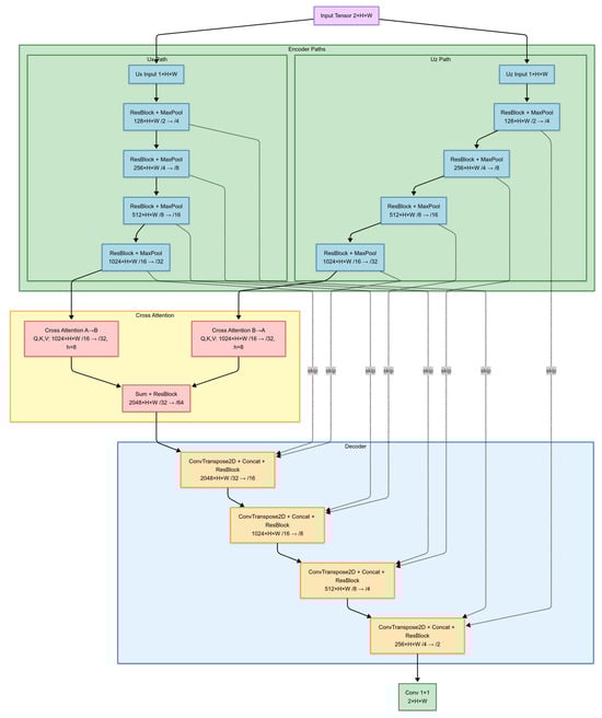
Figure 1.
Architecture of the proposed cross-attention-based U-Net model for seismic wavefield decomposition. The network consists of three main components: an encoder, a cross-attention module, and a decoder. The encoder follows a dual-path structure, where horizontal (ux) and vertical (uz) displacement components are processed separately through independent encoding paths. The cross-attention modules facilitate feature exchange between the two paths, ensuring improved vector decomposition while preserving inter-component relationships. The decoder reconstructs the qS wave components (ux_qS, uz_qS), while the qP wave components (ux_qP, uz_qP) are inferred using a physical constraint.
To facilitate feature exchange between the encoded displacement components, cross-attention is introduced before the decoder. Instead of simply concatenating feature maps before decoding, cross-attention selectively integrates relevant information from one component into the other, ensuring that the decomposition process remains consistent with the underlying physical relationships between wave modes. The cross-attention mechanism enables dynamic feature interaction and reinforces inter-component dependencies, which are essential for robust wave mode separation, particularly in anisotropic media. Following cross-attention, the decoder mirrors the hierarchical structure of the encoders. For each up-sampling step, transposed convolutions restore spatial resolution, and feature maps from the corresponding encoder layers are concatenated through skip connections to retain fine-scale structural details [15]. This ensures that high-resolution, near-surface information—preserved in the encoder’s earlier stages—remains accessible during wave mode separation.
2.5. Training
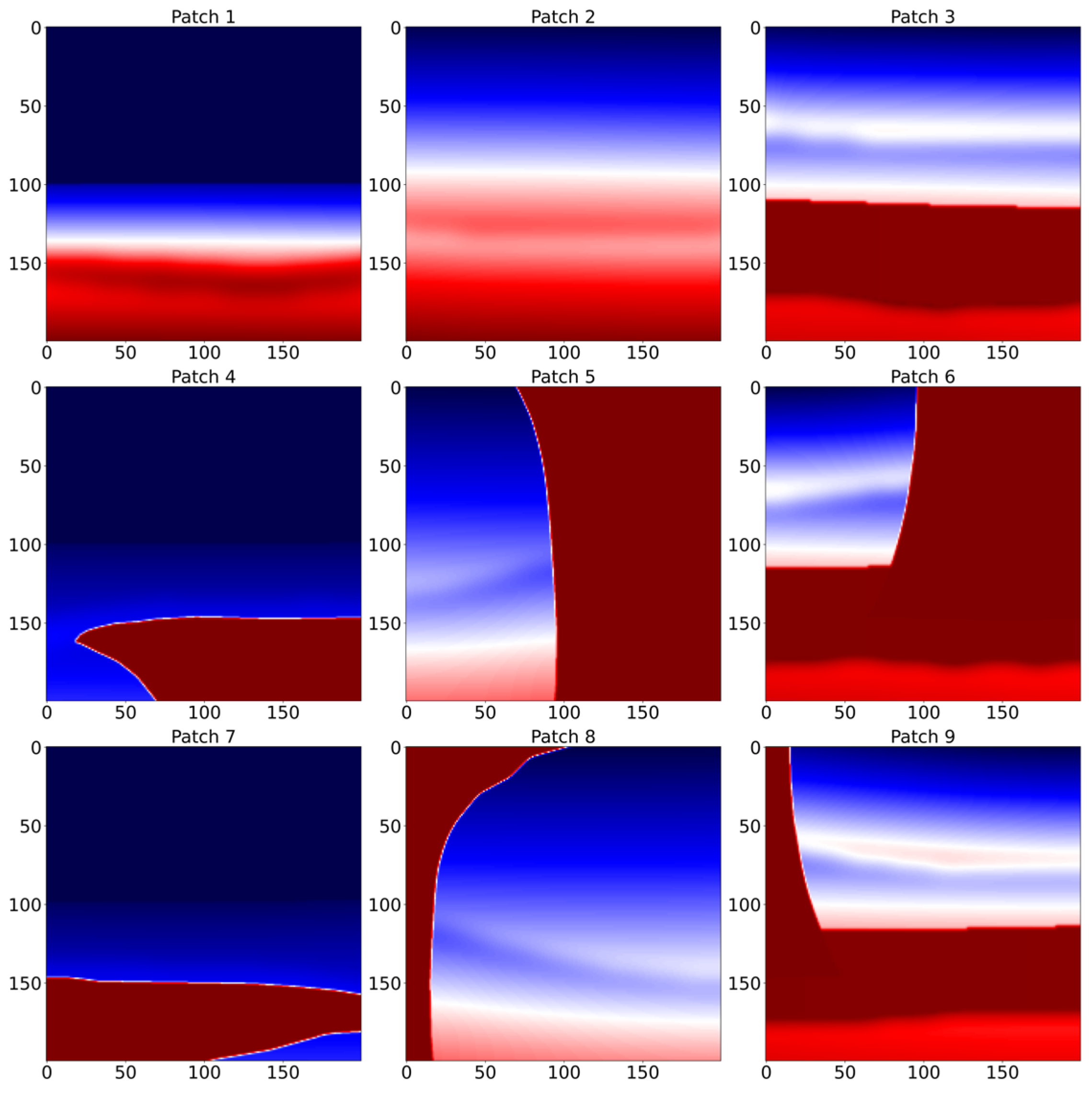
To evaluate the effectiveness of the proposed cross-attention-based wavefield decomposition, a modified version of the BP 2007 anisotropic benchmark model, a widely used anisotropic subsurface model, was employed. Figure 2 shows the elastic properties of the medium: P-wave velocity (Vp), S-wave velocity (Vs), and Thomsen parameters (ϵ, δ). For training, the model domain was partitioned into 200 × 200 subregions, yielding 60 distinct patches. To increase variability and improve generalization, 30 additional patches were generated using standard data augmentation techniques, including random flips and minor scaling. The patch size (200 × 200) and the number of augmented samples (30) were empirically chosen to balance model performance and computational cost. These parameters were fixed during training for consistency but may be adjusted in future studies depending on the application. The process of extracting patches from the full model is illustrated in Figure 3, which provides an example of how the domain is segmented for training.
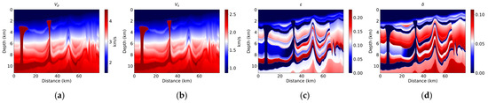
Figure 2.
Elastic properties of the modified BP 2007 anisotropic benchmark model. (a) P-wave velocity (Vp), (b) S-wave velocity (Vs), (c) Thomsen parameter ϵ, and (d) Thomsen parameter δ. These properties define the subsurface anisotropic characteristics used for wavefield decomposition.
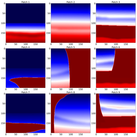
Figure 3.
Example of the patch extraction process from the modified BP 2007 anisotropic benchmark model. The full model domain is divided into 200 × 200 subregions, yielding 60 distinct patches for training. Additionally, 30 augmented patches are generated using random flipping and minor scaling. Red and blue denote high and low values of the physical property, respectively.
For each patch, wave propagation is simulated under five different source locations, ensuring that the network is exposed to wavefields from multiple illumination angles. From each source simulation, 5 temporal snapshots of the propagating wavefield are extracted, leading to a total of 25 wavefield snapshots per patch. The snapshots are randomly selected from a time window excluding the initial 0.2 s of simulation, with at least 0.15 s between each selection to ensure sufficient temporal diversity. The ground truth labels are generated via the low-rank approximation method described in Section 2.2, allowing us to bypass explicit Christoffel equation solvers during training.
During training, two U-Net variants are compared—one with multi-head cross-attention integrated at the deepest encoder level and one without. Both variants utilize residual blocks in the encoder and decoder to facilitate gradient flow. The dataset is randomly partitioned into training, validation, and testing splits, with 64% of the data used for training, 16% for validation, and 20% for testing. All network weights are initialized by the Kaiming normal scheme [17] to stabilize the early training. Optimization is performed using the Adam optimizer [18], with an initial learning rate of 1.5 × 10⁻⁴. Training typically proceeds for up to 200 epochs with a patience-based early-stopping criterion set to 30 epochs. To further regularize the model, a minor physics-informed penalty (coefficient 0.01) is included within the loss function to encourage physically consistent separation. This term is particularly useful in noisy or highly heterogeneous scenarios, where purely data-driven separation may overfit spurious features.
The training was conducted using an NVIDIA RTX 4090 Graphics Processing Unit (GPU; NVIDIA Corporation, Santa Clara, CA, USA) with CUDA (Compute Unified Device Architecture) acceleration. For the baseline U-Net model (without cross-attention), the total training time was approximately 4925 s, while the cross-attention U-Net required approximately 6487 s. This increase in training time reflects the additional computational complexity that is introduced by the attention mechanism.
3. Results
3.1. Comparative Evaluation of the U-Net and Cross-Attention U-Net
Table 1 compares the overall performance of the baseline U-Net model and the proposed cross-attention U-Net on the test set. The evaluated metrics include the peak signal-to-noise ratio (PSNR), structural similarity index measure (SSIM), and channel-wise SSIM values for each separated component (ux_qp, ux_qs, uz_qp, uz_qs). Higher PSNR and SSIM scores indicate better decompositions of qP and qS energy from the original displacement fields.

Table 1.
Comparison of the baseline U-Net and the cross-attention U-Net in terms of peak signal-to-noise ratio (PSNR), structural similarity index measure (SSIM), and channel-wise SSIM (ux_qp, ux_qs, uz_qp, uz_qs). Higher PSNR and SSIM values indicate better overall decomposition performance.
Across all quantitative metrics, the cross-attention U-Net achieves lower reconstruction errors and higher fidelity compared to the U-Net. The mean PSNR and SSIM values, for instance, increase from 42.8360 dB to 44.1008 dB and from 0.8897 to 0.9043, respectively, indicating that incorporating cross-attention enables the network to better capture the relationships between the horizontal and vertical displacement fields. The channel-wise SSIM values also improve consistently, suggesting that each separated wave mode (ux_qp, ux_qs, uz_qp, uz_qs) benefits from the mutual exchange of complementary features across different displacement components.
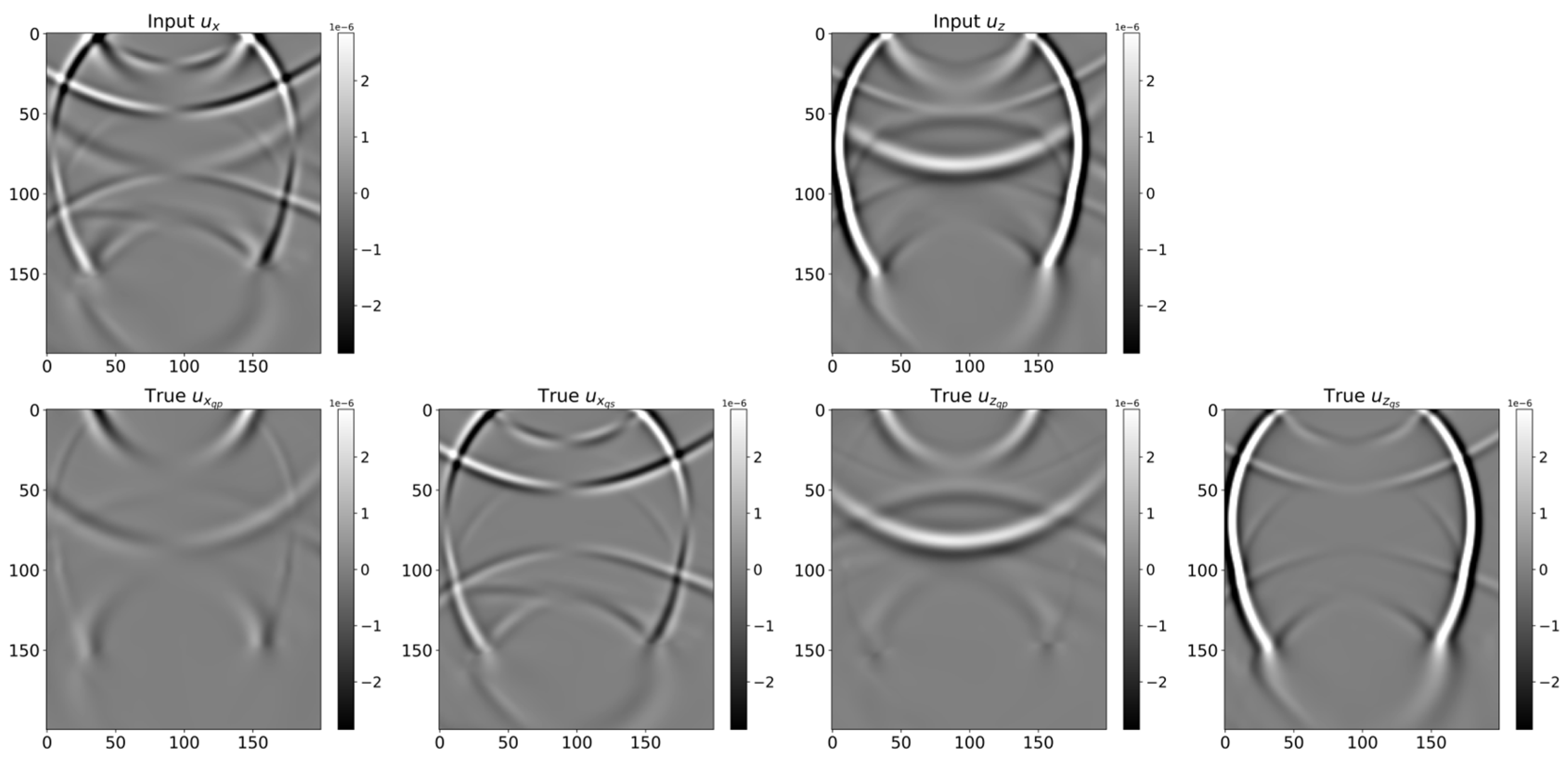
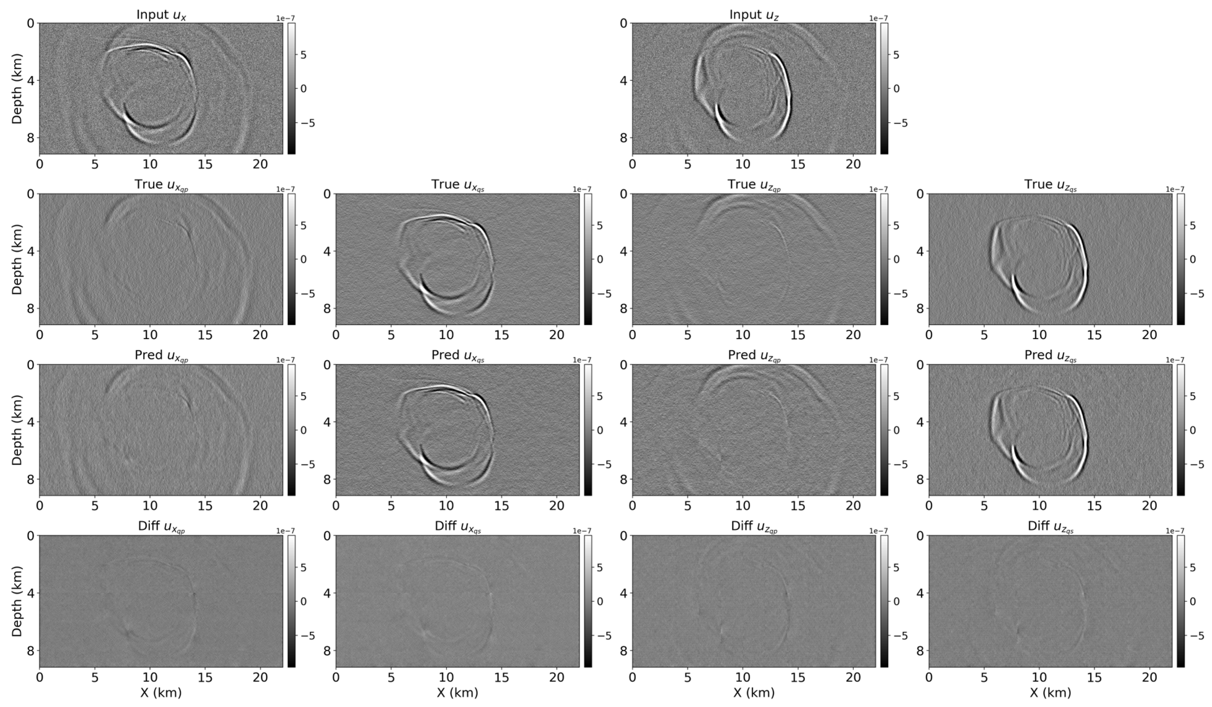
Figure 4 shows an example input wavefield (ux and uz; first row), along with the corresponding ground truth snapshots (ux_qp, ux_qs, uz_qp, uz_qs) in the second row. These ground truth snapshots were generated using the low-rank approximation method (Section 2.2) to ensure a physically consistent reference for vector decomposition.
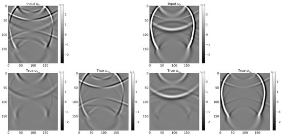
Figure 4.
Example of an input snapshot (top row: ux and uz) and the corresponding ground truth qP and qS components (bottom row: ux_qp, ux_qs, uz_qp, uz_qs). Ground truth labels are generated via the low-rank approximation method.
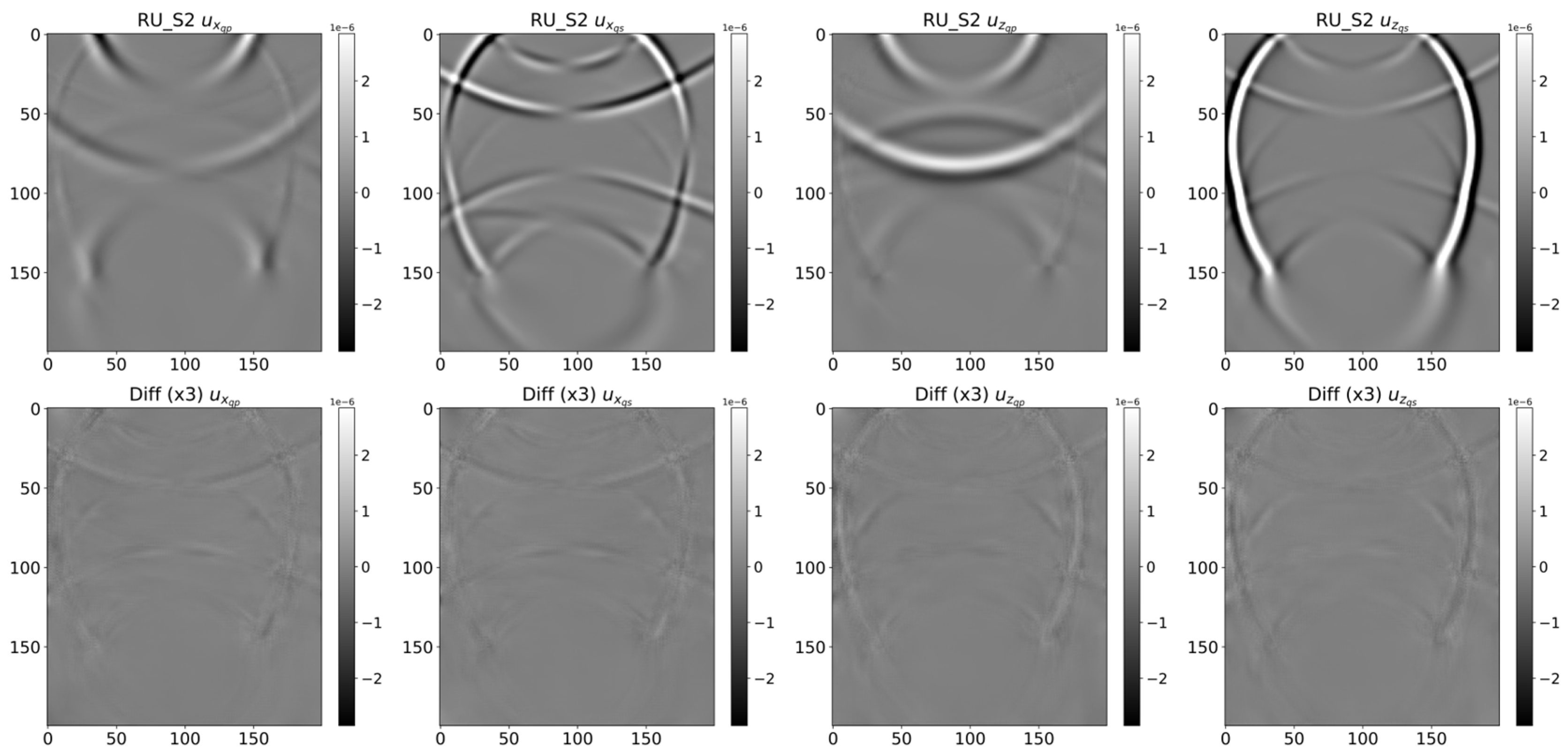
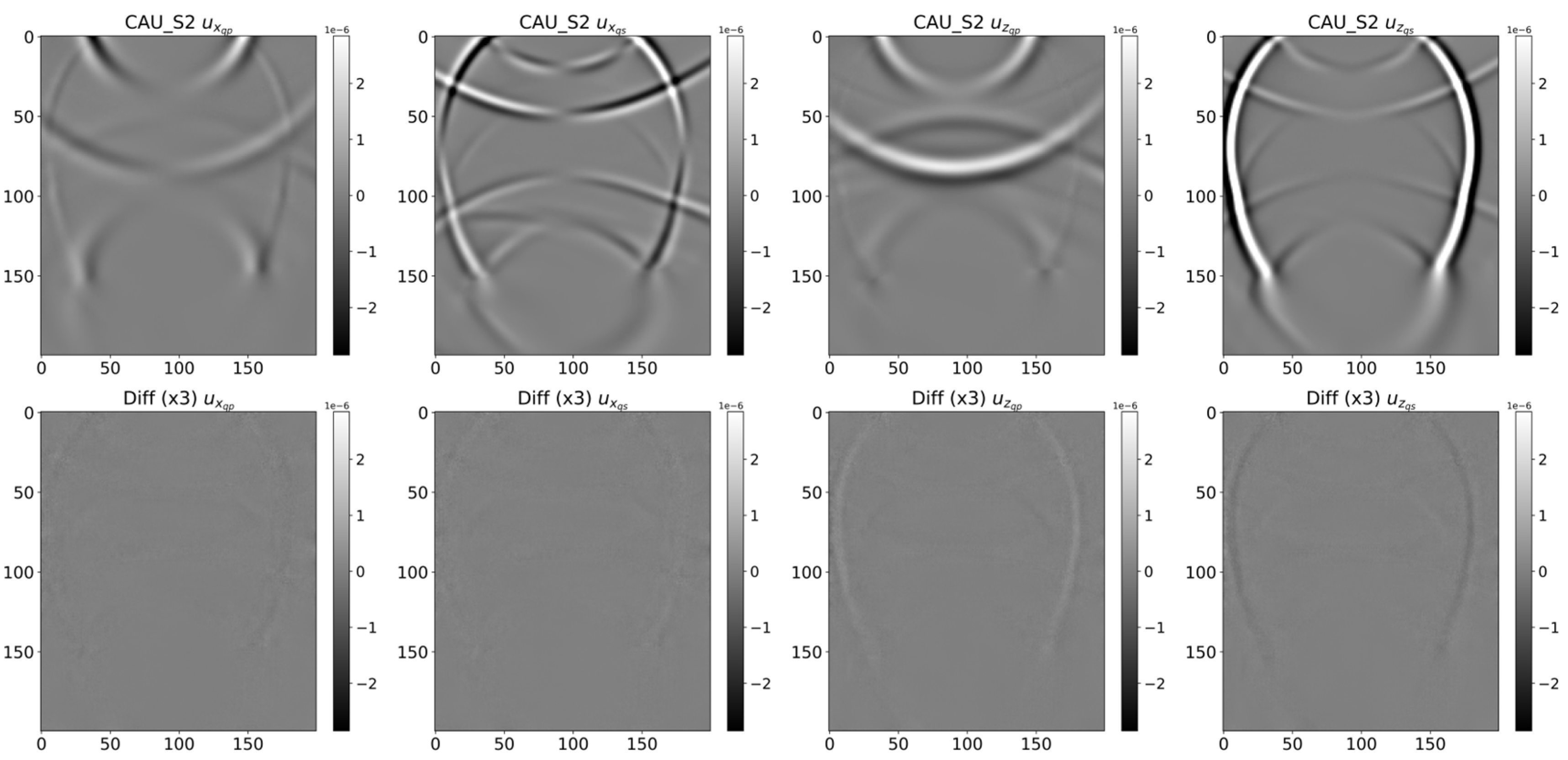
Figure 5 and Figure 6 compare the results of the U-Net and the cross-attention U-Net for the same snapshot. In each figure, the top row shows the predicted components, and the bottom row displays the difference from the ground truth. These difference (residual) plots are scaled by a factor of three (×3) to enhance the visibility of local errors and artifacts. In Figure 5, the U-Net successfully separates most of the P- and S-wave energy but leaves some pronounced artifacts near complex geological boundaries and areas of strong reflection. In contrast, Figure 6 demonstrates that the cross-attention U-Net yields a cleaner separation with fewer artifacts and lower overall residuals, especially in more challenging zones. This indicates that, despite the higher computational cost, the cross-attention mechanism effectively leverages the interplay between the horizontal and vertical displacement fields to capture subtle wave interactions in anisotropic media, resulting in improved accuracy and cleaner separation as confirmed by both visual comparisons and quantitative metrics.
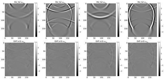
Figure 5.
Wavefield separation results from the U-Net for the snapshot shown in Figure 4. The top row depicts ux_qp, ux_qs, uz_qp, and uz_qs, and the bottom row illustrates the residual maps (scaled by a factor of three for clarity) relative to the ground truth. Higher residuals appear near complex reflections and interfaces.
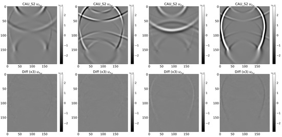
Figure 6.
Wavefield separation results from the cross-attention U-Net for the same snapshot. The top row shows ux_qp, ux_qs, uz_qp, and uz_qs, while the bottom row presents the residual maps (also scaled by a factor of three). Compared to Figure 5, these predictions exhibit fewer artifacts and more accurate separation across all components.
3.2. Application to Larger Anisotropic Models
To evaluate the scalability and robustness of the trained network, the cross-attention U-Net was first tested on a substantially larger subset of the same BP model. While the training region was limited to 200 × 200 patches, the larger domain considered here spans 1936 × 562 grid points and includes boundary extensions to reduce reflection artifacts. To handle this increased domain without exceeding the GPU memory limits, a sliding-patch approach that is commonly used in image processing was employed [19]. This method divides the domain into partially overlapping patches, processes each patch independently, and merges the outputs through a smoothly tapered weighting function that prevents visible seams.
Figure 7 presents the wavefield separation results for the BP model, showing the input displacement fields (ux and uz) in the top row, ground truth qP and qS components (ux_qp, ux_qs, uz_qp, uz_qs) in the second row, predicted components in the third row, and difference maps in the bottom row. While the model successfully separates the wavefields across the expanded domain, the difference maps reveal some discrepancies between the predicted and ground truth components. These residuals indicate a modest decrease in performance compared to the results presented in Section 3.1, which is an expected trade-off when scaling to larger domains and implementing patch-based processing.
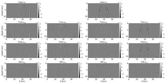
Figure 7.
Wavefield separation results on the larger BP model domain (1936 × 562) using the sliding-patch approach. Input displacement fields (top row: ux and uz), ground truth qP and qS components (second row: ux_qp, ux_qs, uz_qp, uz_qs), predicted components using the cross-attention U-Net (third row), and difference maps between the predicted and ground truth results (bottom row).
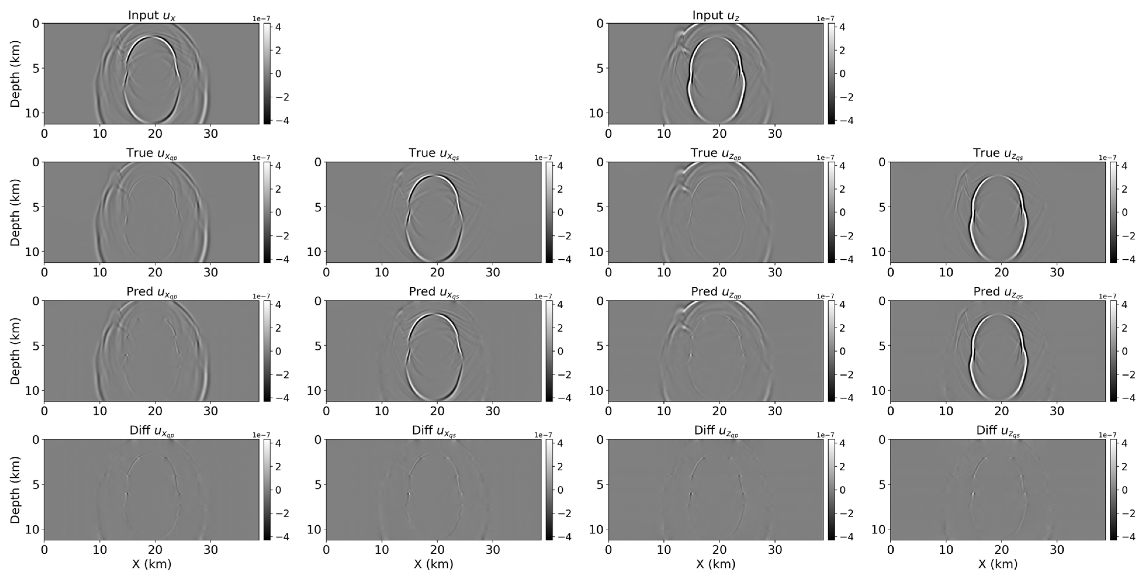
To further examine the network’s generalization capabilities, the same sliding-patch approach was applied to the Hess VTI (vertical transverse isotropy) model, with additional synthetic noise being injected into the wavefields. The noise was generated using a random Gaussian distribution, scaled by a relative amplitude factor up to 30% of the maximum absolute value in each snapshot. Although the network was trained exclusively on clean data, it demonstrated robust performance on this noisy dataset. As shown in the updated Figure 8, the cross-attention U-Net was able to produce coherent qP and qS components, even in the presence of noise and strong heterogeneity. Some residual artifacts were observed, particularly around high-contrast regions, but the decomposition quality remained largely consistent. These results indicate that the model can generalize to more complex data distributions beyond the training set and highlight its potential for application to real seismic datasets, where noise and heterogeneity are prevalent.

Figure 8.
Wavefield separation results on the noisy Hess VTI model using the sliding-patch approach. Input displacement fields (top row: ux and uz) with added Gaussian noise, ground truth qP and qS components (second row: ux_qp, ux_qs, uz_qp, uz_qs), predicted components using the cross-attention U-Net (third row), and difference maps between the predicted and ground truth results (bottom row).
4. Discussion
While the proposed cross-attention U-Net shows promising results in elastic wavefield decomposition, several aspects require further consideration. One of the main challenges is the computational complexity that is introduced by the cross-attention mechanism. Since attention operations scale quadratically with input size, this can create a bottleneck for applications involving large seismic datasets. This limitation necessitates the exploration of optimization strategies such as sparse attention techniques, hierarchical attention implementations, or alternative attention mechanisms that can maintain performance while reducing the computational overhead.
Another area of concern is the model’s dependence on labeled training data. Unlike physics-based approaches, the proposed approach requires a considerable amount of labeled data for effective generalization. Although the use of low-rank approximations for generating labels has been effective in the current setting, this method may introduce potential bias due to the assumptions involved in the approximation. In particular, it is unclear how these labels generalize to complex real data, where assumptions may not hold. Investigating alternative label generation strategies, such as weak supervision or self-supervised learning, could help reduce such bias while improving model robustness.
Extending the method to three-dimensional wavefield decomposition is an important next step for real data applications. However, this also increases the computational and memory demands of the model. Future work should focus on improving the scalability for 3D domains, possibly by introducing hybrid attention architectures that combine local and global representations or by leveraging the structural characteristics of seismic data to reduce the processing overhead. In addition, inference with the trained network is considerably faster than conventional decomposition methods, such as low-rank approximations, which require intensive computation for each snapshot. Once training is complete, the model yields predictions almost instantly through a single forward pass, making it well suited for large-scale or time-sensitive applications.
In addition, when the model is applied to larger domains using a sliding-patch inference approach, some reduction in accuracy can be observed near patch boundaries. This appears to stem from the limited receptive field of the network, which is trained on relatively small patches (200 × 200) and may not capture long-range spatial dependencies effectively. This limitation becomes more noticeable when processing extended domains, as illustrated in Figure 7 and Figure 8. Potential improvements could include overlapping patch strategies with smooth blending, or the integration of global context modeling techniques such as attention modules that span wider spatial extents.
While the model performs well across different velocity structures and anisotropic characteristics, further development is needed to improve its performance in more complex geological settings. This could include incorporating physical constraints directly into the network architecture or loss function, helping the model align more closely with the underlying physics. Additionally, interpretability tools tailored to wavefields decomposition could offer useful insights into how the model makes decisions and support validation in practical scenarios.
5. Conclusions
This study presents a cross-attention enhanced U-Net architecture for elastic wavefield vector decomposition in anisotropic media. The method combines deep learning with a dual-branch encoder structure to process displacement components separately while maintaining their relationships through cross-attention mechanisms. The results show that the cross-attention mechanisms improve the decomposition quality, achieving better accuracy and fewer artifacts compared to conventional U-Net architectures. The model’s performance on larger domains and different geological settings, demonstrated through experiments with the BP and Hess VTI models, indicates its potential for practical seismic applications. The cross-attention U-Net effectively preserves physical relationships between displacement components while reducing the computational complexity compared to traditional methods that rely on solving the Christoffel equation.
Funding
This research was supported by a National Research Foundation of Korea (NRF) grant, funded by the Korea government (MSIT) (No. 2023-00212423) and was also supported by a research grant from the Gyeongsang National University in 2022.
Data Availability Statement
The original contributions presented in this study are included in the article. Further inquiries can be directed to the corresponding author(s).
Acknowledgments
The anonymous reviewers and the associated Editor are appreciated for their constructive comments that helped improve the quality of the manuscript. The 2007 BP anisotropic velocity benchmark dataset, created by Hemang Shah and provided courtesy of BP Exploration Operation Company Limited, was used for training purposes. The dataset is publicly available at https://wiki.seg.org/wiki/2007_BP_Anisotropic_Velocity_Benchmark, accessed on 1 April 2025. The Hess VTI migration benchmark dataset, generated using finite-difference modeling software developed by Hess Corporation, was used for model evaluation. The dataset is publicly accessible at https://wiki.seg.org/wiki/Hess_VTI_migration_benchmark, accessed on 1 April 2025.
Conflicts of Interest
The author declares no conflicts of interest.
References
- Yan, J.; Sava, P. Elastic wave-mode separation for VTI media. Geophysics 2009, 74, WB19–WB32. [Google Scholar] [CrossRef]
- Cheng, J.; Fomel, S. Fast algorithms for elastic wave-mode separation and vector decomposition using low-rank approximations. Geophysics 2014, 79, C97–C110. [Google Scholar] [CrossRef]
- Aki, K.; Richards, P.G. Quantitative Seismology, 2nd ed.; University Science Books: Sausalito, CA, USA, 2002. [Google Scholar]
- Dellinger, J.; Etgen, J. Wavefield separation in two-dimensional anisotropic media. Geophysics 1990, 55, 914–919. [Google Scholar] [CrossRef]
- Zhang, Q.; McMechan, G.A. 2D and 3D elastic wavefield vector decomposition in the wavenumber domain for VTI media. Geophysics 2010, 75, D13–D26. [Google Scholar] [CrossRef]
- Yan, J.; Sava, P. Improving the efficiency of elastic wave-mode separation for heterogeneous tilted transverse isotropic media. Geophysics 2011, 76, T65–T78. [Google Scholar] [CrossRef]
- Zhou, Y.; Wang, H. Efficient wave-mode separation in vertical transversely isotropic media. Geophysics 2017, 82, C35–C47. [Google Scholar] [CrossRef]
- Sripanich, Y.; Fomel, S.; Sun, J.; Cheng, J. Elastic wave-vector decomposition in heterogeneous anisotropic media. Geophys. Prospect. 2017, 65, 1231–1245. [Google Scholar] [CrossRef]
- Huang, H.; Wang, T.; Cheng, J. Elastic wave mode decomposition in anisotropic media with convolutional neural network. In Proceedings of the 82nd EAGE Annual Conference & Exhibition, European Association of Geoscientists & Engineers, Amsterdam, The Netherlands, 18–21 October 2021; pp. 1–5. [Google Scholar] [CrossRef]
- Sun, Z.; Gu, B.; Zhang, Y.; Zhang, S.; Yan, X. P/S wavefield separation using modified U-Net based on ConvNeXt architecture. J. Appl. Geophys. 2023, 217, 105185. [Google Scholar] [CrossRef]
- Kaur, H.; Fomel, S.; Pham, N. A fast algorithm for elastic wave-mode separation using deep learning with generative adversarial networks (GANS). J. Geophys. Res. Solid Earth 2021, 126, e2020JB021123. [Google Scholar] [CrossRef]
- Vaswani, A.; Shazeer, N.; Parmar, N.; Uszkoreit, J.; Jones, L.; Gomez, A.N.; Kaiser, Ł.; Polosukhin, I. Attention Is All You Need. In Proceedings of the 31st International Conference on Neural Information Processing Systems (NeurIPS 2017), Long Beach, CA, USA, 4–9 December 2017; pp. 5998–6008. [Google Scholar] [CrossRef]
- Carion, N.; Massa, F.; Synnaeve, G.; Usunier, N.; Kirillov, A.; Zagoruyko, S. End-to-End Object Detection with Transformers. In Proceedings of the European Conference on Computer Vision (ECCV), Virtual Event, 23–28 August 2020; pp. 213–229. Available online: https://arxiv.org/abs/2005.12872 (accessed on 19 February 2025).
- Ramesh, A.; Dhariwal, P.; Nichol, A.; Chu, C.; Chen, M. Hierarchical text-conditional image generation with clip latents. arXiv 2022, arXiv:2204.06125. [Google Scholar] [CrossRef]
- Ronneberger, O.; Fischer, P.; Brox, T. U-Net: Convolutional Networks for Biomedical Image Segmentation. In Proceedings of the International Conference on Medical Image Computing and Computer-Assisted Intervention (MICCAI 2015), Munich, Germany, 5–9 October 2015; pp. 234–241. Available online: https://arxiv.org/abs/1505.04597 (accessed on 19 February 2025).
- He, K.; Zhang, X.; Ren, S.; Sun, J. Deep Residual Learning for Image Recognition. In Proceedings of the IEEE Conference on Computer Vision and Pattern Recognition (CVPR), Las Vegas, NV, USA, 27–30 June 2016; pp. 770–778. Available online: https://arxiv.org/abs/1512.03385 (accessed on 19 February 2025).
- He, K.; Zhang, X.; Ren, S.; Sun, J. Delving Deep into Rectifiers: Surpassing Human-Level Performance on ImageNet Classification. In Proceedings of the IEEE International Conference on Computer Vision (ICCV), Santiago, Chile, 7–13 December 2015; pp. 1026–1034. Available online: https://arxiv.org/abs/1502.01852 (accessed on 19 February 2025).
- Kingma, D.P.; Ba, J.L. Adam: A method for stochastic optimization. In Proceedings of the 3rd International Conference on Learning Representations (ICLR), San Diego, CA, USA, 7–9 May 2015; pp. 1–15. [Google Scholar] [CrossRef]
- Efros, A.A.; Freeman, W.T. Image Quilting for Texture Synthesis and Transfer. In Proceedings of the 28th Annual Conference on Computer Graphics and Interactive Techniques (SIGGRAPH 2001), Los Angeles, CA, USA, 12–17 August 2001; pp. 341–346. [Google Scholar] [CrossRef]


Disclaimer/Publisher’s Note: The statements, opinions and data contained in all publications are solely those of the individual author(s) and contributor(s) and not of MDPI and/or the editor(s). MDPI and/or the editor(s) disclaim responsibility for any injury to people or property resulting from any ideas, methods, instructions or products referred to in the content. |
© 2025 by the author. Licensee MDPI, Basel, Switzerland. This article is an open access article distributed under the terms and conditions of the Creative Commons Attribution (CC BY) license (https://creativecommons.org/licenses/by/4.0/).