Abstract
Predicting the river discharge is essential for preparing effective measures against flood hazards or managing hydrological droughts. Despite mathematical modeling advancements, most algorithms have failed to capture the extreme values (especially the highest ones). In this article, we proposed a quantum neural networks (QNNs) approach for forecasting the river discharge in three scenarios. The algorithm was applied to the raw data series and the series without aberrant values. Comparisons with the results obtained on the same series by other neural networks (LSTM, BPNN, ELM, CNN-LSTM, SSA-BP, and PSO-ELM) emphasized the best performance of the present approach. The lower error between the recorded values and the predicted ones in the evaluation of maxima compared to the case of the competitors mentioned shows that the algorithm best fits the extremes. The most significant mean standard errors (MSEs) and mean absolute errors (MAEs) were 26.9424 and 4.8914, respectively, and the lowest R2 was 84.36%, indicating the good performances of the algorithm.
1. Introduction
Water resources are essential for human life; throughout history, rivers have been the nuclei of the places where civilizations were born. Floods are among the hazards that produce significant life losses annually [1,2]. Therefore, the analysis and modeling of river discharge is essential for limiting the negative impact of such hazards and taking prevention measures, among which plans in the case of disasters are essential [3,4,5,6,7].
Various techniques have been employed to describe the pattern of the river flow, for example, statistics-based approaches, including Box–Jenkins models [8,9,10,11,12], Generalized Linear Models (GLMs) [13], Generalized Additive Models (GAMs) [14], Generalized Additive Mixed Models (GAMMs) [15,16], and Weighted Regression [17]. Utilizing Artificial Intelligence (AI) techniques [18,19,20,21] in forecasting the river flow increased the models’ accuracy, given the ability of machine learning (ML) techniques to capture the high variability of the various data series, such as in medicine, cybersecurity, engineering, environmental sciences, decision making, economics, etc. [22,23,24,25,26,27,28,29]. Hybrid algorithms overperform in many cases compared to the single AI ones [30,31] in terms of the forecast. However, in most cases, the extremes are not well captured, impacting the neighboring values’ prediction.
The rapid development of quantum computing hardware has led to the parallel advancement of multiple technological approaches. Among these, superconducting circuits and ion trap technologies have demonstrated significant advantages and currently hold a leading position in the field [32,33]. Ion trap technology has exhibited remarkable performance in high-precision quantum gate operations, providing strong support for constructing large-scale and stable quantum computers. By confining single or multiple ions and precisely controlling their states using laser techniques, ion trap technology effectively reduces external interference. It also maintains qubit coherence, thereby enabling high-fidelity quantum logic gate operations [32,33].
In quantum simulation, quantum computers can simulate intricate quantum systems beyond the capabilities of classical computers. This enables in-depth studies of quantum many-body physics and quantum chemistry, facilitating research into high-temperature superconductivity mechanisms, novel drug design, and material discovery [33,34]. The quantum algorithms integrate the strengths of quantum and classical computing, leveraging quantum trials to achieve superior approximations compared to classical methods, with practical applications in logistics scheduling and financial risk management [33,35,36].
Quantum neural networks (QNNs) represent a fusion of quantum computing and neural networks, aiming to enhance neural network performance by harnessing quantum properties. The fundamental principle of QNNs involves using qubits to represent neuron states and employing quantum gate operations to facilitate information processing and transmission between neurons [37]. QNNs exploit quantum superposition and entanglement to enable more complex and efficient information processing. For instance, in a simple QNN model, the input quantum state undergoes a series of quantum gate transformations to produce an output state analogous to the computational process of neurons in classical networks [38]. In practical applications, QNNs exhibit unique advantages. QNNs outperform classical neural networks in image recognition tasks by effectively capturing intricate features within image data [39]. The superposition states of qubits allow simultaneous representation of multiple states, enabling QNNs to process high-dimensional data more comprehensively and improve recognition accuracy [40].
Applications of QNNs can be seen in chemistry [40], materials informatics [41], hardware security [42], times series forecasting [43,44], and weather prediction [45]. A review of the recent applications of QNNs is presented in [46].
This study applies quantum neural networks (QNNs) to river discharge prediction. Although classical neural network techniques have achieved significant success in this field, the core value of this research lies in exploring the feasibility of quantum intelligence methods in this domain and conducting an in-depth analysis of their predictive performance, mainly because the approaches using classical NNs failed to capture the extremes in the data series. The proposed approach is not only executable in quantum simulation environments on classical computers but also has the potential to be implemented on actual quantum hardware, leveraging unique quantum advantages such as ultrafast computation, parallel processing, and computational acceleration enabled by quantum superposition and entanglement. Results show significant performances of this approach in forecasting three data series.
2. Methodology and Data Series
2.1. Computational Experiment
The experimental environment is based on a high-performance computing system with an AMD RYZEN5 5500 processor (AMD, Santa Clara, CA, USA) and 24 GB of memory, ensuring computational efficiency and stability. In terms of software configuration, Anaconda was utilized as the package management and environment configuration tool, facilitating dependency management and version control of various software libraries. The experiments were conducted using Python 3.12, which offers enhanced performance optimization while maintaining compatibility.
For quantum computing simulations, we employed Qiskit, an open-source framework developed by IBM specifically designed for quantum computing research and applications. Qiskit provides a comprehensive suite of functionalities, including quantum circuit construction, quantum algorithm simulation, and hardware backend integration, effectively supporting the modeling and computational processes involved in quantum neural networks in this study. Furthermore, we optimized simulation parameters within the Qiskit environment to enhance computational efficiency. We leveraged scientific computing libraries such as NumPy and SciPy to improve numerical stability and computational performance. The computational environment established in this study ensures the effective implementation of quantum intelligence methods while providing a robust technical foundation for efficient model training.
2.2. Quantum Neural Network
2.2.1. Basic Concept of Quantum Neural Network
The Quantum Neural Network (QNN) is a computational model that integrates quantum computing and neural networks. It aims to leverage quantum computing properties such as quantum superposition, quantum entanglement, and quantum parallelism to enhance the expressiveness and computational efficiency of neural networks. QNNs replace classical neural networks’ traditional weights and activation functions with Variational Quantum Circuits (VQCs) to perform learning tasks [37].
The qubit is the fundamental unit that carries information, whose state can be described by
where α and β are complex numbers whose sum of squared modulus is 1.
|ϕ⟩ = α |0⟩ + β |1⟩
Quantum data includes the quantum states (|0⟩, |1⟩), superposition states (e.g., |0⟩ + |1⟩), and entangled states. Quantum registers are used to organize the data.
Quantum Gates (e.g., Hadamard, Pauli, CNOT, Toffoli) have the role of manipulating the qubits for computation. For example, the U gate performs a single-qubit rotation, whereas Rx (Ry, and Rz) performs a rotation around the Ox (Oy, and Oz) axis [47].
In the QNN structure, input data are first mapped to the quantum state space and then transformed through parameterized quantum gate operations. The final computation results are obtained via quantum measurement, and classical optimization methods are used to adjust circuit parameters to minimize the loss function, thus completing the training process. Compared to classical neural networks, QNNs take advantage of the unique physical properties of quantum computers, which may provide computational acceleration and superior feature mapping capabilities in specific tasks.
2.2.2. Structure of Quantum Neural Networks
A QNN consists of three core components:
- (1)
- Quantum Feature Mapping (Data Encoding)
Before processing, classical input data must be mapped to a quantum state. This process is known as Quantum Feature Mapping, which uses quantum gate operations to embed the input data as quantum state parameters [48]. For example, for a one-dimensional input x, encoding can be performed using rotation gates (Ry, Rz):
In multi-qubit systems, entanglement-based mapping (such as ZZ feature mapping) can be used to enhance data separability [38]:
where H represents the Hamiltonian, typically constructed using Pauli-Z interaction terms [49].
Entanglement is a quantum correlation where the particle’s state is linked to another particle’s state (no matter the distance between them). Therefore, the state of one entangled particle determines the other particle’s state [47].
- (2)
- Measurement and Optimization
Once QNN computations are complete, quantum measurement is performed to extract the computational results. Common measurement methods include:
- Pauli-Z measurement: Computing the expectation value ⟨Z⟩ for classification or regression tasks [50]:
- Shot-based Sampling: Since quantum measurements are probabilistic, multiple measurements are required to obtain a stable output.
The measured results are used in the loss function, and classical optimization algorithms such as Gradient Descent [51], L-BFGS-B (quasi-Newton method) [52], and COBYLA [53,54] (constrained optimization) are employed to fine-tune the circuit parameters, improving the model’s fit to the target data.
2.2.3. Computational Process of QNN
The computational process of a QNN consists of the following steps [55,56]:
- (a)
- Mapping Classical Data to Quantum States. The input data x are transformed into a quantum state using a Quantum Feature Mapping Circuit:
- (b)
- Quantum Circuit Processing. The Variational Quantum Circuit (VQC) applies quantum gate operations to the quantum state:where U(θ) is composed of multiple trainable parameterized quantum gates.
- (c)
- The expectation value of quantum states is measured:Measurement results are used for loss function calculation.
- (d)
- Parameter Optimization. Classical optimization algorithms update the quantum circuit parameters, using Equation (8),where L is the loss function, η is the learning rate.
- (e)
- Training and Convergence. The above process is iterated until the loss function (mean standard error—MSE, or mean absolute error—MAE) converges, leading to optimized parameters θ.
Quantum algorithms are a core component of quantum computing, designed to leverage the unique advantages of quantum computers to solve complex problems that are challenging for classical computers. These algorithms exploit quantum parallelism and coherence, achieving exponential acceleration over classical algorithms, thereby providing novel solutions in cryptography and number theory [32]. Quantum search algorithms, such as Grover’s, demonstrate unique advantages in searching unstructured databases by achieving quadratic speedup. By utilizing quantum superposition and interference, Grover’s algorithm enhances search efficiency and holds potential applications in information retrieval and optimization problems [32].
The three main challenges of QNN are quantum decoherence, error correction, and scalability. Decoherence leads to computation errors. Therefore, the computation should be completely executed in the qubit coherence time, which is relatively short. The errors correction is based on the topological approach. Quantum computing may scale better than the classical one, but achieving this is challenging due to limited qubit connections. Moreover, most scaling techniques for classical computers do not apply to current quantum computers. In summary, quantum computing presents significant challenges for scalability [57].
2.3. Study Area and Data Series
The Buzău River is a significant watercourse in southeastern Romania, flowing through the Curvature Carpathians and the Buzău Plateau to the Siret River. Its catchment (Figure 1) covers 5264 km2 and includes diverse landscapes, from the mountains in the Curvature Carpathians to the lower plateau regions. The mean elevation of the Buzău River is 1043 m above sea level.
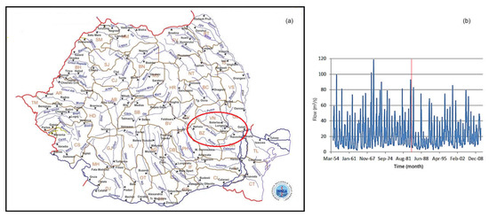
Figure 1.
(a) The Romanian map and the Buzău catchment—inside the ellipse in red, and (b) the data series (S). The vertical red line represents the delimitation between the two series—S1 (before 1 January 1984) and S2 (January 1984).
This variation in terrain affects the river’s flow, with heavy rainfall in the higher regions often causing significant runoff during storms. The river basin is located within a temperate continental climate zone, which results in distinct seasonal shifts in temperature, precipitation, and runoff. Over 80% of the river’s annual flow comes from the basin’s upper reaches, especially from tributaries upstream of the town of Nehoiu. The region has experienced severe flooding, particularly in the mid-20th century, with the most notable occurring in 1975 when the Buzău River reached a peak discharge of 2100 m3/s. These floods prompted the development of flood control infrastructure, including the construction of dams. To address flood risks, regulate the river’s flow, and provide electricity, the Siriu Dam was built on the Buzău River (partially put into function on 1 January 1984). Its apparition has been instrumental in reducing flood risks and altering the river’s natural flow, improving surrounding communities’ life conditions [58,59].
The studied series is formed by monthly river flow from January 1955 to December 2010. For modeling purposes, the entire series, denoted by S, was divided into the subseries S1 (January 1955–December 1983) and S2 (covering the rest of the period). The series were standardized before applying QNN. Each series (S, S1, and S2) was divided into training and test sets. The training sets were before January 2005 (before January 1984) for S (for S1) and between January 1984 and December 2005 for S2. The test one was the same in all cases, i.e., after January 2006. It is the series for which the forecast was conducted after the model learned the data on the training sets. Modeling was also performed on the same series after removing the anomalies, which are mainly the extreme values with respect to their neighbors (Figure 2). These series will be denoted by So, S1o, and S2o. We shall not present the methodology utilized for anomaly detection because it is presented in detail in our articles [60,61]. The statistical analysis of the series and an extended description of the study region can be found in [62].
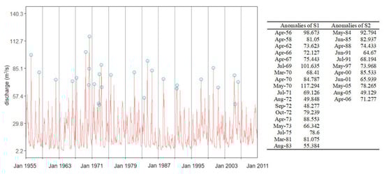
Figure 2.
S series and anomalies represented by blue circles. The table contains the values of anomalies and the corresponding apparition month [63].
Anomalies are occurrences in a dataset that are in some way unusual and do not fit the general patterns. In hydrology, they are generally associated with high water discharges (appearing in the case of high precipitations, for example) with extreme values (maxima). When interested only in extremes, the theory of extreme values can be applied. In hydrology, the Peak over Threshold (POT) [64] is generally used to model the distributions of extreme values and find the return period. However, only the values above a certain threshold are utilized in such a case. The anomalies should be kept when determining a model for the entire data series. In this article, in the first stage, the models were built in each scenario without eliminating the extremes. In the second stage, we removed the outliers and reran the algorithm to address the algorithm’s performance.
3. Results and Discussion
3.1. Results for the Raw Series
Figure 3 presents the real and fitted model for S series, on the training (Figure 3a) and test (Figure 3b) sets, together with the variation of the objective function (Figure 3c).
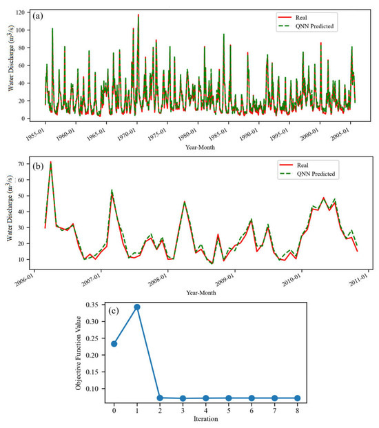
Figure 3.
The QNN model for S (a) on the training and (b) test sets. (c) The evolution of the objective function during the training (8 iterations).
We notice the quick convergence of the objective function to a value under 0.4, which, together with the chart from Figure 3a, indicates a good algorithm performance on the training set. Figure 3b shows that the simulated series has the same shape as the recorded one, except for a few periods when the actual series is increasing while the simulated one is decreasing (e.g., 2007-06, 2009-01, 2009-02, etc.). In most cases, the bias between the forecast series and the recorded one is positive, indicating a slight overestimation of the raw data series. We also remark that there is a very good fit of the highest values in the test series. Comparisons of the training and test results indicate a better fit in the first case. In the second one, the highest bias is noticed in 2009-October and 2010-April, August, November, and December.
Figure 4 presents the results of QNN on S1.
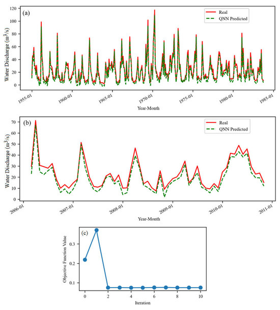
Figure 4.
The QNN model for S1 (a) on the training set and (b) test set. (c) The evolution of the objective function during the training (10 iterations).
The maximum value of the objective function was higher in this situation than for S, but it dropped under 0.5 after two iterations, remaining almost constant. The model did not very well fit the river’s discharge extreme values of the training set (Figure 4a), mainly underestimating them. The shapes of the raw and simulated series are similar on the test set (Figure 4b). The highest underestimated values of the recorded series are in March–April, August–October 2006, January–February, November 2008, etc.
Comparisons of Figure 3b and Figure 4b show a better performance of the model on S compared to that on S1, in the first case the extremes being better fitted. These results were somehow expected because, in the case of S, the training set contained values recorded before 1984 and a part after January 1984, whereas in the case of S1, the training set was in the period before the river flow regularization, and the test set was recorded after that moment. Therefore, the inhomogeneity of the data series was higher when modeling S1.
Figure 5 illustrates the behavior of the simulated series against the recorded S2.
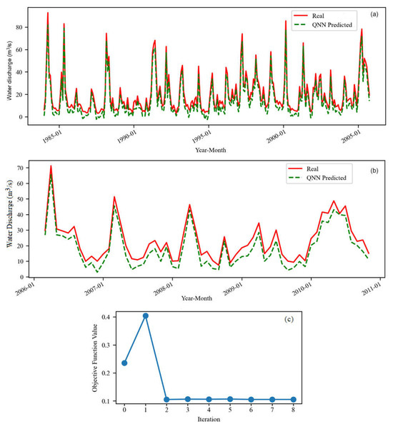
Figure 5.
The QNN model for S2 (a) on the training set and (b) test set. (c) The evolution of the objective function during the training (8 iterations).
Despite the homogeneity of the training and test sets (both belonging to the same period, after building the Siriu Dam), we notice that there are higher deviations of the simulated series from the registered one on the test set (Figure 5b) compared to the case of the entire series S (that contains values from both periods, before and after the change in the water discharge regimen). The objective function stabilizes at about 0.1, a higher value compared to the cases of S and S1, indicating a worse fit of the test series of S2. Moreover, the training and test datasets are both underestimated. This behavior was unexpected because both sets (training and test) belonged to the same period (after 1984). The result is opposite to those obtained using other algorithms on the same data series [60,63,65].
3.2. Results for the Series After the Anomalies Removal
The same algorithm was applied to the series after removing the values presented in Figure 2 to evaluate the algorithm’s behavior in a series with lower variability. The results are represented in Figure 6 for the So series, Figure 7 for S1o, and Figure 8 for S2o.
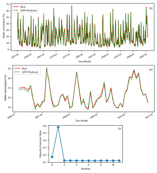
Figure 6.
QNN model for So (a) on the training set and (b) test set. (c) The evolution of the objective function during the training (11 iterations).
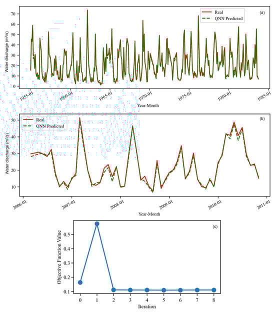
Figure 7.
The QNN model for S1o on (a) the training set and (b) test set. (c) The evolution of the objective function during the training (8 iterations).
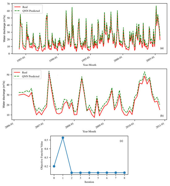
Figure 8.
The QNN model for S2o (a) on the training set and (b) test set. (c) The evolution of the objective function during the training (8 iterations).
The objective function computed during the training process for So levels off at the second iteration at a value higher than for S. On the training set, the QNN better fit So, except for the first three values, where a significant deviation is noticed.
As can be seen in Figure 7c (Figure 8c), the objective function for S1o (S2o) leveled off at higher (much lower) values than for S1 (S2).
For S1o, the extremes are well captured in both the training and testing sets. At the beginning of 2006 and the middle of 2007, a few significant differences between the measured and simulated series exist.
In the case of S2o, the predicted values are higher than the recorded ones, with a bigger bias than in the cases of S and S1o. However, the forecast series and the registered one have the same shape, indicating the model’s capacity to catch all kinds of values (high or small) well. Comparisons of Figure 6, Figure 7 and Figure 8 show a lower accuracy of S2o compared to So and S1o. A similar remark can be made by analyzing Figure 3, Figure 4 and Figure 5.
3.3. Results Comparisons
Table 1 contains comparisons of the modeling results. The models’ evaluation was based on the MAE, MSE, and R2. With respect to MAE, the best results on the training set were obtained for S and So. The model built for So (S1o, and S2o, respectively) is better than that for S (S1, and S2, respectively). The models performed better on the test series S, S1, and S2o compared to the training sets, whereas for the rest of the models, the best results were those on the training sets.

Table 1.
Comparison of the models’ performance.
The MAE and MSE are significantly higher when modeling the raw data series than those without aberrant values.
Opposite, R2 is lower in the same case. In terms of R2, all the models have a very high accuracy, the lowest being that of the S2 model. These observations indicate a worse fit of the initial series, presenting a higher variability than those without aberrants. Overall, the best models were those for So and S1o, followed by those for S and S2o, even though we expected the best accuracy for S2o given that the training and test sets belong to the period after building the dam and removing the aberrant values.
The run time and the corresponding number of epochs are presented in the last two columns of Table 1. The smallest were those associated with S2o, S2, and S1o (the shortest series), and the highest were those for So (not S, as expected given the length).
The following compares the results of the previous studies [60,65] performed for the same series and the same training and test sets.
- ➢
- On the S series,
- On the training set, the lowest MAE, 5.7250, was obtained using a hybrid Sparrow Search Algorithm–Backpropagation Neural Network (SSA-BP), and on the test set, 4.2351, by a Convolutional Neural Network–Long Short-Term Memory (CNN-LSTM).
- On the training set, the lowest MSE, 80.5765, resulted from an Echo State Network (ESN) algorithm, and on the test set, 32.4993, from SSA-BP.
- On the training set, the highest R2, 0.9976, resulted after fitting a Sparrow Search Algorithm–Echo State Network (SSA-ESN) model, and on the test set, 0.9983, after using a Long Short-Term Memory (LSTM) model.
- ➢
- On the S1 series,
- On the training set, the lowest MAE, 6.5177, was obtained using CNN-LSTM, and on the test set, 4.4784, by the same algorithm.
- On the training set, the lowest MSE, 102.9393, resulted from an ESN algorithm, and on the test set, 39.7982, from CNN-LSTM.
- On the training and test sets, the highest R2, 0.9899 and 0.9917, respectively, resulted from fitting an LSTM model.
- ➢
- On the S2 series,
- On the training and test sets, the lowest MAEs, 4.7433 and 3.5245, respectively, were obtained using CNN-LSTM.
- On the training set, the lowest MSE, 57.3421, resulted from an SSA-ESN algorithm, and on the test set, 29.8323, from CNN-LSTM.
- On both training and test sets, the highest R2, 0.9992 and 0997, respectively, resulted from an LSTM model fitting.
The values of the goodness of fit indicators presented above indicate a lower performance of the classical NN algorithms compared to the QNN, at least in terms of MSE and MAE. Similar comparisons can be made for the series So, So1, and So2, leading to a similar conclusion. Therefore, the proposed approach shows its potential in modeling the river discharge, even in the case of inhomogeneous data series.
4. Conclusions
In this study, we explored the performance of QNNs in modeling river discharge. It was shown that QNNs successfully captured extreme values. This study demonstrates that removing the aberrant values enhances the prediction performance, particularly in S and S1 datasets. The So model achieves the highest prediction accuracy, followed by So1. Modeling S2 and S2o remains more challenging, despite the smaller series length and the appurtenance of both subsets utilized for the training and test to the same period, i.e., after building the Siriu Dam.
Compared to classical NNs, the QNN models outperformed all the algorithms utilized in the previous studies on the same data series, emphasizing the quantum algorithm’s computational efficiency. Given these results, we intend to extend this study using other quantum algorithms, hoping to find better models for S2 for which the actual results are promising but can be improved. Moreover, testing QNNs on different hydrological datasets and optimizing their structure should be further explored.
Author Contributions
Conceptualization, L.Z. and A.B.; methodology, L.Z.; software, L.Z.; validation, L.Z. and A.B.; formal analysis, A.B.; investigation, L.Z. and A.B.; resources, L.Z.; data curation, A.B.; writing—original draft preparation, L.Z. and A.B.; writing—review and editing, A.B.; visualization, L.Z.; supervision, A.B.; project administration, A.B.; funding acquisition, A.B. All authors have read and agreed to the published version of the manuscript.
Funding
The research received no external fundings.
Institutional Review Board Statement
Not applicable.
Informed Consent Statement
Not applicable.
Data Availability Statement
Data will be available on request from the correspondence author.
Conflicts of Interest
The authors declare no conflicts of interest.
References
- Rentschler, J.; Salhab, M.; Jafino, B.A. Flood exposure and poverty in 188 countries. Nat. Commun. 2022, 13, 3527. [Google Scholar] [CrossRef]
- World Meteorological Organization. Provisional State of the Global Climate in 2022; World Meteorological Organization: Geneva, Switzerland, 2022; Available online: https://www.rmets.org/sites/default/files/2022-11/provisional_state_of_the_climate_2022_1_november_for_cop27_2.pdf (accessed on 4 April 2025).
- Serdar, M.Z.; Ajjur, S.B.; Al-Ghamdi, S.G. Flood susceptibility assessment in arid areas: A case study of Qatar. Sustainability 2022, 14, 9792. [Google Scholar] [CrossRef]
- Waleed, M.; Sajjad, M. Advancing flood susceptibility prediction: A comparative assessment and scalability analysis of machine learning algorithms via artificial intelligence in high-risk regions of Pakistan. J. Flood Risk Manag. 2025, 18, e13047. [Google Scholar] [CrossRef]
- Bărbulescu, A.; Maftei, C.E. Evaluating the Probable Maximum Precipitation. Case study from the Dobrogea region, Romania. Rom. Rep. Phys. 2023, 75, 704. [Google Scholar] [CrossRef]
- Popescu-Bodorin, N.; Bărbulescu, A. A ten times smaller version of CPC Global Daily Precipitation Dataset for parallel distributed processing in Matlab and R. Rom. Rep. Phys. 2024, 76, 703. [Google Scholar]
- Zhao, G.; Pang, B.; Xu, Z.; Peng, D.; Xu, L. Assessment of urban flood susceptibility using semi-supervised machine learning model. Sci. Total Environ. 2019, 659, 940–949. [Google Scholar] [CrossRef]
- Valipour, M.; Banihabib, M.E.; Behbahani, S.M.R. Comparison of the ARMA, ARIMA, and the autoregressive artificial neural network models in forecasting the monthly inflow of Dez dam reservoir. J. Hydrol. 2013, 476, 433–441. [Google Scholar] [CrossRef]
- Phan, T.-T.-H.; Nguyen, X.H. Combining statistical machine learning models with ARIMA for water level forecasting: The case of the Red river. Adv. Water Resour. 2020, 142, 103656. [Google Scholar] [CrossRef]
- Zhang, X.; Wu, X.; Zhu, G.; Lu, X.; Wang, K. A seasonal ARIMA model based on the gravitational search algorithm (GSA) for runoff prediction. Water Supply 2022, 22, 6959–6977. [Google Scholar] [CrossRef]
- Subha, J.; Saudia, S. Robust Flood Prediction Approaches Using Exponential Smoothing and ARIMA Models. In Artificial Intelligence and Sustainable Computing; Pandit, M., Gaur, M.K., Kumar, S., Eds.; Springer: Singapore, 2023; pp. 457–470. [Google Scholar]
- Alonso Brito, G.R.; Rivero Villaverde, A.; Lau Quan, A.; Ruíz Pérez, M.E. Comparison between SARIMA and Holt–Winters models for forecasting monthly streamflow in the western region of Cuba. SN Appl. Sci. 2021, 3, 671. [Google Scholar] [CrossRef]
- Yang, C.; Chandler, R.E.; Isham, V.S. Spatial-temporal rainfall simulation using generalized linear models. Water Resour. Resear. 2005, 41, W11415. [Google Scholar] [CrossRef]
- Rima, L.; Haddad, K.; Rahman, A. Generalised Additive Model-Based Regional Flood Frequency Analysis: Parameter Regression Technique Using Generalised Extreme Value Distribution. Water 2025, 17, 206. [Google Scholar] [CrossRef]
- Iddrisu, W.A.; Nokoe, K.S.; Luguterah, A.; Antwi, E.O. Generalized Additive Mixed Modelling of River Discharge in the Black Volta River. Open J. Stat. 2017, 7, 621–632. [Google Scholar] [CrossRef][Green Version]
- von Brömssen, C.; Fölster, J.; Kyllmar, K.; Bierosa, M. Modeling Complex Concentration-Discharge Relationships with Generalized Additive Models. Environ. Model. Assess. 2023, 28, 925–937. [Google Scholar] [CrossRef]
- Hirsch, R.M.; Moyer, D.L.; Archfield, S.A. Weighted Regressions on Time, Discharge, and Season (WRTDS), with an Application to Chesapeake Bay River Inputs. J. Am. Water Res. Assoc. 2010, 46, 857–880. [Google Scholar] [CrossRef] [PubMed]
- Ahmed, M.A.; Li, S.S. Machine Learning Model for River Discharge Forecast: A Case Study of the Ottawa River in Canada. Hydrology 2024, 11, 151. [Google Scholar] [CrossRef]
- Shabbir, M.; Chand, S.; Iqbal, F. A novel hybrid framework to model the relationship of daily river discharge with meteorological variables. Meteorol. Hydrol. Water Manag. 2023, 11, 70–94. [Google Scholar] [CrossRef]
- Zanial, W.N.C.W.; Malek, M.B.A.; Reba, M.N.M.; Zaini, N.; Ahmed, A.N.; Sherif, M.; Elsafie, A. River flow prediction based on improved machine learning method: Cuckoo Search-Artificial Neural Network. Appl. Water Sci. 2023, 13, 28. [Google Scholar] [CrossRef]
- Ni, L.; Wang, D.; Singh, V.P.; Wu, J.; Wang, Y.; Tao, Y.; Zhang, J. Streamflow and rainfall forecasting by two long short-term memory-based models. J. Hydrol. 2019, 583, 124296. [Google Scholar] [CrossRef]
- Dragomir, F.-L. Artificial intelligence techniques cybersecurity. In Proceedings of the International Scientific Conference STRATEGIES XXI, Bucharest, Romania, 27–28 April 2017; pp. 147–152. [Google Scholar]
- Rajkomar, A.; Dean, J.; Kohane, I. Machine Learning in Medicine. N. Engl. J. Med. 2019, 380, 1347–1358. [Google Scholar] [CrossRef]
- Dragomir, F.-L. Information system for macroprudential policies. Acta Univ. Danubius. Œconomica 2025, 21, 48–57. [Google Scholar]
- Simeone, O. Machine Learning in Engineering; Cambridge University Press: Cambridge, MA, USA, 2022. [Google Scholar]
- Shi, Y.-F.; Yang, Z.X.; Ma, S.; Kang, P.-L.; Shang, C.; Hu, P.; Liu, Z.-P. Machine Learning for Chemistry: Basics and Applications. Engineering 2023, 27, 70–83. [Google Scholar] [CrossRef]
- Bărbulescu, A.; Dumitriu, C.Ș. About the long-range dependence of cavitation effect on a copper alloy. Rom. J. Phys. 2024, 69, 904. [Google Scholar]
- Zhang, H.; Liu, Y.; Zhang, C.; Li, N. Machine Learning Methods for Weather Forecasting: A Survey. Atmosphere 2025, 16, 82. [Google Scholar] [CrossRef]
- Gogas, P.; Papadimitriou, T. Machine Learning in Economics and Finance. Comput. Econ. 2021, 57, 1–4. [Google Scholar] [CrossRef]
- Samantaray, S.; Sahoo, A.; Agnihotri, A. Prediction of Flood Discharge Using Hybrid PSO-SVM Algorithm in Barak River Basin. MethodsX 2023, 10, 102060. [Google Scholar] [CrossRef]
- Fathian, F.; Mehdizadeh, S.; Sales, A.K.; Safari, M.J.S. Hybrid models to improve the monthly river flow prediction: Integrating artificial intelligence and non-linear time series models. J. Hydrol. 2019, 575, 1200–1213. [Google Scholar] [CrossRef]
- Nielsen, M.A.; Chuang, I.L. Quantum Computation and Quantum Information: 10th Anniversary Edition; Cambridge University Press: Cambridge, MA, USA, 2010. [Google Scholar]
- Preskill, J. Quantum computing in the NISQ era and beyond. Quantum 2018, 2, 79. [Google Scholar] [CrossRef]
- Lloyd, S. Universal quantum simulators. Science 1996, 273, 1073–1078. [Google Scholar] [CrossRef]
- Farhi, E.; Goldstone, J.; Gutmann, S. A quantum approximate optimization algorithm. arXiv 2014, arXiv:1411.4028. [Google Scholar] [CrossRef]
- McClean, J.R.; Romero, J.; Babbush, R.; Aspuru-Guzik, A. The theory of variational hybrid quantum—Classical algorithms. New J. Phys. 2016, 18, 023023. [Google Scholar] [CrossRef]
- Biamonte, J.; Wittek, P.; Pancotti, N.; Rebentrost, P.; Wiebe, N.; Lloyd, S. Quantum machine learning. Nature 2017, 549, 195–202. [Google Scholar] [CrossRef]
- Cao, Y.; Romero, J.; Kieferová, M.; Shen, Z.; Babbush, R.; Aspuru-Guzik, A. Quantum-Enhanced machine learning. NPJ Quantum Inform. 2019, 5, 28. [Google Scholar]
- Kharsa, R.; Bouridane, A.; Amira, A. Advances in Quantum Machine Learning and Deep Learning for Image Classification: A Survey. Neurocomputing 2023, 560, 126843. [Google Scholar] [CrossRef]
- Schuld, M.; Sinayskiy, I.; Petruccione, F. Quantum machine learning in chemistry. J. Chem. Sci. 2018, 130, 1291–1306. [Google Scholar]
- Hirai, H. Practical application of quantum neural network to materials informatics. Sci. Rep. 2024, 14, 8583. [Google Scholar] [CrossRef]
- Beaudoin, C.; Kundu, S.; Topaloglu, R.O.; Ghosh, S. Quantum Machine Learning for Material Synthesis and Hardware Security. In Proceedings of the 41st IEEE/ACM International Conference on Computer-Aided Design ICCAD ’22, Dan Diego, CA, USA, 30 October–3 November 2022; p. 120. [Google Scholar]
- Azevedo, C.R.B.; Ferreira, T.A. The Application of Qubit Neural Networks for Time Series Forecasting with Automatic Phase Adjustment Mechanism. Available online: https://www.dcc.fc.up.pt/~ines/enia07_html/pdf/27825.pdf (accessed on 5 April 2025).
- Balakrishnan, D.; Mariappan, U.; Raghavendra, P.G.M.; Reddy, P.K.; Dinesh, R.L.N.; Jabiulla, S.B. Quantum Neural Network for Time Series Forecasting: Harnessing Quantum Computing’s Potential in Predictive Modeling. In Proceedings of the 2023 2nd International Conference on Futuristic Technologies (INCOFT), Belagavi, India, 24–26 November 2023; pp. 1–7. [Google Scholar]
- Safari, A.; Ghavifekr, A.A. Quantum Neural Networks (QNN) Application in Weather Prediction of Smart Grids. In Proceedings of the 2021 11th Smart Grid Conference (SGC), Tabriz, Iran, 7–9 December 2021; pp. 1–6. [Google Scholar]
- Jeswal, S.K.; Chakraverty, S. Recent Developments and Applications in Quantum Neural Network: A Review. Arch. Computat. Methods Eng. 2019, 26, 793–807. [Google Scholar] [CrossRef]
- Rath, M.; Date, H. Quantum data encoding: A comparative analysis of classical-to-quantum mapping techniques and their impact on machine learning accuracy. EPJ Quantum Technol. 2024, 11, 72. [Google Scholar] [CrossRef]
- Ranga, D.; Rana, A.; Prajapat, S.; Kumar, P.; Kumar, K.; Vasilakos, A.V. Quantum Machine Learning: Exploring the Role of Data Encoding Techniques, Challenges, and Future Directions. Mathematics 2024, 12, 331. [Google Scholar] [CrossRef]
- Djordjevic, I. Quantum Information Processing and Quantum Error Correction; Academic Press: Cambridge, MA, USA; Elsevier: Amsterdam, The Netherlands, 2012. [Google Scholar]
- Carleo, G.; Cirac, J.I.; Gull, S.; Martin-Delgado, M.A.; Troyer, M. Solving the quantum many-body problem with artificial neural networks. Science 2017, 355, 602–606. [Google Scholar] [CrossRef]
- Polyak, B. Introduction to Optimization. 1987. Available online: https://www.researchgate.net/profile/Boris-Polyak-2/publication/342978480_Introduction_to_Optimization/links/5f1033e5299bf1e548ba4636/Introduction-to-Optimization.pdf (accessed on 15 February 2025).
- Chen, H.; Wu, H.-C.; Chan, S.-C.; Lam, W.-H. A Stochastic Quasi-Newton Method for Large-Scale Nonconvex Optimization with Applications. IEEE Trans. Neural Netw. Learn. Syst. 2020, 31, 4776–4790. [Google Scholar] [CrossRef]
- Powell, M.J.D. A direct search optimization method that models the objective and constraint functions by linear interpolation. In Advances in Optimization and Numerical Analysis; Gomez, S., Hennart, J.-P., Eds.; Kluwer Academic: Dordrecht, The Netherlands, 1994; pp. 51–67. [Google Scholar]
- COBYLA. Available online: https://qiskit-community.github.io/qiskit-algorithms/stubs/qiskit_algorithms.optimizers.COBYLA.html (accessed on 15 February 2025).
- Kwak, Y.; Yun, W.Y.; Jung, J.S.; Kim, J. Quantum Neural Networks: Concepts, Applications, and Challenges. arXiv 2021, arXiv:2108.01468. [Google Scholar] [CrossRef]
- Zhou, M.-G.; Liu, Z.-P.; Yin, H.-L.; Li, C.-L.; Xu, T.-K.; Chen, Z.-B. Quantum Neural Network for Quantum Neural Computing. Research 2023, 6, 0134. [Google Scholar] [CrossRef] [PubMed]
- Jadhav, A.; Rasool, A.; Gyanchandani, M. Quantum Machine Learning: Scope for real-world problems. Procedia Comp. Sci. 2023, 218, 2612–2625. [Google Scholar] [CrossRef]
- Chendeş, V. Water Resources in Curvature Subcarpathians. Geospatial Assessments; Editura Academiei Române: Bucharest, Romania, 2011; (In Romanian with English Abstract). [Google Scholar]
- The Arrangement of the Buzău River. Available online: https://www.hidroconstructia.com/dyn/2pub/proiecte_det.php?id=110&pg=1 (accessed on 17 October 2023). (In Romanian).
- Zhen, L.; Bărbulescu, A. Echo State Network and Sparrow Search: Echo State Network for Modeling the Monthly River Discharge of the Biggest River in Buzău County, Romania. Water 2024, 16, 2916. [Google Scholar] [CrossRef]
- Bărbulescu, A.; Dumitriu, C.S.; Ilie, I.; Barbeş, S.-B. Influence of Anomalies on the Models for Nitrogen Oxides and Ozone Series. Atmosphere 2022, 13, 558. [Google Scholar] [CrossRef]
- Mocanu-Vargancsik, C.; Tudor, G. On the linear trends of a water discharge data under temporal variation. Case study: The upper sector of the Buzău river (Romania). Forum Geogr. 2020, XIX, 37–44. [Google Scholar] [CrossRef]
- Bărbulescu, A.; Zhen, L. Forecasting the River Water Discharge by Artificial Intelligence Methods. Water 2024, 16, 1248. [Google Scholar] [CrossRef]
- Naess, A. Applied Extreme Value Statistics; Springer: Cham, Switzerland, 2024. [Google Scholar]
- Zhen, L.; Bărbulescu, A. Comparative Analysis of Convolutional Neural Network-Long Short-Term Memory, Sparrow Search Algorithm-Backpropagation Neural Network, and Particle Swarm Optimization-Extreme Learning Machine Models for the Water Discharge of the Buzău River, Romania. Water 2024, 16, 289. [Google Scholar] [CrossRef]


Disclaimer/Publisher’s Note: The statements, opinions and data contained in all publications are solely those of the individual author(s) and contributor(s) and not of MDPI and/or the editor(s). MDPI and/or the editor(s) disclaim responsibility for any injury to people or property resulting from any ideas, methods, instructions or products referred to in the content. |
© 2025 by the authors. Licensee MDPI, Basel, Switzerland. This article is an open access article distributed under the terms and conditions of the Creative Commons Attribution (CC BY) license (https://creativecommons.org/licenses/by/4.0/).