Improved Deep Convolutional Generative Adversarial Network for Data Augmentation of Gas Polyethylene Pipeline Defect Images

Abstract

Gas polyethylene (PE) pipes have an become essential component of the urban gas pipeline network due to their long service life and corrosion resistance. To prevent safety incidents, regular monitoring of gas pipelines is crucial. Traditional inspection methods face significant challenges, including low efficiency, high costs, and limited applicability. Machine vision-based inspection methods have emerged as a key solution to these issues. Despite this, the method also encounters the problem of scarcity of defect samples and uneven data distribution in gas pipeline defect detection. For this reason, an improved Deep Convolutional Generative Adversarial Network (DCGAN) is proposed. By integrating the Minibatch Discrimination (MD), Spectral Normalization (SN), Self-Attention Mechanism (SAM) and Two-Timescale Update Rule (TTUR), the proposed approach overcomes the original DCGAN’s limitations, including mode collapse, low resolution of generated images, and unstable training, the data augmentation of defective images inside the pipeline is realized. Experimental results demonstrate the superiority of the improved algorithm in terms of image generation quality and diversity, while the ablation study validates the positive impact of the improvement in each part. Additionally, the relationship between the number of augmented images and classification accuracy, showing that classifier performance improved across all scenarios when generated defect images were included. The findings indicate that the images produced by the improved model significantly enhance defect detection accuracy and hold considerable potential for practical application.

1. Introduction

In the context of “Dual Carbon”, renewable energy is increasingly becoming a dominant component of the energy mix. Natural gas, as a clean and efficient fossil fuel, is essential for improving the energy mix and supporting the shift to cleaner energy sources. Pipeline transportation, one of the five major transportation modes, is the primary means of natural gas delivery [1,2,3]. Among the various pipeline materials, PE pipelines offer advantages such as cost-effectiveness, wear and corrosion resistance, and long service life. As a result, they are gradually replacing traditional steel pipelines and are widely used in the construction of gas pipeline networks [4]. PE pipelines are typically buried underground and subject to uncontrollable factors such as changes in underground temperature, foundation settlement, termite infestation, and stress effects. These conditions may develop defects such as structural aging, deformation, cracks, and dislocation at pipe joints, which can lead to serious risks such as gas leaks, fires, explosions, and other hazardous events, posing a significant threat to public safety [5,6,7,8]. Therefore, regular inspection and maintenance of gas polyethylene pipelines are essential to mitigate safety risks.

In gas pipeline defect detection, conventional non-destructive testing methods include ultrasonic testing, X-ray, infrared thermal imaging and machine vision methods [9]. Due to factors such as pipe material and inspection costs, ultrasonic testing, X-ray, and infrared thermal imaging are predominantly used for inspecting metal pipes [10,11,12]. The machine vision method, on the other hand, is fast, reduces inspection costs and workload, is unaffected by pipe material, and can be a comprehensive inspection of the internal surface of the pipe’s internal surface, structural deformations, and other defects [13,14].

In the field of machine vision, deep learning has been extensively applied to tasks such as image classification and object detection. However, data are crucial for training models, and the high cost and privacy concerns associated with collecting data on defects in gas polyethylene pipes often make it difficult to obtain and the lack of public datasets for researchers’ reference. This further complicates the training of deep learning models. Therefore, using data augmentation to increase the number of defect samples is important to improve the accuracy of internal defect detection of gas polyethylene pipelines. Data augmentation techniques offer an effective solution to the problem of limited samples by processing and expanding the existing data, enabling the limited data to generate value equivalent to that of a larger datasets. This enhances the model’s learning ability and is primarily categorized into two types: supervised and unsupervised [15].

Common methods for supervised data augmentation include geometric transformations, color transformations, CutMix, Mixup, Mosaic, and SMOTE [16]. Geometric transformations involve operations such as rotation, scaling, translation, flipping, and cropping. Color transformations modify the color attributes of samples, including brightness, contrast, saturation, hue, and noise addition. CutMix generates a new image by combining two images: it cuts both images at a specific ratio and exchanges their corresponding sections [17]. Mixup creates a new sample by linearly blending two images at the pixel level and assigning class labels proportionally [18]. The Mosaic method, similar to CutMix, simulates complex scenarios by combining multiple images in a defined layout to generate a new image [19]. The SMOTE method addresses class imbalance by synthesizing new samples from the minority class, thereby improving the classification model’s ability to recognize the minority class [20]. Although these methods can effectively expand the datasets, they have certain limitations. Specifically, these approaches do not significantly alter the target features, leading to a limited enhancement of the image information within the datasets, which results in inadequate generalization ability of the model.

Unsupervised data augmentation can substantially increase data diversity by learning its feature distribution, transforming and expanding the original data to generate new samples. Currently, the main unsupervised data augmentation methods include reinforcement learning-based data enhancement and GAN. Reinforcement learning-based data augmentation is represented by AutoAugment, an automated data augmentation method proposed by Google (Mountain View, United States) in 2018 [21]. However, reinforcement learning is a complex training method that is slow to stabilize and converge, requiring significant computational resources and time. GAN learn the distribution of data through adversarial training between generators and discriminators. They are widely used in image generation tasks due to their ability to produce high-quality, realistic data samples [22,23]. Given that the performance of the generator is typically weaker than that of the discriminator, Tan et al. [24]. modified the generator of DCGAN by incorporating a two-branch structure, which improves the training stability of the generator network while keeping the output image’s dimensional size and channel count unchanged. However, this improvement significantly increases the complexity of the model structure, affecting the training cost and efficiency. Min et al. [25] improved the diversity of images generated from rail defects by incorporating both the SAM and the CAM into DCGAN, but the quality of the generated images was low. Dewi et al. [26] applied DCGAN to augment the datasets of traffic signs, combining both original and generated images for training, which resulted in a detection accuracy of 92%. However, the diversity and quality of the generated images are limited. Woldesellasse et al. [27] utilized CGAN to generate new samples for addressing the class imbalance issue in a corrosion datasets of oil and gas metallic pipelines. After training on the CGAN-enhanced datasets, the test accuracy of the artificial neural network model improved by 9%. However, like other GAN models, CGAN is susceptible to mode collapse issues.

Despite the widespread use of GAN and their variants in data augmentation, with notable successes, there is still potential for further improvement in preventing model collapse and increasing the diversity of generated images [28]. To address these issues, an improved DCGAN is proposed to generate defect images of gas-fired polyethylene pipelines. The key improvements are as follows:

• The Minibatch Discrimination, Self-Attention Mechanism, and Spectrum Normalization are integrated into the DCGAN model to address the limitations of the original DCGAN, such as training instability, mode collapse, and poor quality, less diverse generated samples. These enhancements also help resolve the issue of sample scarcity in machine vision.
• Fine-tuning the network architecture using the Two-Timescale Update Rule to ensure stability during the early stages of model training.
• A more comprehensive evaluation was conducted to compare the validity of the generated defective images of gas PE pipes. The improved DCGAN notably improves classification accuracy, particularly for small sample sizes.

The rest of this paper is structured as follows. Section 2 introduces the relevant theories of the applied methods in this paper. Section 3 proposes the improved DCGAN network and specifies the algorithmic flow and the improved network structure. Section 4 demonstrates the superior performance of the improved DCGAN through a series of experiments. Finally, Section 5 provides a summary of the key findings and an outlook on future research.

2. Related Work

2.1. Generative Adversarial Network

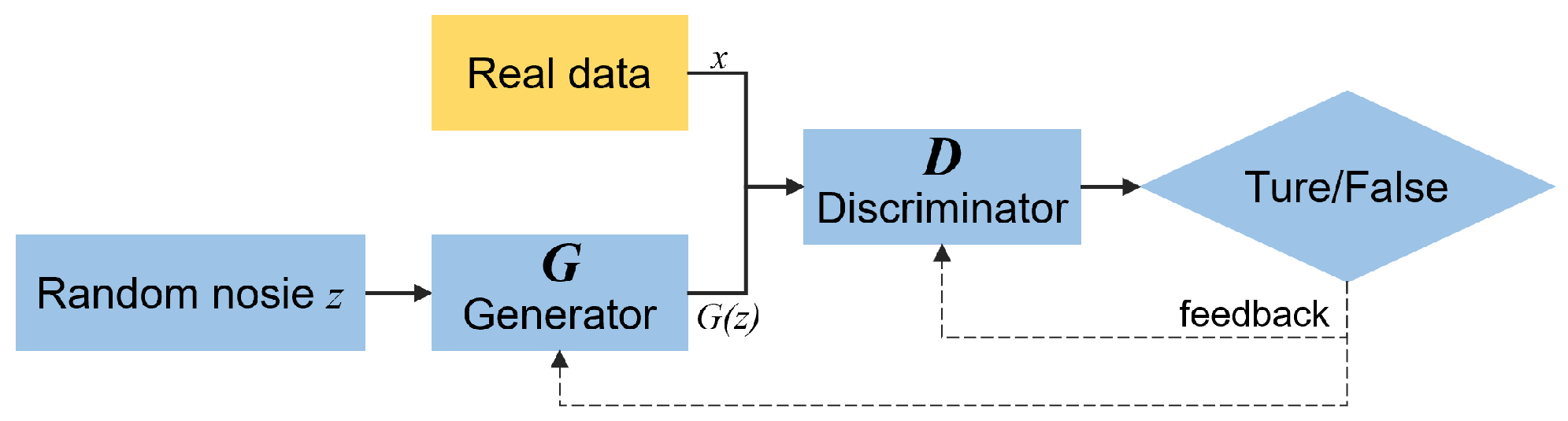
In 2014, Goodfellow et al. [29] proposed a GAN network based on zero-sum game theory. The network has two main components: the generator $\left(G\right)$ and the discriminator $\left(D\right)$. Figure 1 illustrates the network structure.

The principle is to pass a random noise signal z to G, so that G outputs the generated data $G\left(z\right)$ after learning the distribution of the real data x. $G\left(z\right)$ and x are fed simultaneously into the discriminator D, which determines whether $G\left(z\right)$ is a true probability value, with larger values representing a higher probability of being a true sample and vice versa. During training, G aims to create more convincing fake data to fool D, while D enhances its ability to tell real from fake data. This competition persists until G generates fake data almost identical to real data. The objective function is given as follows:

$$\underset{G}{min}\underset{D}{max}V(D,G)=E_{x\sim P_{\mathrm{data}\left(x\right)}}[logD\left(x\right)]+E_{z\sim P_z\left(z\right)}[log(1-D\left(G\left(z\right)\right))],$$

(1)

where $V(D,G)$ represents the discrepancy between generated and real samples, x and $G\left(z\right)$ denote the real sample input and generated output, respectively. $P_{data}$ and $P_z\left(Z\right)$ represent the real sample distribution and the noise distribution, including $D\left(x\right)$ and $D\left(G\right(z\left)\right)$ represent the probabilities of the real and generated data.

2.2. Deep Convolutional Generative Adversarial Network

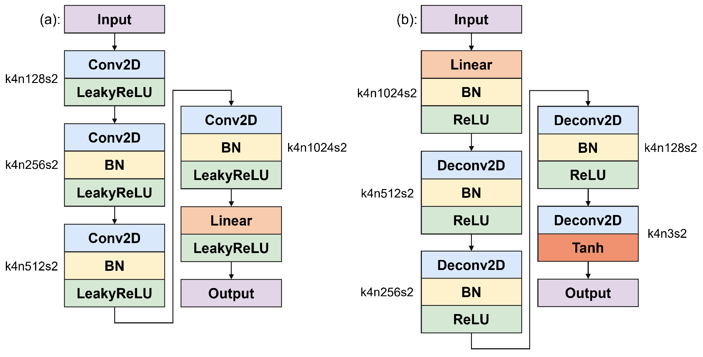
In 2016, Radford et al. [30] introduced CNN from supervised learning to GAN and proposed the DCGAN. The main improvement is that both the G and D networks of DCGAN discard the pooling layer of the CNN, with the D network retaining the CNN architecture and the G network replacing the convolutional layer with an inverse convolutional layer for up-sampling. Additionally, DCGAN introduces BN to improve the vanishing gradient problem and employs different activation functions: The generator applies ReLU activation for all layers except the output, which uses Tanh, while the discriminator applies Leaky ReLU for all layers to enhance the model’s expressiveness. Figure 2 illustrates the DCGAN architecture.

2.3. Minibatch Discrimination

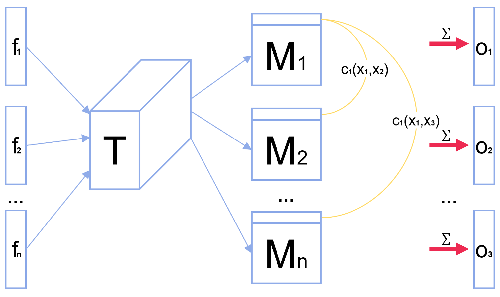
A major cause of DCGAN failure is mode collapse. This occurs because DCGAN lacks a mechanism to ensure that the generator produces diverse outputs. As mode collapse is imminent, the gradients of many similar points in the discriminator will point in a similar direction. To prevent this problem, it is crucial for the discriminator to combine multiple sample points at the same time during the training process, and to compute the differences between the features of the samples of the same batch to be used as additional inputs for the next layer [31]. This approach enables the rapid generation of samples that exhibit significant visual differences. The procedure is as follows: For each batch, there are n samples, where the vector corresponding to sample $x_i$ is $f\left(x_i\right)\in {\mathbb{R}}^A$, multiply $f\left(x_i\right)$ by a tensor $T\in {\mathbb{R}}^{A\times B\times C}$ to obtain a matrix $M_i\in {\mathbb{R}}^{B\times C}$. Finally, the $L_1$ distance is computed between the corresponding rows of each sample in $M_i$:

$$c_b\left(x_i,x_j\right)=exp\left(-{∥M_{i,b}-M_{j,b}∥}_{L_1}\right)\in \mathbb{R},$$

(2)

for sample $x_i$, the output $o\left(x_i\right)$ of this minibatch layer is the sum of $c_b(x_i,x_j)$ over the remaining samples:

$$o{\left(x_i\right)}_b=\sum _{j=1}^n{c}_b\left(x_i,x_j\right)\in \mathbb{R},$$

(3)

$$o\left(x_i\right)=\left[{o\left(x_i\right)}_1,{o\left(x_i\right)}_2,\dots ,{o\left(x_i\right)}_B\right]\in {\mathbb{R}}^B,$$

(4)

$$o\left(X\right)\in {\mathbb{R}}^{n\times B}.$$

(5)

Figure 3 illustrates the network structure of MD network.

2.4. Self-Attention Mechanism

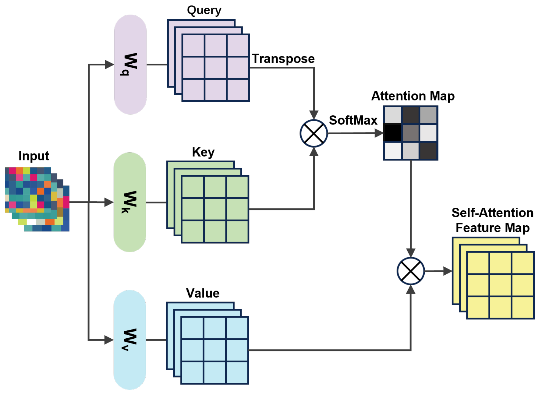
Conventional DCGAN typically uses convolutional operations to process images, which can only deal with local neighborhood information, making it difficult to establish long-range dependencies in images and generating high-resolution details with only fixed spatially localized points in low-resolution images. In contrast, SAM preserves the global integrity of the input sequences and effectively captures long-range dependencies across different locations [32]. Its introduction into DCGAN can generate more globally consistent feature representations, thus improving the performance of the generative network. Figure 4 illustrates the structure of the SAM module.

SA decomposes the input into three branches, query (Q), key (K), and value (V):

$$Q_i=W_q{x}_i,$$

(6)

$$K_i=W_k{x}_i,$$

(7)

$$V_i=W_v{x}_i.$$

(8)

where $W_q$, $W_k$, $W_v$ are the weighting matrices to be learned; $Q_i$, $K_i$, and $V_i$ denote the spaces obtained by multiplying image features with the corresponding weights. $Q_i$ is transposed and multiplied with $K_i$ to obtain $S_{ij}$, which is then normalized using the Softmax function to obtain the attention graph. The formula is as follows:

$$S_{ij}=Q_i^T{K}_j,$$

(9)

$${\rho }_{ij}={\displaystyle \frac{exp\left(S_{ij}\right)}{{\sum }_{i=1}^{N}exp\left(S_{ij}\right)}}.$$

(10)

where ${\rho }_{ij}$ denotes the degree of attention of the model to the position j at the position i. The resulting attention map ${\rho }_{ij}$ is multiplied by $V_i$ to obtain the self-attention feature map. The formula is as follows:

$$o_i=\sum _{i=1}^N{\rho }_{ij}{V}_i.$$

(11)

The final output $y_j$ represents a weighted representation of each input location in context, containing the information fusion and contextual relationships with other locations. The self-attentive feature map is multiplied by a scalar parameter, then weighted and summed with the original input to serve as input for the next hidden layer. The formula is as follows:

$$y_j=\gamma o_i+x_i.$$

(12)

where $\gamma$ is a learnable scalar that is introduced to progressively assign weights to long-range information.

2.5. Spectral Normalization

One challenge in training GAN is that as the discriminator becomes better trained, the gradients tend to vanish. The weight normalization approach used in SN can make the discriminator D realize Lipschitz constraint, meet the constraint condition of maximum slope of 1, limit the severity of function changes, and thus make the model more stable [33]. The formula is as follows:

$${\overline{W}}_{SN}\left(W\right)={\displaystyle \frac{W}{\sigma \left(W\right)}}.$$

(13)

where $\sigma \left(W\right)$ is the spectral norm of weighting matrix W. $SN$ of the weight matrix W of each convolutional layer in the discriminator D ensures that the model’s network parameter W varies smoothly during the optimization process and reduces the risk of gradient vanishing and gradient explosion, thus improving network stability.

2.6. Two-Timescale Update Rule

In the standard GAN framework, the discriminator and generator are co-optimized using the same learning rate. However, this approach can lead to issues such as gradient vanishing, mode collapse, and non-convergence of the loss function. TTUR, proposed by Heusel et al. [34], based on stochastic approximation theory, addresses this problem by treating the parameter updates of the discriminator and generator as two coupled stochastic processes. The core idea is to set different learning rates for the two components to control their convergence rates. In this study, a smaller learning rate is applied to the discriminator to ensure stable updates, while a larger learning rate is used for the generator to enhance its responsiveness to the gradient feedback from the discriminator.

3. Method

The improved DCGAN Algorithm 1 flow is presented below.

Algorithm 1 Improved DCGAN Algorithm.

Require:  Training datasets $\mathcal{X}$, batch size m, noise dimension $z_{dim}$, total epochs E, generator G, discriminator D, optimizer ${\theta }_G,{\theta }_D$ Ensure:  Trained generator $G^{*}$ and discriminator $D^{*}$    1: Initialize weights for G and D    2: Set Adam optimizer ${\theta }_G$ for G with initial learning rate ${\alpha }_G$    3: Set Adam optimizer ${\theta }_D$ for D with initial learning rate ${\alpha }_D$    4: Define label smoothing parameter $ϵ=0.1$    5: Define learning rate schedulers ${\mathcal{S}}_G,{\mathcal{S}}_D$    6: for epoch ← 1 to E do    7:     Shuffle training data and create mini-batches    8:     for each mini-batch $\mathbf{x}\in \mathcal{X}$ do    9:         Discriminator Training:  10:         Generate noise vectors ${\mathbf{z}}_1,{\mathbf{z}}_2\sim \mathcal{N}(0,1)$  11:         Generate fake images $\tilde{\mathbf{x}}\leftarrow G\left({\mathbf{z}}_1\right)$  12:         Compute real image loss:  13:         ${\mathbf{y}}_{real}\leftarrow (1-ϵ)·1+ϵ·0$                                                                                                                                                                                  ▹ Label smoothing  14:         ${\mathcal{L}}_{real}\leftarrow \mathrm{BCEWithLogitsLoss}(D\left(\mathbf{x}\right),{\mathbf{y}}_{real})$  15:         Compute fake image loss:  16:         ${\mathbf{y}}_{fake}\leftarrow (1-ϵ)·0+ϵ·1$                                                                                                                                                                                 ▹ Label smoothing  17:         ${\mathcal{L}}_{fake}\leftarrow \mathrm{BCEWithLogitsLoss}(D\left(\tilde{\mathbf{x}}\right),{\mathbf{y}}_{fake})$  18:         ${\mathcal{L}}_D\leftarrow ({\mathcal{L}}_{real}+{\mathcal{L}}_{fake})/2$  19:         Backpropagate ${\mathcal{L}}_D$ and update ${\theta }_D$  20:         Generator Training:  21:         Generate new noise ${\mathbf{z}}_2\sim \mathcal{N}(0,1)$  22:         Generate refined images ${\tilde{\mathbf{x}}}_{new}\leftarrow G\left({\mathbf{z}}_2\right)$  23:         Compute generator loss:  24:         ${\mathcal{L}}_G\leftarrow \mathrm{BCEWithLogitsLoss}(D\left({\tilde{\mathbf{x}}}_{new}\right),{\mathbf{y}}_{real})$  25:         Backpropagate ${\mathcal{L}}_G$ and update ${\theta }_G$  26:         Apply Improvements:  27:         Insert self-attention after deconv layers in G                                                                                                                                               ▹ Self-Attention  28:         Apply minibatch discrimination before D’s output                                                                                                                ▹ Minibatch Discrimination  29:         Update learning rate ${\alpha }_G\leftarrow {\mathcal{S}}_G\left(\mathrm{epoch}\right)$  30:         Update learning rate ${\alpha }_D\leftarrow {\mathcal{S}}_D\left(\mathrm{epoch}\right)$  31:    end for  32:    if epoch $mod$ save_interval $=0$ then  33:         Visualize intermediate generated samples  34:         Save model checkpoints $G_{\mathrm{epoch}}$ and $D_{\mathrm{epoch}}$  35:    end if  36: end for

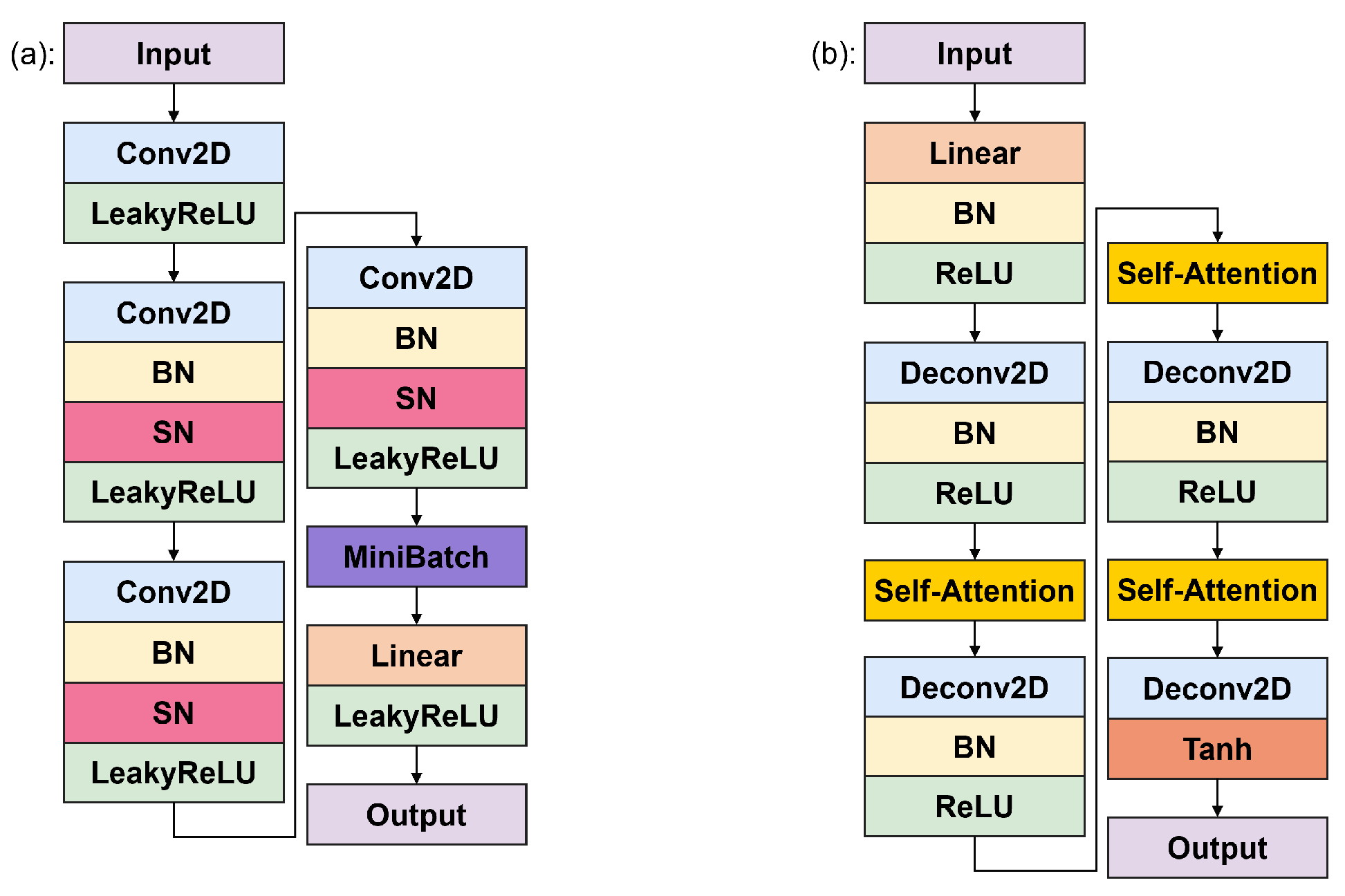
The structure of the improved DCGAN is depicted in Figure 5. Incorporating MD network after the discriminator’s final convolutional layer enhances its ability to differentiate between generated samples, mitigates mode collapse, and promotes the diversity of generated samples. Applying SN to each layer of convolution of the discriminator limits the number of spectral paradigms of the weight matrix, reduces the gradient explosion and vanishing problems, and makes the discriminator more accurate and stable in distinguishing between real and generated images. It is worth noting that citing SN does not eliminate the need for BN in the model. SN affects the weight of each layer, while BN affects the activation of each layer. Introducing SAM into the generator helps it better understand the global–local relationship, captures long-range dependencies between different regions in the image, and enables the generator to more accurately learn the structure and content of the image, thus generating more realistic images.

3.1. Discriminator Networks

The detailed structure of the improved discriminator network is presented in

Table 1. Discriminator details.

Convolutional Layer Input	Convolutional Layer Operation	Convolutional Layer Output
$64\times 64\times 3$	Conv2d: (k4, n128, s2) BN SN Leaky ReLU (negative slope = 0.2)	$32\times 32\times 128$
$32\times 32\times 128$	Conv2d: (k4, n256, s2) BN SN Leaky ReLU (negative slope = 0.2)	$16\times 16\times 256$
$16\times 16\times 256$	Conv2d: (k4, n512, s2) BN SN Leaky ReLU (negative slope = 0.2)	$8\times 8\times 512$
$8\times 8\times 512$	Conv2d: (k4, n512, s2) BN SN Leaky ReLU (negative slope = 0.2)	$4\times 4\times 1024$
$4\times 4\times 1024$	MD	$1\times$32,768
$1\times$32,768	Linear	$1\times 1$

, with its number of convolutional layers matching that of the original DCGAN.

The network takes a $64\times 64\times 3$ RGB image as input, with a $4\times 4$ convolution kernel, a stride of 2, and a Leaky ReLU activation function with a slope of 0.2. Both BN and SN are introduced in the convolutional layer to make the training performance more stable. After four layers of convolution the (4, 4, 1024) tensor is obtained, then MD is introduced after the last layer of convolution by which the tensor obtained is computed and spliced with the input information, this tensor represents the exponential sum of the differences between each sample in the current batch and the other samples, and this tensor is expanded in the last dimension to match the shape of the input information, and the final result is a 32,768 dimensional vector.

3.2. Generator Networks

Table 2. Generator details.

Convolutional Layer Input	Convolutional Layer Operation	Convolutional Layer Output
100	Linear	$4\times 4\times 1024$
$4\times 4\times 1024$	Deconv2d: (k4, n512, s2)BN ReLU	$8\times 8\times 512$
$8\times 8\times 512$	SAM	$8\times 8\times 512$
$8\times 8\times 512$	Deconv2d: (k4, n256, s2)BN ReLU	$16\times 16\times 256$
$16\times 16\times 256$	SAM	$16\times 16\times 256$
$16\times 16\times 256$	Deconv2d: (k4, n128, s2)BN ReLU	$32\times 32\times 128$
$32\times 32\times 128$	SAM	$32\times 32\times 128$
$32\times 32\times 128$	Deconv2d: (k4, n64, s2)BN Tanh	$64\times 64\times 3$

presents the detailed architecture of the improved generator network, which consists of a total of four transposed convolutional layers and three SA modules.

The generator first converts the 100-dimensional noise signal into a (4, 4, 1024) three-dimensional tensor by means of a fully connected layer, and then performs layer-by-layer convolution, with each layer of convolution corresponding to the dimensions in the discriminator, and adds SAM after the each convolutional layers, and ultimately outputs a $64\times 64\times 3$ image. A Tanh function is applied in the output layer, while ReLU activation functions are used in the other convolutional layers. The Tanh function compresses output values into the range (−1, 1), aligning with the standard format for image data preprocessing—this allows the pixel values of the generated image to be easily mapped to the desired range via a simple linear transformation. When incorporating the SAM in the generator, the extracted feature maps need to be converted into Query, Key and Value representations after three convolutional layers with convolutional kernel of 1, respectively. Key and Query are used together to compute the attention weights, and Value is weighted and combined based on the computed attention weights to obtain a richer and more expressive feature representation.

4. Result

The experimental equipment used in this paper is Intel (R) Core (TM) i9-13950HX 2.20 GHz (Intel Corporation, Santa Clara, CA, USA), NVIDIA RTX 3500Ada Generation Laptop GPU (NVIDIA Corporation, Santa Clara, CA, USA), and a PyTorch (Python 3.9, CUDA 12.1, TorchVision 0.17.1, TorchAudio 2.2.1) environment. Since the generator’s performance is generally weaker than the discriminator’s, this imbalance may lead to mode collapse in DCGAN during the early training phase. Therefore, the single learning rate of DCGAN was replaced with the TTUR, which assigns separate learning rates to the discriminator and generator to ensure early training stability. The experiments used the Adam optimizer, with the generator’s learning rate set to 2 $\times {10}^{-4}$ and the discriminator’s rate set to 3 $\times {10}^{-5}$ for a total of 3000 training rounds.

Table 3. Complexity comparison.

Parameter Type	DCGAN	Improved DCGAN
D: Total Parameters (M)	11.04	11.05
D: Forward/Backward Pass Size (MB)	4.63	5.88
G: Total Parameters (M)	12.68	13.11
G: Forward/Backward Pass Size (MB)	5.72	18.19

presents a comparison of the model’s complexity before and after the improvement. The results show that the total number of parameters in the generator and discriminator has increased only slightly, suggesting that the optimization of the model structure has not introduced significant parameter redundancy. While the memory footprint for the generator’s forward/backward propagation has increased, this trade-off is essential for enhancing the quality of generated outputs.

4.1. Preprocessing of Data Sets

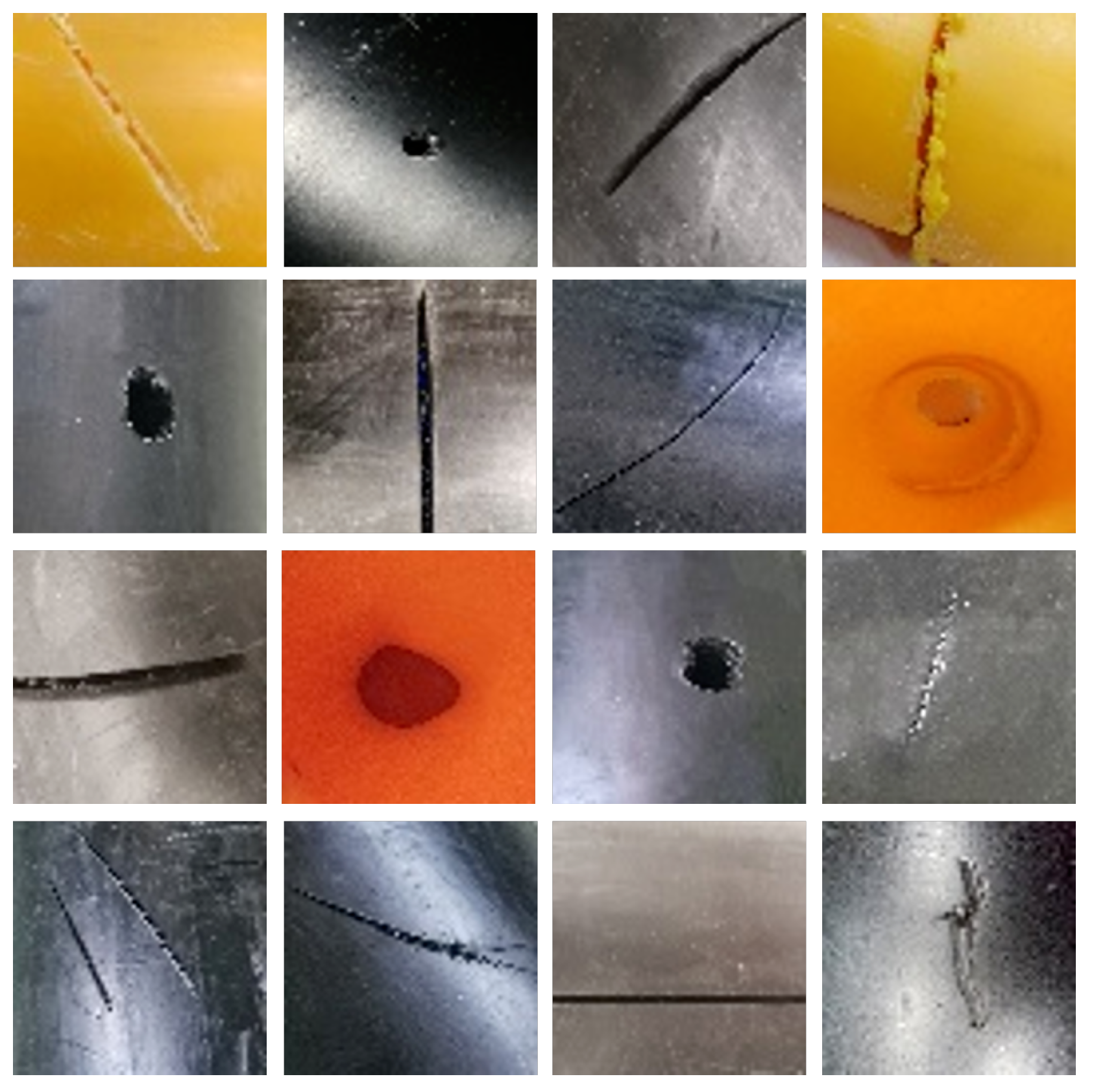
The experiment in this study was conducted using a defect datasets of gas PE pipelines, consisting of 150 defects categorized as cracks, fractures, and holes. During the training of a GAN, a small datasets can lead to overfitting, resulting in generated images that lack diversity and realism. In order to avoid this problem, the datasets is first pre-enhanced. Specifically, geometric transformations such as mirroring, rotation, and translation were applied, along with noise addition, expanding the datasets to 1000 defective images. For the sake of facilitating the comparison of the results, the sample size of the datasets was uniformly processed to $64\times 64$ size, and Figure 6 shows some of the images of the pipeline defect datasets.

4.2. Visualize Comparisons

Generate Image Comparisons

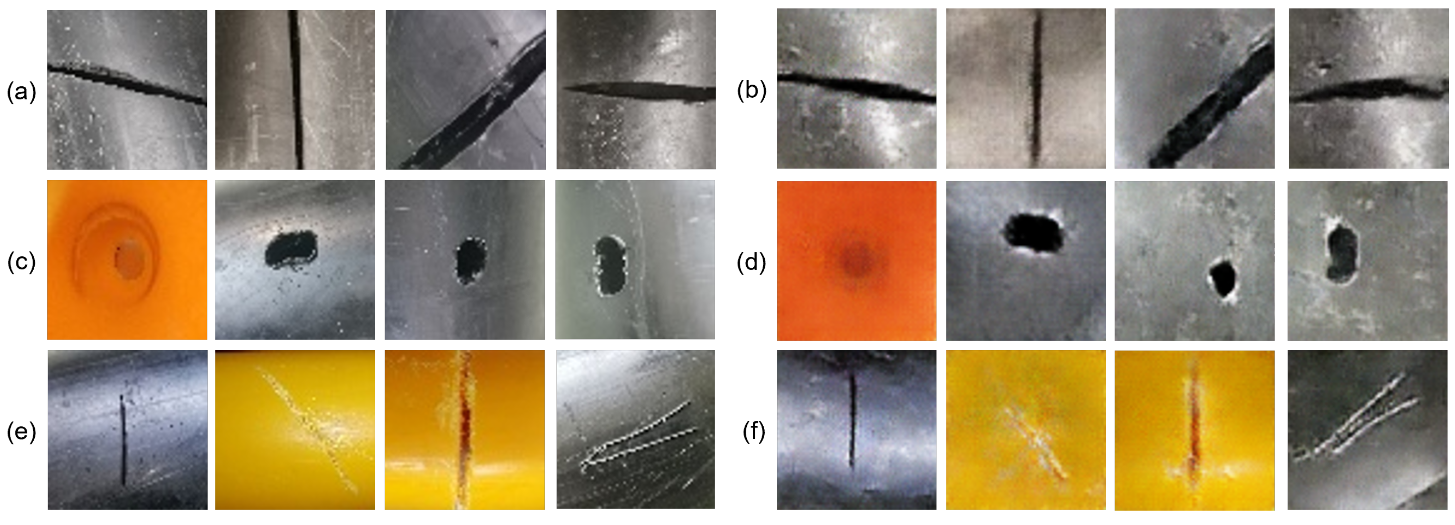
Firstly, the improved DCGAN generation results are compared with the real defective images, as illustrated in Figure 7.

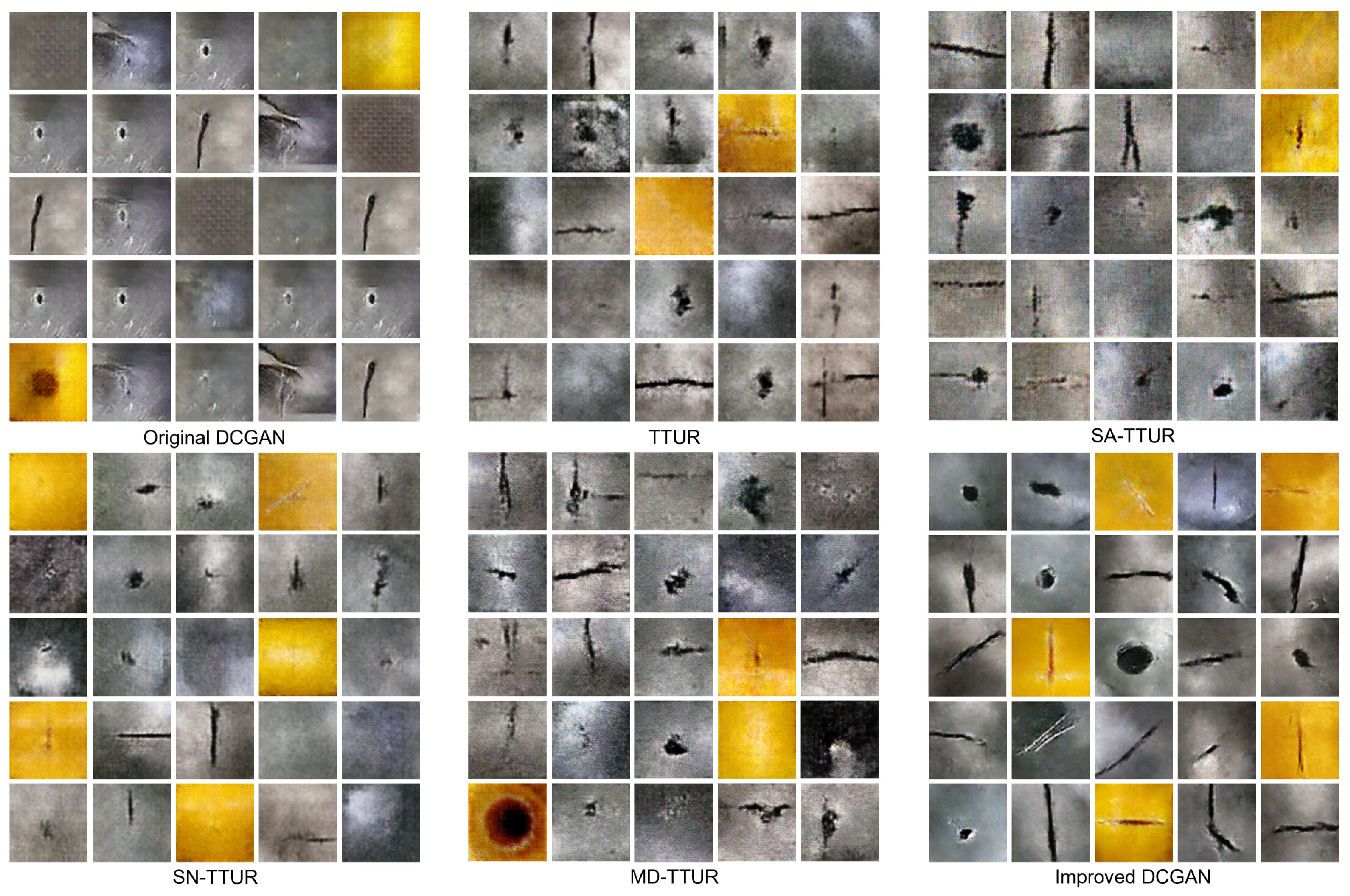
It can be seen that the image generated by the improved DCGAN has clear contours and can fit the real image with superior generation quality. Figure 8 illustrates the images generated by each sub-model and the improved DCGAN to further validate the effectiveness of the algorithm improvements.

The comparison reveals that the original DCGAN suffered from mode collapse and generated images with low clarity. In contrast, the TTUR model demonstrated improved stability compared to the single learning rate used in the original DCGAN, effectively mitigating the mode collapse issue. Building on this, the SA-TTUR and SN-TTUR models further enhanced generator performance, but there is still some noise. MD-TTUR improves in generating image diversity compared to other sub-models. While the improved DCGAN model generates images that are more compatible with the features of real images, the image clarity is close to that of real images and generates shapes that are not present in the original images, the diversity and model training stability are significantly improved.

4.3. Convergence Analysis

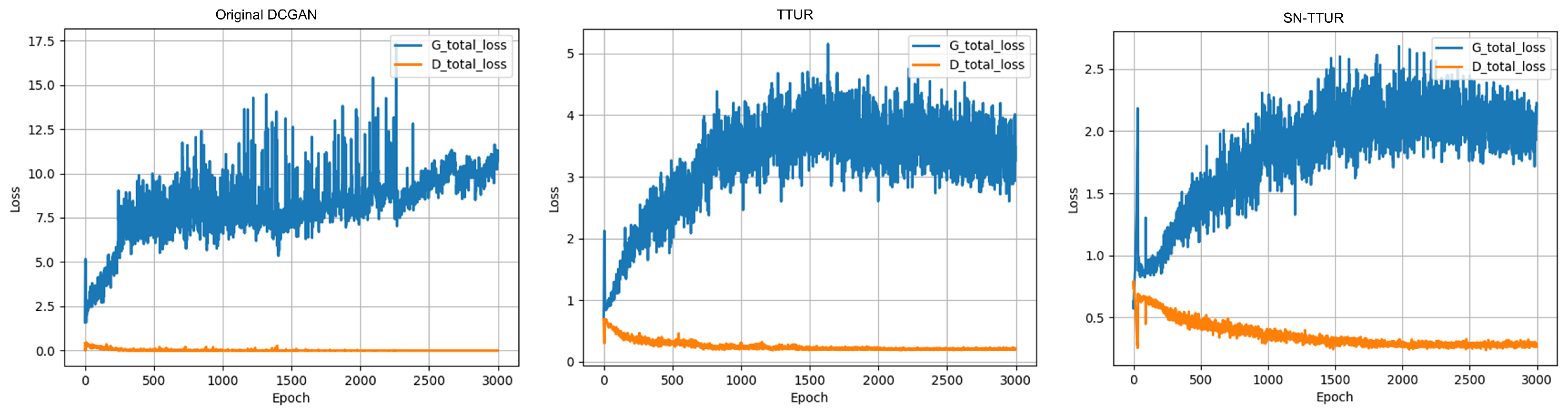
The ability of TTUR and SN modules to enhance training stability requires further validation. To assess the effectiveness of these improvements, we compared the generator and discriminator losses of the Original DCGAN, TTUR, and SN-TTUR. The resulting training losses are presented in Figure 9. The figure demonstrates that with an increasing number of training epochs, the generator loss in the Original DCGAN continues to rise, while the discriminator loss approaches zero, which indicates that the generator’s performance is weaker than that of the discriminator. In contrast, with TTUR, the generator loss exhibits a smoother decrease, and is significantly lower than that of the Original DCGAN. The SN-TTUR generator loss values are further reduced, and its fluctuation stabilizes, indicating that combining these two modules enhances the training stability of the DCGAN model. With the simultaneous application yielding the most favorable results.

4.4. Quantitative Evaluation of Generated Images

4.4.1. Image Evaluation Indicators

Since subjective qualitative methods alone are sometimes insufficient to assess image quality, quantitative evaluation methods are also needed for a more comprehensive analysis. Firstly, two image evaluation metrics, FID and SSIM compare the generated and real images based on defect types, and the average value is then obtained to measure the clarity and variety of the generated images. FID evaluates image quality, diversity, and is often used to compare the performance of GAN and other generation models. It evaluates the quality of an image by measuring the feature difference between the generated and real samples; a lower FID score indicates better image quality and diversity, with the ideal case being 0. SSIM is a metric that compares the brightness, contrast, and structure between two images. Unlike traditional disparity measures, SSIM aligns more closely with human visual perception and is closer to actual perception. SSIM has a value between 0 and 1. Values closer to 1 indicate better generated image quality.

Table 4. FID and SSIM scores of the generated images.

Evaluation Scores	DCGAN	DCGAN-TTUR	SA-TTUR	SN-TTUR	MiniBatch-TTUR	Improved DCGAN
FID	234.868	228.962	198.519	219.143	205.735	184.267
SSIM	0.325	0.406	0.414	0.478	0.370	0.601

presents the FID and SSIM evaluation scores for each model. The results in Table 4 indicate that the improved DCGAN model achieves superior performance across both metrics.

The scores of SA-TTUR, SN-TTUR and MD-TTUR in FID and SSIM have advantages and disadvantages, because FID can reflect the diversity of generated images to a certain extent, that is, SA-TTUR and MD-TTUR have better performance in generating image diversity. SN-TTUR produces better image quality. It also shows that the improved DCGAN model makes full use of the capabilities of each module to enhance the model performance.

4.4.2. Classified Evaluation Indicators

In addition to the image evaluation metrics, which is a quantitative evaluation method, classification index offers an alternative perspective to assess the enhancements introduced by the improved DCGAN model. The VGGNet, AlexNet and ResNet classifiers are used to train the three data augmentation methods (T1: traditional data augmentation, T2: improved DCGAN, T3: traditional data augmentation + improved DCGAN), respectively, and

Table 5. Classification Results.

Model	Data Augmentation Methods	Accuracy (%)	G-Mean (%)	F-Score (%)
VGGNet	T1	78.23	53.81	70.12
	T2	81.26	68.10	75.92
	T3	83.33	76.81	80.34
AlexNet	T1	72.90	55.62	66.86
	T2	76.99	68.40	72.41
	T3	83.08	74.19	78.15
ResNet	T1	71.14	66.25	68.80
	T2	74.19	67.89	70.94
	T3	76.82	73.63	74.53

presents the training results for the three classifiers.

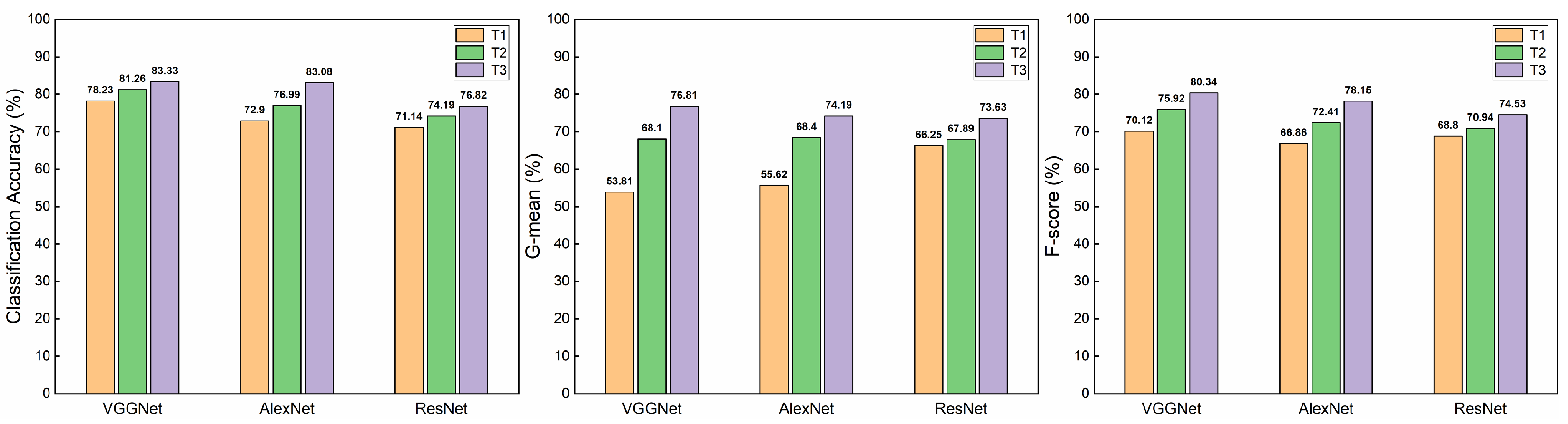
The T1 datasets exhibited the lowest performance, with accuracies of 78.23%, 72.90%, and 71.14% for the three classifiers. The corresponding G-mean values were 53.81%, 55.62%, and 66.25%, while the F-score were 70.12%, 66.86%, and 68.80%. In comparison, the T2 datasets showed improvements in accuracy by 3.03%, 4.09%, and 3.05% over T1. G-mean increased by 14.29%, 12.78%, and 1.64%, and F-score improved by 5.8%, 5.55%, and 2.14%. Notably, the T3 datasets achieved the highest accuracy across all three classifiers, with increases of 2.07%, 6.09%, and 2.63% over T2, reaching 83.33%, 83.08%, and 76.82%, respectively. G-mean improved by 8.71%, 5.79%, and 5.74% over T2, reaching 76.81%, 74.19%, and 73.63%, respectively. F-score increased by 4.42%, 5.74%, and 3.59% over T2, reaching 80.34%, 78.15%, and 74.53%, respectively. Bar charts are plotted according to Table 5 for a more intuitive view of the performance of the improved DCGAN, as shown in Figure 10.

As shown in the figure, after data augmentation using the improved DCGAN, all metrics significantly improved, with T3 achieving the highest accuracy. This demonstrates that the hybrid datasets substantially enhances classifier performance, further validating the effectiveness of the generated gas PE pipe defective images.

4.4.3. Effect of the Number of Expanded Images on Accuracy

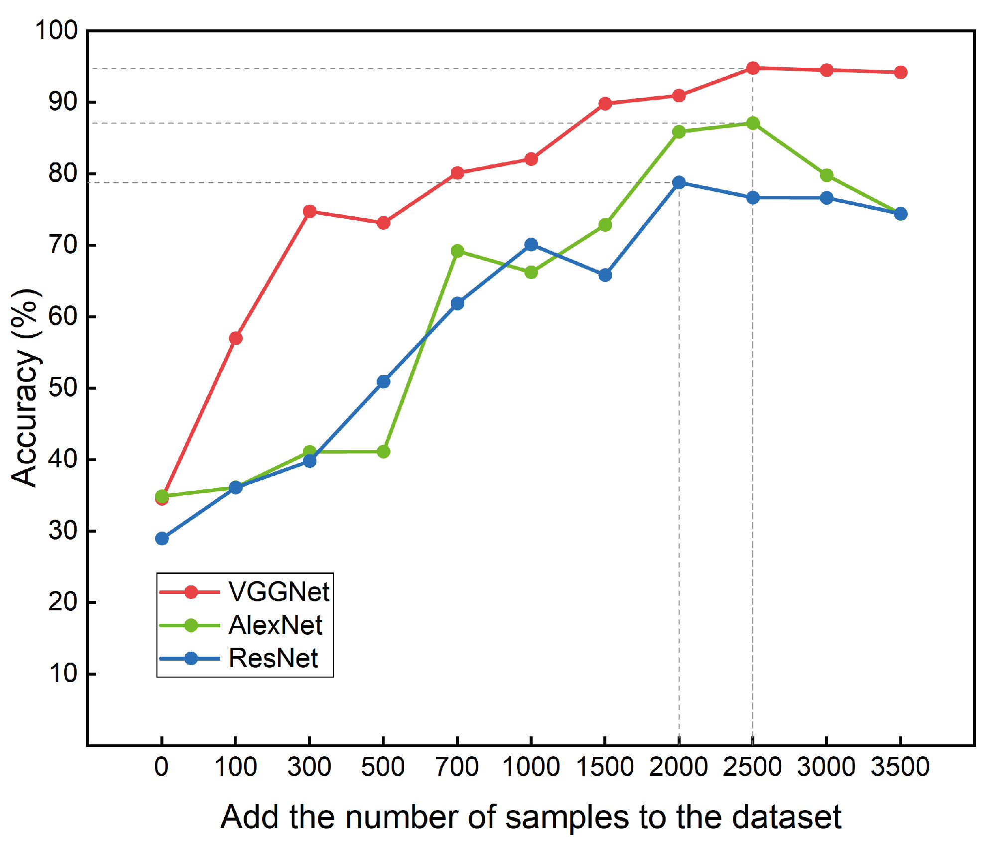
In order to determine the impact of the number of expanded images on the classification accuracy, T3 data augmentation method, which has the best performance in Section 4.4.2, is adopted to successively expand the images of the original datasets to test the accuracy. That is, on the basis of the original images, the expanded images and generated images by traditional data augmentation methods are added at the same time. The number of augmented images was gradually increased in steps of 100, 300, 500, 700, 1000, 1500, 2000, 2500, 3000, and 3500 to determine the optimal augmentation level. Figure 11 shows the experimental results.

With the gradual increase in the expanded images, the accuracy of each classifier was enhanced with different extents. The accuracy of ResNet reached its highest value of 78.79% when the number of expanded images was 2000. When 2500 images were expanded, VGGNet and AlexNet achieved accuracies of 94.79% and 87.1%, respectively. And as the number of expansions continued to increase, the accuracy of each classifier did not improve further, but decreased. This decline could be attributed to the limited size of the original datasets, which constrained the diversity of features learnable by the improved DCGAN. As the amount of generated data in the classifier increases, overfitting occurs, resulting in a decline in accuracy.

5. Conclusions

Due to the limited number of defective images within gas polyethylene pipes, this study proposes an improved DCGAN. The key contributions are as follows:

• Network Architecture Optimization: By combining Minibatch Discrimination, Spectral Normalization, and the DCGAN model, the network architecture is refined using the Two-Timescale Update Rule. This modification addresses the limitations of the original DCGAN, such as its tendency for pattern collapse, enhances the quality and diversity of generated samples, and mitigates the issue of unstable training caused by the generator being weaker than the discriminator. Additionally, the introduction of the Self-Attention Mechanism further refines the detailed features of the generated images.
• Generation Quality Assessment: The similarity between the generated images from the improved DCGAN model and the real images is first validated through visual comparison. The effects of different sub-models are also compared. Experimental results show that, after introducing TTUR, the generator loss amplitude is reduced by approximately 66%, while the maximum loss value of SN-TTUR decreases by around 83.33% compared to the original DCGAN. Regarding quantitative image evaluation metrics, the FID of defective images generated by the improved model is reduced by 21.5%, and the SSIM score increases by 45.9% compared to the original DCGAN. In classification validation experiments, the accuracy of VGGNet, AeNetx, and ResNet, based on the hybrid datasets, reaches 83.33%, 83.08%, and 76.82%, respectively, improving by 5.1%, 10.18%, and 5.68% compared to traditional data augmentation methods. The G-mean improves by 23%, 18.57%, and 7.38%, while the F-score improves by 10.22%, 11.29%, and 5.73%, respectively.
• The relationship between the generated defective image quantity and classification accuracy was explored. Classifier performance improved universally when incorporating these generated images.

This study addresses the issues of data scarcity and uneven distribution through an improved DCGAN, but in the future, there is still a need to enrich and diversify the datasets to further supplement the defective samples under actual working conditions to better cope with the complexity of real-world applications. These samples should cover a wide range of factors such as different environmental conditions, pipeline aging and human interference, to ensure that the inspection system can operate effectively in a variety of complex and dynamic real-world scenarios. The robustness and generalization ability of the model can be further improved by introducing more actual working condition data, thus enhancing the accuracy and reliability of defect detection.

References

- Palma, A.; Paltrinieri, A.; Goodell, J.W.; Oriani, M.E. The black box of natural gas market: Past, present, and future. Int. Rev. Financ. Anal. 2024, 94, 103260. [Google Scholar] [CrossRef]
- Li, J.; She, Y.; Gao, Y.; Li, M.; Shi, Y. Natural gas industry in China: Development situation and prospect. Nat. Gas Ind. B 2020, 7, 604–613. [Google Scholar] [CrossRef]
- Li, N.; Wang, J.; Liu, R.; Zhong, Y.; Shi, Y. What is the short-term outlook for the EU’s natural gas demand? Individual differences and general trends based on monthly forecasts. Environ. Sci. Pollut. Res. 2022, 94, 78069–78091. [Google Scholar] [CrossRef]
- Guan, Y. The application practice of PE gas pipeline in municipal gas engineering. Chem. Eng. Manag. 2018, 21, 102. [Google Scholar]
- Nasiri, S.; Khosravani, M.R. Failure and fracture in polyethylene pipes: Overview, prediction methods, and challenges. Eng. Fail. Anal. 2023, 152, 107496. [Google Scholar] [CrossRef]
- Wang, H.; Shah, J.; Hawwat, S.E.; Huang, Q.; Khatami, A. A comprehensive review of polyethylene pipes: Failure mechanisms, performance models, inspection methods, and repair solutions. J. Pipeline Sci. Eng. 2024, 4, 100174. [Google Scholar] [CrossRef]
- Mohsin, R.; Majid, Z.A. Erosive Failure of Natural Gas Pipes. J. Pipeline Syst. Eng. Pract. 2014, 5, 04014005. [Google Scholar] [CrossRef]
- Tutunchi, A.; Eskandarzade, M.; Aghamohammadi, R.; Masalehdan, T.; Osouli-Bostanabad, K. Risk assessment of electrofusion joints in commissioning of polyethylene natural gas networks. J. Int. J. Press. Vessel. Pip. 2022, 196, 104627. [Google Scholar] [CrossRef]
- Cai, Q.; Huang, B.; Han, P.; Guo, X. Research progress on main defects and non-destructive testing technology of hot melt joints of polyethylene gas pipelines. Chem. Eng. Equip. 2020, 6, 221–223. [Google Scholar]
- Shi, J.; Fen, Y.; Tao, Y.; Zheng, J.; Liang, L. Advances in technical standards for non-destructive testing of polyethylene pipes. Press Vessel Technol. 2021, 38, 66–75. [Google Scholar]
- Tang, Y.; Xia, X.; Zhao, J.; Han, Z.; Zou, J. Pipe wall thickness measurement method based on mobile X-ray detection system. Pipeline Tech. Equip. 2022, 2, 35–41. [Google Scholar]
- Kafieh, R.; Lotfi, T.; Amirfattahi, R. Automatic detection of defects on polyethylene pipe welding using thermal infrared imaging. Infrared. Phys. Technol. 2011, 54, 317–325. [Google Scholar] [CrossRef]
- Gao, B.; Zhao, H.; Miao, X. A novel multi-model cascade framework for pipeline defects detection based on machine vision. Measurement 2023, 220, 113374. [Google Scholar] [CrossRef]
- Zamora, J.D.; Tang, C. Visual data restoration for pipeline inspection robots by compressed sensing. In Proceedings of the 2024 8th International Conference on Robotics, Control and Automation (ICRCA), Shanghai, China, 12–14 January 2024; Volume 8. [Google Scholar]
- Xie, Q.; Dai, Z.; Hovy, E.; Luong, T.; Le, Q. Unsupervised data augmentation for consistency training. Adv. Neural. Inf. Process Syst. 2020, 33, 6256–6268. [Google Scholar]
- Kang, L.; Su, Z. A Review of the Principles and Development of Image Data Augmentation Techniques. Inf. Technol. 2024, 9, 176–185. [Google Scholar]
- Setiawan, A.; Yudistira, N.; Wihandika, R.C. Large scale pest classification using efficient Convolutional Neural Network with augmentation and regularizers. Comput. Electron. Agric. 2022, 200, 107204. [Google Scholar] [CrossRef]
- Mangla, P.; Singh, V.; Havaldar, S.; Balasubramanian, V. On the benefits of defining vicinal distributions in latent space. Pattern Recognit. Lett. 2021, 152, 382–390. [Google Scholar] [CrossRef]
- Pandey, A.; Pati, U.C. Image mosaicing: A deeper insight. Image Vis. Comput. 2019, 89, 236–257. [Google Scholar] [CrossRef]
- Guan, H.; Zhao, L.; Dong, X.; Chen, C. Extended natural neighborhood for SMOTE and its variants in imbalanced classification. Eng. Appl. Artif. Intell. 2023, 124, 106570. [Google Scholar] [CrossRef]
- Cubuk, E.D.; Zoph, B.; Mane, D.; Vasudevan, V.; Le, Q.V. Autoaugment: Learning augmentation policies from data. arXiv 2018, arXiv:1805.09501. [Google Scholar]
- Aggarwal, A.; Mittal, M.; Battineni, G. Generative adversarial network: An overview of theory and applications. Int. J. Inf. Manag. Data Insights 2021, 1, 100004. [Google Scholar] [CrossRef]
- Dash, A.; Ye, J.; Wang, G. A review of generative adversarial networks (gans) and its applications in a wide variety of disciplines: From medical to remote sensing. IEEE Access 2024, 12, 18330–18357. [Google Scholar] [CrossRef]
- Tan, H.; Hu, Y.; Ma, B.; Yu, G.; Li, Y. An improved DCGAN model: Data augmentation of hyperspectral image for identification pesticide residues of Hami melon. Food Control 2024, 157, 110168. [Google Scholar] [CrossRef]
- Min, Y.; Li, J.; Wang, G. Image expansion method for rail surface defects based on improved DCGAN. China Railw. Soc. 2023, 45, 123–130. [Google Scholar]
- Dewi, C.; Chen, R.; Liu, Y.; Tai, S.; Shi, Y. Synthetic Data generation using DCGAN for improved traffic sign recognition. Neural. Comput. Appl. 2022, 34, 21465–21480. [Google Scholar] [CrossRef]
- Woldesellasse, H.; Tesfamariam, S. Data augmentation using conditional generative adversarial network (cGAN): Application for prediction of corrosion pit depth and testing using neural network. J. Pipeline Sci. Eng. 2023, 3, 100091. [Google Scholar] [CrossRef]
- Popuri, A.; Miller, J. Generative adversarial networks in image generation and recognition. In Proceedings of the International Conference on Computational Science and Computational In telligence, Las Vegas, NV, USA, 13–15 December 2023; pp. 1294–1297. [Google Scholar]
- Goodfellow, I.; Pouget-Abadie, J.; Mirza, M.; Xu, B.; Warde-Farley, D.; Ozair, S.; Courville, A.; Bengio, Y. Generative adversarial nets. Adv. Neural. Inform. Process Syst. 2014, 27, 139–144. [Google Scholar]
- Radford, A. Unsupervised representation learning with deep convolutional generative adversarial networks. arXiv 2015, arXiv:1511.06434. [Google Scholar]
- Salimans, T.; Goodfellow, I.; Zaremba, W.; Cheung, V.; Radford, A.; Chen, X. Improved techniques for training gans. arXiv 2016, arXiv:1606.03498. [Google Scholar]
- Yildiz, E.; Yuksel, M.E.; Sevgen, S. A Single-Image GAN Model Using Self-Attention Mechanism and DenseNets. Neurocomputing 2024, 596, 127873. [Google Scholar] [CrossRef]
- Zhong, H.; Yu, S.; Trinh, H.; Lv, Y.; Shi, Y.; Yuan, R.; Wang, Y. Fine-tuning transfer learning based on DCGAN integrated with self-attention and spectral normalization for bearing fault diagnosis. Measurement 2023, 210, 112421. [Google Scholar] [CrossRef]
- Heusel, M.; Ramsauer, H.; Unterthiner, T. Gans trained by a two time-scale update rule converge to a local nash equilibrium. Adv. Neural. Inf. Process Syst. 2017, 30, 6629–6640. [Google Scholar]
Disclaimer/Publisher’s Note: The statements, opinions and data contained in all publications are solely those of the individual author(s) and contributor(s) and not of MDPI and/or the editor(s). MDPI and/or the editor(s) disclaim responsibility for any injury to people or property resulting from any ideas, methods, instructions or products referred to in the content. |
© 2025 by the authors. Licensee MDPI, Basel, Switzerland. This article is an open access article distributed under the terms and conditions of the Creative Commons Attribution (CC BY) license (https://creativecommons.org/licenses/by/4.0/).