
Coordinated Optimization of Feeder Flex-Route Transit Scheduling for Urban Rail Systems


Abstract
:1. Introduction
2. Literature Review
- (1)
- Joint Optimization of Path and Timetable—Unlike prior studies that optimize these components separately, this research integrates them to enhance coordination between flex-route transit and urban rail.
- (2)
- Passenger Demand and Transfer Behavior Analysis—The proposed model incorporates real-time demand data and passenger transfer patterns to enhance service reliability and efficiency.
- (3)
- A Dynamic Scheduling Framework—By developing a mixed-integer nonlinear programming (MINLP) model, this study introduces a more flexible and adaptive scheduling mechanism, allowing for real-time adjustments to improve system resilience.
- (4)
- Cost-Efficiency and Service Quality Trade-Off—The model considers both operator costs and passenger-centric factors (waiting times, transfer failures, travel delays) to find an optimal balance.
3. Mathematical Model
3.1. Model Assumptions
3.2. Notation
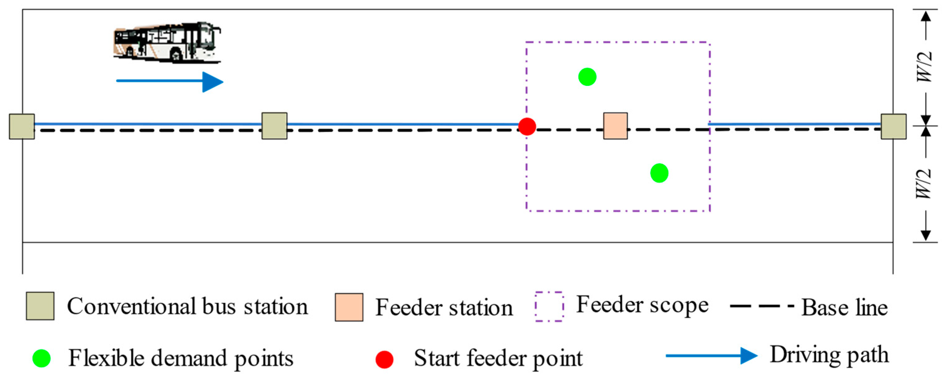
3.3. Flex-Route Transit Operation Organization Model
3.3.1. Objective Function
3.3.2. Constraint Condition
- (1)
- Vehicle operation constraints
- (2)
- Departure interval constraints
- (3)
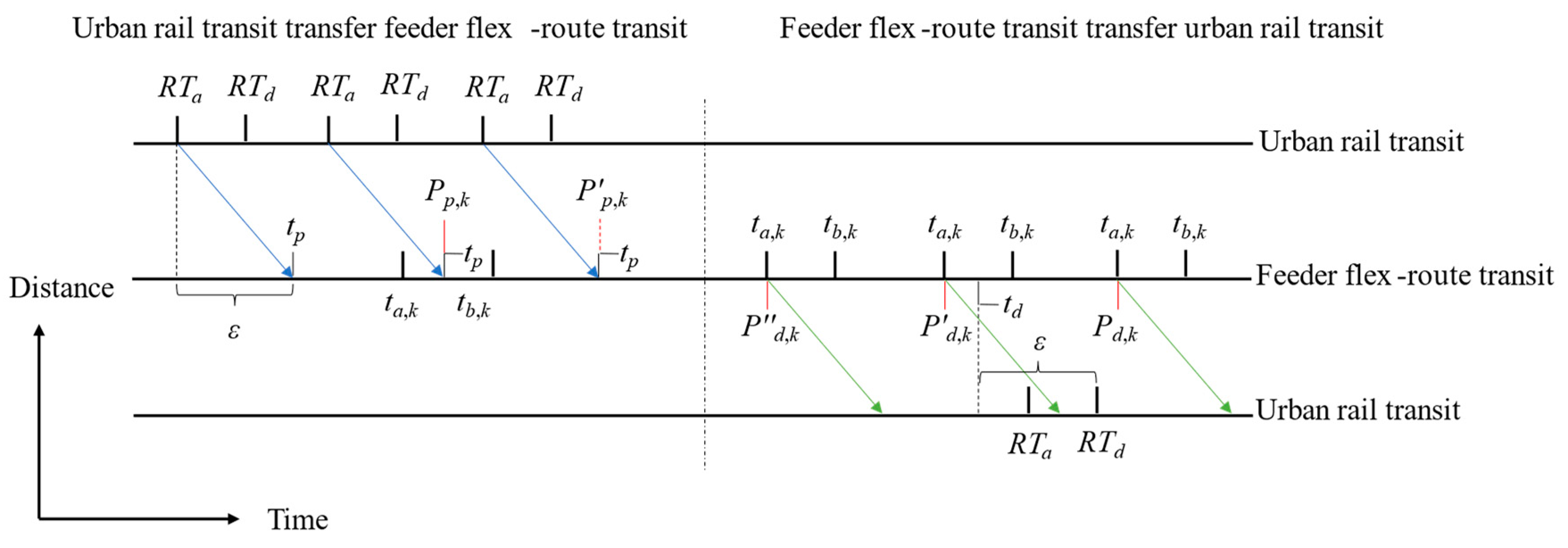
- Passenger transfer constraints
4. Solution Approach
4.1. Departure Interval Setting Stage
| Algorithm 1 Departure interval setting algorithm | |||
| Input: | Lower limit of departure interval Hmin, upper limit of departure interval Hmax, departure interval Hν, where: Hν = Hmin, …, Hmax, ν = 1, 2, …, n | ||
| Output: | Optimal departure interval H*, Optimal system cost U*(H*) | ||
| Step 0 | Take the initial departure interval H1 = Hmin, let the optimal departure interval H* = H1, calculate the current system cost U(H1), let the optimal system cost U*(H*) = U(H1); | ||
| Loop: | While ν < n | ||
| Step 1 | Based on the current departure interval, obtain a new vehicle departure interval Hν + 1,and judge the constraint condition, if Hν+1 does not satisfy the constraint condition, repeat Step 1; | ||
| Step 2 | Calculate the system cost U(Hν+1) under departure interval Hν+1, if U(Hν+1) < U*(H*), accept Hν+1 as the new optimal departure interval, H* = Hν+1, Otherwise, retain the original optimal departure interval H*; | ||
| Step 3 | If termination condition Hn = Hmax is satisfied, then output optimal departure interval H* and optimal system cost U*(H*), termination routine, Otherwise, repeat Step 1. | ||
4.2. Shift Setting Stage
| Algorithm 2 Shift setting algorithm | |||
| Input: | Population size, crossover probability, mutation probability, maximum number of iterations Imax | ||
| Output: | Optimal solution u, Optimal system cost U | ||
| Step 0 | Input feeder flex-route transit operation parameters, set population size, crossover probability, mutation probability, maximum number of iterations Imax, initialize the number of population iterations In = 0; | ||
| Loop: | While In < Imax | ||
| Step 1 | Encoding: chromosome adopts a matrix composed of 0–1 variables to reflect the two-dimensional relationship between passenger allocation and shift setting. Due to the phenomenon of rejection of passengers in flex-route transit, not all passengers can be served, so it is necessary to assume that there is a new virtual shift on the basis of all feeder shifts to store rejected passengers; | ||
| Step 2 | Fitness function: when the feeder flex-route transit completes a complete shift setting in the operation cycle, the fitness corresponding to the chromosome is calculated; | ||
| Step 3 | Chromosome update: (1) after the assignment and setting of each passenger and shift are completed, the system will reject the travel requirements of some passengers due to relevant constraints, feed back the information of the rejected passengers to the chromosome, and change the corresponding genes to achieve chromosome update; (2) if the current chromosome meets the constraints, but the quality is not high, it is easy to cause premature convergence. It is necessary to try to rearrange the rejected passengers back to the flex-route transit to improve the quality of the chromosome and jump out of the local optimum; | ||
| Step 4 | Selection: elite retention strategy and tournament method; | ||
| Step 5 | Crossing: select a single-point crossing method, arbitrarily select the position of the crossing point, use the crossing point as the boundary point, and recombine the two chromosomes; | ||
| Step 6 | Mutation: using a single point mutation method, when a chromosome undergoes mutation, randomly select the location where the gene will mutate, and passengers at that location will switch to the corresponding service shift; | ||
| Step 7 | Update population fitness, calculate the objective function values of offspring, update and record the optimal solution of the population; | ||
| Step 8 | Iteration count update, In = In + 1; | ||
| Step 9 | Algorithm termination conditions: In ≥ Imax. | ||
5. Result Analysis
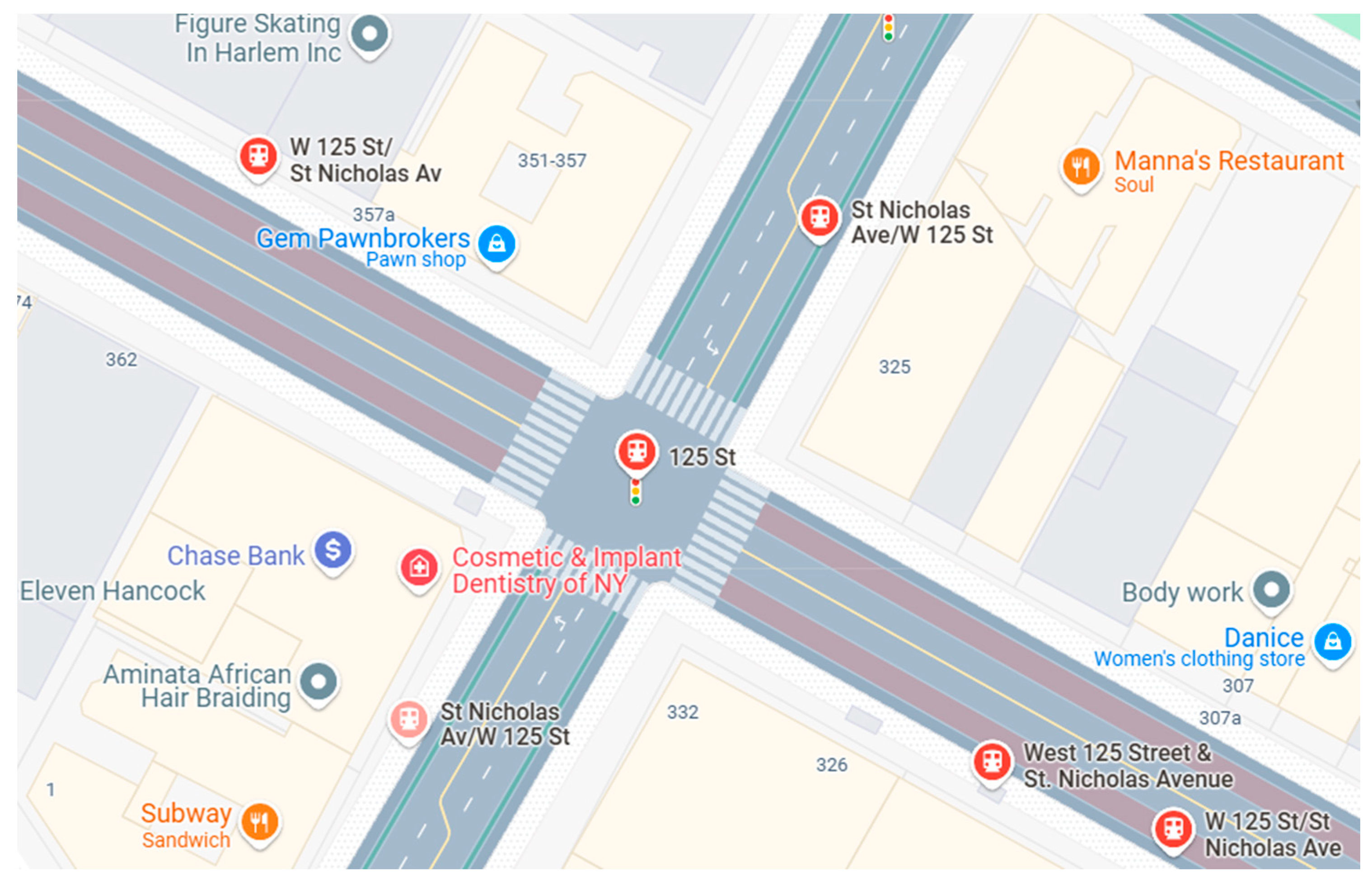
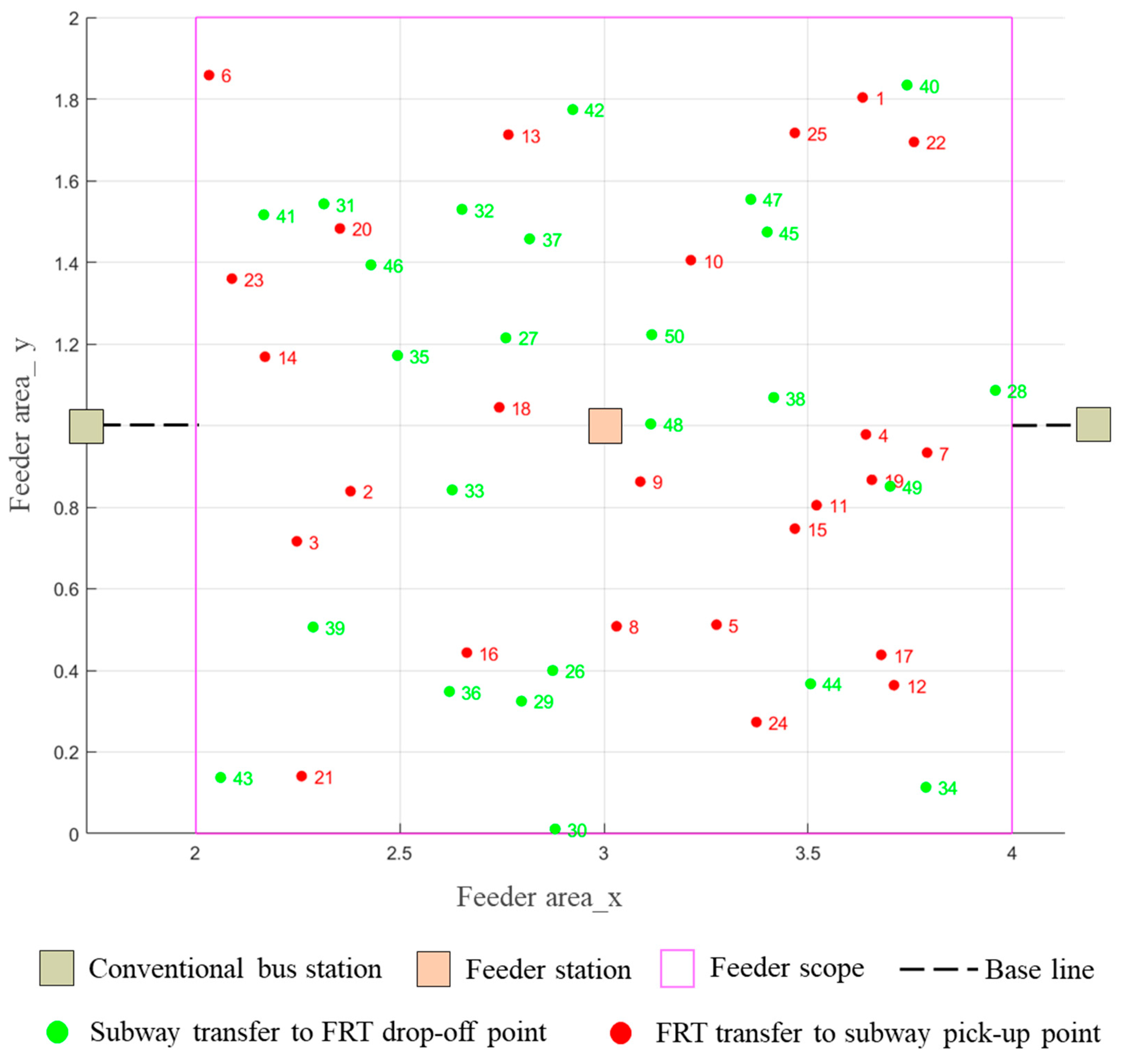
5.1. Case Description
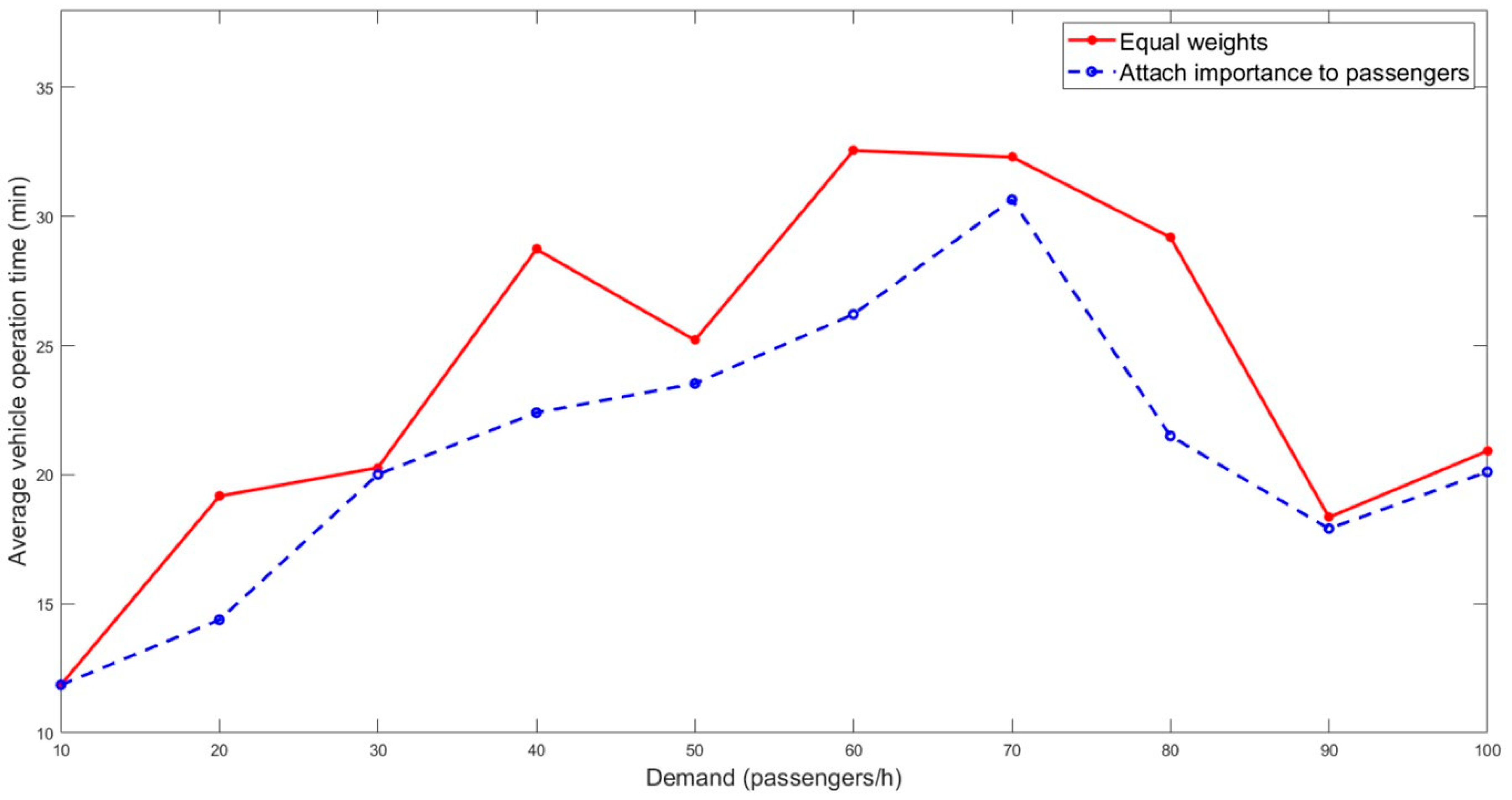
5.2. Case Analysis
6. Conclusions
Author Contributions
Funding
Institutional Review Board Statement
Informed Consent Statement
Data Availability Statement
Conflicts of Interest
References
- Liyanage, S.; Dia, H.; Duncan, G.; Abduljabbar, R. Evaluation of the Impacts of On-Demand Bus Services Using Traffic Simulation. Sustainability 2024, 16, 8477. [Google Scholar] [CrossRef]
- Fittante, S.R.; Lubin, A. Adapting the Swedish service route model to suburban transit in the United States. Transp. Res. Rec. 2015, 2563, 52. [Google Scholar] [CrossRef]
- Tolić, I.H.; Nyarko, E.K.; Ceder, A. Optimization of Public Transport Services to Minimize Passengers’ Waiting Times and Maximize Vehicles’ Occupancy Ratios. Electronics 2020, 9, 360. [Google Scholar] [CrossRef]
- Delle Site, P.; Filippi, F. Service Optimization for Bus Corridors with Short-Turn Strategies and Variable Vehicle Size. Transp. Res. Part A Policy Pract. 1998, 32, 19–38. [Google Scholar] [CrossRef]
- Sun, S.; Szeto, W.Y. Optimal Sectional Fare and Frequency Settings for Transit Networks with Elastic Demand. Transp. Res. Part B Methodol. 2019, 127, 147–177. [Google Scholar] [CrossRef]
- Tsai, F.M.; Chien, S.; Wei, C.H. Joint Optimization of Temporal Headway and Differential Fare for Transit Systems Considering Heterogeneous Demand Elasticity. J. Transp. Eng. 2013, 139, 30–39. [Google Scholar] [CrossRef]
- Zhang, J.L.; Yang, H. Transit Operations with Deterministic Optimal Fare and Frequency Control. Transp. Res. Procedia 2016, 14, 313–322. [Google Scholar] [CrossRef]
- Wang, J.; Yuan, Z. Optimization model of bus bridging scheduling with passengers transferring from urban rail transit. J. Southeast Univ. (Nat. Sci. Ed.) 2021, 51, 161–170. [Google Scholar] [CrossRef]
- Dou, X.; Meng, Q. Feeder bus timetable design and vehicle size setting in peak hour demand conditions. Transp. Res. Rec. 2019, 2673, 321–332. [Google Scholar] [CrossRef]
- Xiong, J.; He, Z.; Guan, W.; Ran, B. Optimal timetable development for community shuttle network with metro stations. Transp. Res. Part C Emerg. Technol. 2015, 60, 540–565. [Google Scholar] [CrossRef]
- Liu, J.; Wu, X. Research of emergency feeder bus scheme for urban rail transit under unexpected incident. IOP Conf. Ser. Mater. Sci. Eng. 2019, 688, 044040. [Google Scholar] [CrossRef]
- Chen, Y.; An, K. Integrated optimization of bus bridging routes and timetables for rail disruptions. Eur. J. Oper. Res. 2021, 295, 484–498. [Google Scholar] [CrossRef]
- Jin, J.G.; Teo, K.M.; Odoni, A.R. Optimizing bus bridging services in response to disruptions of urban transit rail networks. Transp. Sci. 2016, 50, 790–804. [Google Scholar] [CrossRef]
- Liang, J.; Wu, J.; Qu, Y.; Yin, H.; Qu, X.; Gao, Z. Robust bus bridging service design under rail transit system disruptions. Transp. Res. Part E Logist. Transp. Rev. 2019, 132, 97–116. [Google Scholar] [CrossRef]
- Michaelis, M.; Schöbel, A. Integrating line planning, timetabling, and vehicle scheduling: A customer-oriented heuristic. Public Transp. 2009, 1, 211–232. [Google Scholar] [CrossRef]
- Kaspi, M.; Raviv, T. Service-oriented line planning and timetabling for passenger trains. Transp. Sci. 2013, 47, 295–311. [Google Scholar] [CrossRef]
- van der Hurk, E.; Koutsopoulos, H.N.; Wilson, N.; Kroon, L.G.; Maróti, G. Shuttle planning for link closures in urban public transport networks. Transp. Sci. 2016, 50, 947–965. [Google Scholar] [CrossRef]
- Cao, Z.; Ceder, A. Autonomous shuttle bus service timetabling and vehicle scheduling using skip-stop tactic. Transp. Res. Part C Emerg. Technol. 2019, 102, 370–395. [Google Scholar] [CrossRef]
- Shang, H.; Huang, H.; Wu, W. Bus timetabling considering passenger satisfaction: An empirical study in Beijing. Comput. Ind. Eng. 2019, 135, 1155–1166. [Google Scholar] [CrossRef]
- Wu, J.; Liu, M.; Sun, H.; Li, T.; Gao, Z.; Wang, D.Z. Equity-based timetable synchronization optimization in urban subway network. Transp. Res. Part C Emerg. Technol. 2015, 51, 1–18. [Google Scholar] [CrossRef]
- Wu, Y.; Yang, H.; Tang, J.; Yu, Y. Multi-objective re-synchronizing of bus timetable: Model, complexity and solution. Transp. Res. Part C Emerg. Technol. 2016, 67, 149–168. [Google Scholar] [CrossRef]
- Associates, I. TRB’s Transit Cooperative Research Program (TCRP) Report 100: Transit Capacity and Quality of Service Manual, 2nd ed.; Transportation Research Board: Washington, DC, USA, 2003. [Google Scholar]
- Yang, X.; Teng, J. Handbook of Public Transport Capacity and Service Quality; China Construction Industry Press: Shanghai, China, 2010. [Google Scholar]
- Ceder, A.; Guan, W. Public Transport Planning and Operation: Theory, Modeling and Application; Tsinghua University Press: Beijing, China, 2010. [Google Scholar]
- Qiu, F.; Li, W.; Shen, J. Two-stage model for flex-route transit scheduling. J. Southeast Univ. (Nat. Sci. Ed.) 2014, 44, 1078–1084. [Google Scholar] [CrossRef]
- Zheng, Y.; Li, W.; Qiu, F. A slack arrival strategy to promote flex-route transit services. Transp. Res. Part C Emerg. Technol. 2018, 92, 442–455. [Google Scholar] [CrossRef]
- Quadrifoglio, L.; Dessouky, M.M.; Palmer, K. An insertion heuristic for scheduling Mobility Allowance Shuttle Transit (MAST) services. J. Sched. 2007, 10, 25–40. [Google Scholar] [CrossRef]
- Zheng, Y.; Li, W.; Qiu, F.; Wei, H. The benefits of introducing meeting points into flex-route transit services. Transp. Res. Part C Emerg. Technol. 2019, 106, 98–112. [Google Scholar] [CrossRef]
- Quadrifoglio, L.; Hall, R.W.; Dessouky, M.M. Performance and design of Mobility Allowance Shuttle Transit services: Bounds on the maximum longitudinal velocity. Transp. Sci. 2006, 40, 351–363. [Google Scholar] [CrossRef]
- Qiu, F.; Li, W.; Zhang, J. A Dynamic Station Strategy to Improve the Performance of Flex-Route Transit Services. Transp. Res. Part C Emerg. Technol. 2014, 48, 229–240. [Google Scholar] [CrossRef]


| H (min) | Demand Levels (Passengers/h) | |||||||||
|---|---|---|---|---|---|---|---|---|---|---|
| 10 | 20 | 30 | 40 | 50 | 60 | 70 | 80 | 90 | 100 | |
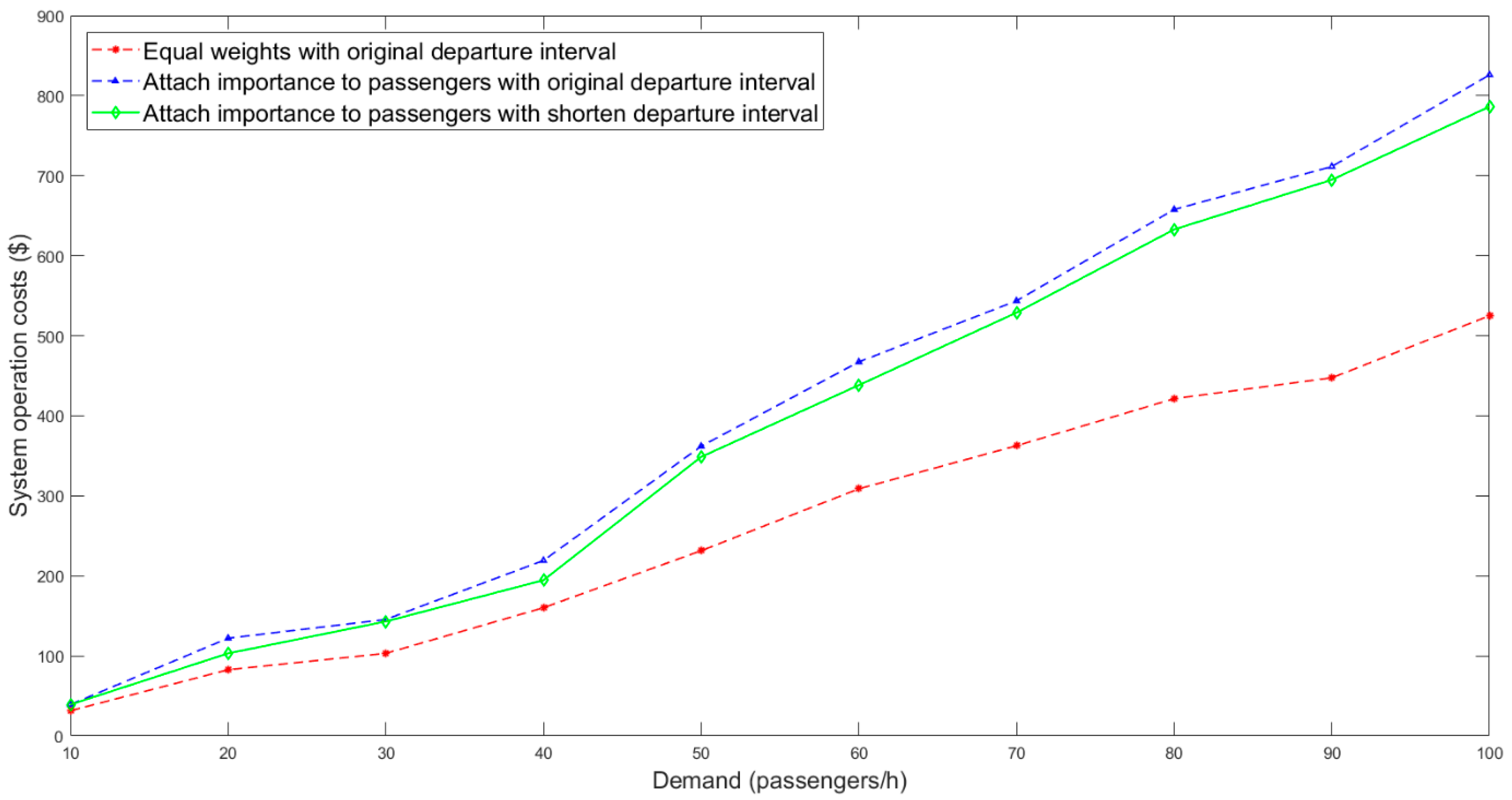
| Equal weights | 30 | 30 | 20 | 20 | 15 | 15 | 12 | 10 | 6 | 6 |
| Attach importance to passengers | 30 | 20 | 20 | 15 | 12 | 10 | 10 | 6 | 5 | 5 |
| Demand Levels (Passengers/h) | H (min) | U (USD) | Average Vehicle Running Time (min) | Number of Departure Shifts | Rejection Rate (%) |
|---|---|---|---|---|---|
| 10 | 30 | 31.46 | 11.86 | 2 | 0 |
| 20 | 30 | 82.71 | 19.17 | 2 | 5 |
| 30 | 20 | 103.16 | 20.27 | 3 | 0 |
| 40 | 20 | 160.18 | 28.73 | 3 | 7.5 |
| 50 | 15 | 231.41 | 25.21 | 4 | 0 |
| 60 | 15 | 308.76 | 32.55 | 4 | 6.67 |
| 70 | 12 | 362.57 | 32.30 | 5 | 5.71 |
| 80 | 10 | 421.44 | 29.19 | 6 | 2.5 |
| 90 | 6 | 447.48 | 18.35 | 10 | 0 |
| 100 | 6 | 525.12 | 20.92 | 10 | 3 |
| Vehicle Shifts | Departure Time of Interchange Station | Vehicle Running Path | Cumulative Number of Passengers |
|---|---|---|---|
| 1 | 7:13 | 14-2-13-10-9-0-50-32-35-26-38-49 | 11 |
| 2 | 7:23 | 6-3-12-25-0-41-29-44-40 | 8 |
| 3 | 7:33 | 23-16-5-11-1-0-42-33-36-28 | 9 |
| 4 | 7:43 | 18-4-7-19-15-17-0-27-46-43-30-48-47 | 12 |
| 5 | 7:53 | 20-21-24-8-0-37-31-39-34-45 | 9 |
Disclaimer/Publisher’s Note: The statements, opinions and data contained in all publications are solely those of the individual author(s) and contributor(s) and not of MDPI and/or the editor(s). MDPI and/or the editor(s) disclaim responsibility for any injury to people or property resulting from any ideas, methods, instructions or products referred to in the content. |
© 2025 by the authors. Licensee MDPI, Basel, Switzerland. This article is an open access article distributed under the terms and conditions of the Creative Commons Attribution (CC BY) license (https://creativecommons.org/licenses/by/4.0/).
Share and Cite
Wang, Y.; Li, Q.; Han, Z.; Zhang, J. Coordinated Optimization of Feeder Flex-Route Transit Scheduling for Urban Rail Systems. Appl. Sci. 2025, 15, 4342. https://doi.org/10.3390/app15084342
Wang Y, Li Q, Han Z, Zhang J. Coordinated Optimization of Feeder Flex-Route Transit Scheduling for Urban Rail Systems. Applied Sciences. 2025; 15(8):4342. https://doi.org/10.3390/app15084342
Chicago/Turabian StyleWang, Yabin, Qiangqiang Li, Zhenfeng Han, and Jin Zhang. 2025. "Coordinated Optimization of Feeder Flex-Route Transit Scheduling for Urban Rail Systems" Applied Sciences 15, no. 8: 4342. https://doi.org/10.3390/app15084342
APA StyleWang, Y., Li, Q., Han, Z., & Zhang, J. (2025). Coordinated Optimization of Feeder Flex-Route Transit Scheduling for Urban Rail Systems. Applied Sciences, 15(8), 4342. https://doi.org/10.3390/app15084342