Abstract
In engineering practice, many foundations are forced to be placed on slopes, whose stability is deeply affected by seismic force. Therefore, an accurate assessment of the seismic bearing capacity of strip foundations close to slopes is a crucial guide for engineering. Herein, an analytical procedure considering pseudo-dynamic influence is proposed, which offers a new assessment framework for seismic bearing capacity of strip foundations close to slopes on non-uniform soils. Considering the temporal and spatial characteristics of earthquake action, the seismic bearing capacity of foundations at different normalized frequencies is obtained, and depth profiles of seismic acceleration coefficients at different normalized frequencies are presented. The consistency between this paper’s computational results and the published literature substantiates the dependability of the proposed analytical procedure. The sensitivity analyses are carried out for horizontal seismic coefficients, normalized frequencies, damping ratios, internal friction angles, slope angles, cohesion, and non-uniform coefficients, and the results are presented for practice reference in engineering.
1. Introduction
In many cases where foundations have to be placed near slopes, slope instability under the seismic effect is one of the most common geological disasters in engineering, which is a great threat to people’s lives and property safety. Therefore, the accurate assessment of seismic bearing capacity of strip foundation has an indispensable role in guiding actual engineering, which has attracted the attention of many scholars.
The calculation methods of foundation bearing capacity are mainly classified into the following four types: (a) slip line method, (b) limit equilibrium method, (c) limit analysis method, and (d) numerical simulation. Because of the simplicity of the limit analysis method, it has been employed by many scholars. Compared with the later emerging numerical simulation, including the finite element method and the discrete element method, the limit analysis method can quickly obtain many calculation results to carry out parameter analysis to explore the influence of different parameters. However, it is difficult to use the limit analysis method to deal with some complex working conditions. In addition, the limit analysis approach comprises two distinct methodologies: the upper bound and lower bound techniques. The upper bound methodology employs the virtual work principle to determine the maximum possible bearing capacity through analysis of kinematically admissible velocity fields, while the lower bound method obtains the lower bound value of bearing capacity from the static permissible stress field by using the stress equilibrium. Soubra (1999) [1] provided a method for the assessment of the bearing capacity of the foundations based on the upper bound method of the limit analysis based on the two different failure mechanisms and verified the validity of the method.
This field has attracted the attention of many scholars due to the growth of cases where foundations are placed on adjacent slopes. Based on the method of Soubra (1999) [1], Saada et al. (2011) [2] similarly calculated the seismic bearing capacity of strips near rock slopes for different failure mechanisms using the upper bound method. Raj (2018) [3] evaluated the seismic bearing capacity of foundations near and soil slope using finite element limit analysis upper limit method (FELA) and finite element limit analysis lower limit method, respectively. Wu et al. (2021) [4] calculated the ultimate bearing capacity of strip foundations on rock slopes by using FELA. Wu et al. (2023) [5] gave the seismic bearing capacity of strip foundations on rock slopes under eccentric loading conditions by using the FELA method. Keshavarz et al. (2024) [6] investigated the bearing capacity of foundations on rock slopes based on slip line method and FELA method.
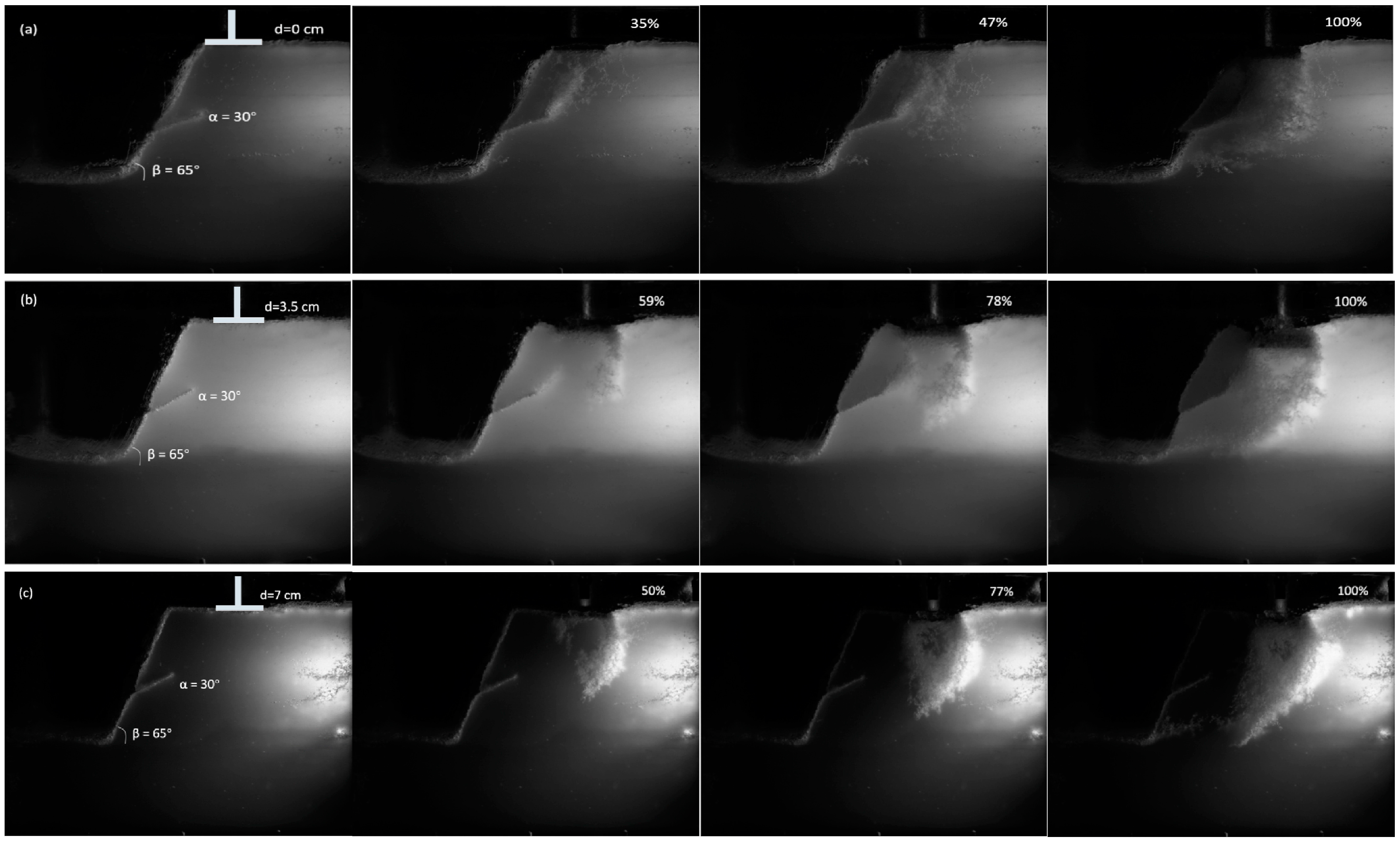
It is to be noted that there are currently three main methods of dealing with seismic forces. The first method is known as the pseudo-static method (PS), which is widely used because of its simplicity. This method uses a constant coefficient to characterize the magnitude of lateral or vertical seismic forces, and, therefore, most scholars believe that the pseudo-static method can only simply represent the dynamic properties of seismic forces (through the variation of ), ignoring the time factor. The second method is the conventional pseudo-dynamic method (CPD). Considering the phase difference in seismic waves in the backfill and the amplification effect, Steedman and Zeng (1990) [7] gave a means of the pseudo-dynamic analysis of the active earth thrust of a retaining wall. Subsequently, the method was adopted and further extended by many scholars [8,9,10]. The method assumes that both pressure and shear seismic waves are upward-propagating harmonics, which have the same frequency but different amplitudes. Although the conventional pseudo-dynamic method has been widely used in the field of seismic stability analysis of geotechnical engineering, it still has some disadvantages. By derivation, it can be found that the seismic wave equation assumed in the method does not satisfy the boundary condition that the stress at the soil surface should be zero. This is since the method assumes that the seismic wave is an upward propagating harmonic wave, whereas the wave in the actual soil is generated by constructive interference between the upward propagating wave and the wave reflected through the free surface of the soil. Therefore, based on the visco-elastic model and considering the effect of soil damping ratio as well as the above-mentioned boundary conditions, Bellezza (2014) [11] came up with an advanced and modified pseudo-dynamic method (MPD). As shown in Figure 1, Wei et al. (2023) [12] conducted model tests using the transparent soil technique, present the initiation and propagation of slip surfaces. Kang et al. (2024a) [13] evaluated the modified pseudo-dynamic bearing capacity of reinforced soil foundation based on three reinforcement mechanisms. Tan and Vanapalli (2022) [14] evaluate the bearing capacity of a strip foundation located on an unsaturated soil slope under the influence of different rainfall infiltration conditions. By adopting the Mohr–Coulomb (MC) yield criterion, Kumar and Korada (2022) [15] employed the method of stress characteristics (MOSC) to evaluate the bearing capacity factor Nγ for rough strip footings subjected to horizontal pseudo-static earthquake inertial forces on sloping ground surfaces. Peng et al. (2021) [16] established an asymmetric failure mechanism for laterally loaded piles on slopes, deriving analytical bearing capacity solutions through limit analysis and proposing a dimensionless capacity ratio. This ratio exhibits a near-linear relationship with normalized pile-slope distance until reaching a critical threshold where slope effects vanish.

Figure 1.
Process of shear band propagation with different setback distances of the footing. (a) d = 0 cm; (b) d = 3.5 cm; (c) d = 7 cm [12].
Although there have been many studies on the seismic bearing capacity of foundations near slopes. However, most of the existing studies are based on the pseudo-static method or the conventional pseudo-dynamic method. The spatial–temporal patterns of seismic forces cannot be effectively characterized through this methodology. Therefore, herein, a new framework for seismic capacity assessment of foundations near slopes considering the non-uniformity of the soil is proposed based on the limit analysis and modified pseudo-dynamic method. It is assumed that the cohesion of the soil grows linearly along the depth to represent the non-uniform characteristics. Finally, comparisons and parametric analyses are carried out. The agreement shows that the proposed method is correct.
2. Theoretical Framework for Seismic Bearing Capacity
2.1. Upper Bound Theorem of Limit Analysis
Limit analysis is used to assess different types of geotechnical stability problems due to its solid theoretical foundation and ease of use [17]. Limit analysis consists of an upper bound method and a lower bound method, in which the first method refers to the bearing capacity that is greater than the actual damage load based on the assumed reasonable failure mechanism and energy consumption balance, while the second method refers to the bearing capacity that is not greater than the actual damage load based on the stress balance and yield condition. In this paper, the upper bound theorem is adopted, which can be expressed as Equation (1). The specific calculation process is as follows: firstly, a velocity field conforming to kinematics is assumed, and then based on this velocity field, the upper bound solution of the bearing capacity can be found when the external power is equal to the internal energy dissipation. In addition, it is to be noted that seismic forces are considered as external forces.
In order to use the Upper bound theorem of limit analysis, the following assumptions need to be met:
- Soil material is an ideal elastic-plastic material;
- The soil satisfies the assumption of small deformation;
- Drucker postulate.
2.2. Modified Pseudo-Dynamic Method
Using limit analysis of bearing capacity, the most critical issue is how to quantify the seismic force, which is considered as an external force by all existing methods. Assume seismic S- and P-wave are harmonic waves propagating upward with different amplitudes and the same frequencies. According to the above, at present, there are roughly three treatments including PS, CPD, and MPD. PS represents the seismic force acceleration coefficients by a constant, and the seismic acceleration coefficients of CPD are shown in Equations (2) and (3).
where and are the initial seismic acceleration coefficients for horizontal and vertical at , respectively, and H is the height of the retaining wall; is the amplification factor, is the frequency, t is the time, and and are the wave velocities of shear and pressure waves, respectively. Bellezza (2014) [11] gave the modified pseudo-dynamic method with the following formulation:
where means the velocity of the shear wave, and both are constants, means the damping ration of soils, means the depth from bedrock, means the coefficient of the seismic acceleration, and means the seismic acceleration.
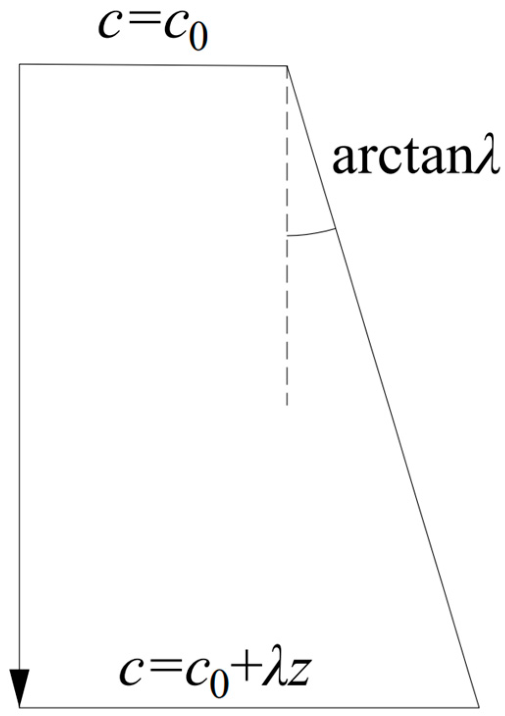
2.3. Non-Uniform Soil Profile
Due to different stress histories, depositional methods, and consolidation pressures, soils often exhibit non-homogeneous properties, and, in general, their non-homogeneity is mainly reflected in the depth direction. Different scholars have made different quantitative assumption models for the non-homogeneous characteristics of soils [18,19,20,21]. In this paper, the model based on the classical linear Mohr–Coulomb criterion is adopted, in which the cohesion of soils and the distance from the surface of soils tend to increase linearly, as shown in Figure 2. As the assumption is ideal and simple, it is more difficult to accurately reflect the real non-uniform properties of soils. However, the comparative analysis between the numerical results obtained in this paper and previously published data confirms the dependability of the computational methodology employed.
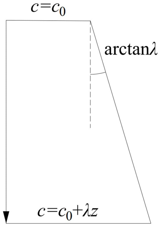
Figure 2.
The depth profile of cohesion.
3. Upper Bound Analysis of Seismic Bearing Capacity
Based on the above theoretical framework, this section details the derivation and computational procedure of the upper bound analysis of the modified pseudo-dynamic bearing capacity for the foundation near slope.
3.1. Failure Mechanism
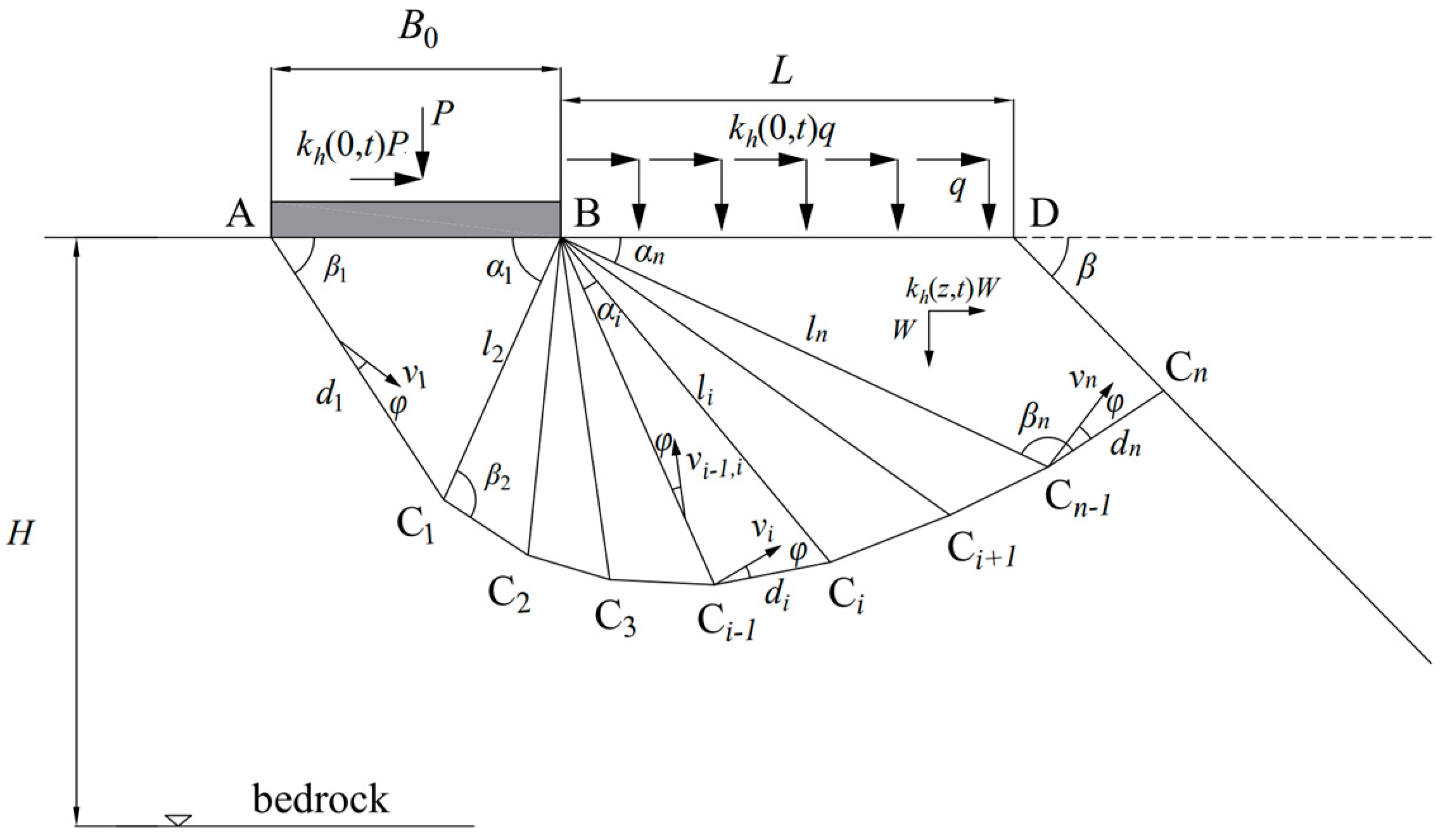
Based on the definition and formulation of the upper bound theorem, it can be found that the most critical step is to determine an accurate velocity-permissive motion field (failure mechanism), and the failure mechanism can reflect the real damage of the foundation more accurately. Therefore, based on the conclusions of previous studies (Soubra, 1999 [1]; Kang et al., 2024 [22]), the failure mechanism shown in Figure 3 is established in this paper. Since the effect of seismic action is considered in this paper, the damage pattern of the foundation is unilateral.
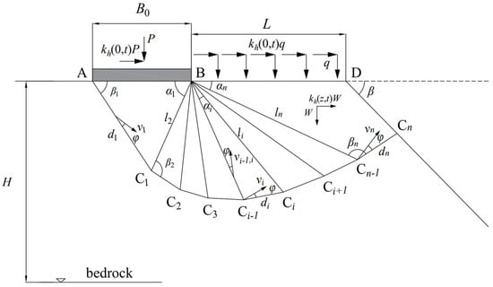
Figure 3.
The geometry and force diagram of unilateral failure mechanism.
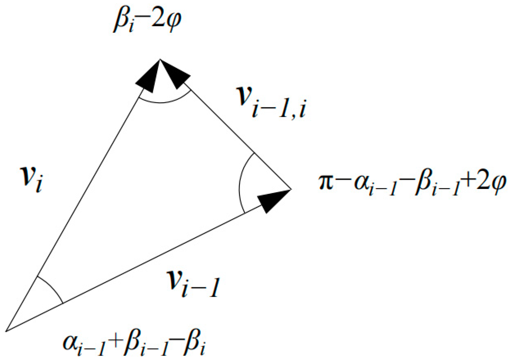
The failure mechanism is a multi-block wedge structure with a total of n blocks, including n − 1 triangular blocks and one quadrilateral block [23,24,25]. From Figure 3, it can be found that the block ABC1 at the bottom of the foundation moves in the direction of velocity at a certain angle to the rupture surface AC1, and the other blocks move in a similar manner as ABC1, all at a certain angle to the respective bottom rupture surface (Shan et al. (2025) [26]). In addition, the strip footing is at a certain distance L from the apex D of the slope surface, which is called the setback distance.
The external forces acting on the above mechanism are foundation load, uniform load, soil self-weight, and seismic force, while the internal energy dissipation exists on the velocity discontinuity line as well as on the rupture surface . It should be noted that, based on previous experience in the literature (Soubra (1999) [1]), the effect of vertical seismic forces on foundation bearing capacity is small. This study exclusively focuses on the impact of horizontal seismic components. In addition to this, it can be found that there are two angles in each block that are variable, including and . Therefore, by geometrical derivation, the side length of each block can be obtained as follows:
where means the area of each block. Unlike the case of surface level, when the foundation is close to the vicinity of the slope, as shown in Figure 3, the nth block is no longer a traditional triangle, but a quadrilateral, and therefore its geometric relationship needs to be derived separately and can be expressed as follows:
Furthermore, Figure 4 illustrates the relationship between the velocity vectors of the different blocks, including the overall movement velocity of the blocks as well as the velocity on the interrupted line, which can be expressed as follows:
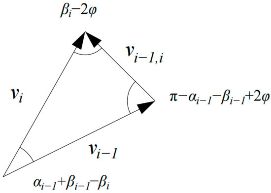
Figure 4.
The velocity diagram.
3.2. Upper Bound Calculation
In this paper, it is assumed that the soils follow the linear Mohr–Coulomb criterion. According to the previous section, for the whole foundation failure mechanism, the foundation forces, uniform forces, seismic forces, and inertial forces of the soil are the external forces, while the cohesion at the rupture surfaces as well as on the velocity discontinuity lines is the internal force. To make the power of external force doing work equal to the power of internal energy dissipation, the following equation can be obtained.
where means the work done by the external forces, means the work done by the internal forces.
Power of external forces. The calculation of the work done by the load on the upper part of the foundation is as follows:
where is shown in Figure 3, is defined in Appendix A, and means the foundation width. The power of uniform load from self-weight of overlying soils is shown as follows:
where means the setback distance, which is illustrated in Figure 3, is defined in Appendix A. The power of soil inertial force is written as follows:
where means the soil unit weight, is defined in Appendix A.
According to Equation (4), it can be found that the acceleration coefficient of the seismic force varies in depth. Based on previous experience, the horizontal seismic force is characterized by the horizontal inertia force of the soil mass. Therefore, the distribution of the horizontal force inside each individual block is not uniform, and the power of the seismic force in each block should be calculated by using an integral method [27,28]. However, due to the large number of blocks, the calculation using integration is time-consuming. Therefore, to improve the efficiency of the calculation, this paper adopts the simplified method of hierarchical calculation, and the accuracy of this method can be guaranteed. The formula is as follows:
where means the number of layers per block, means the area of the jth layer portion of the ith block, which can be expressed as , means the width of the jth layer portion of the ith block, means the height of the jth layer portion of the ith block, which can be expressed as , and . In this paper, is taken as 50.
Dissipation of internal energy. Internal energy dissipation occurs at the rupture surface as well as at the velocity discontinuity surface , but it is important to note that soil cohesion is no longer constant but increases linearly with depth. Therefore, the dissipation of internal energy on the velocity discontinuity surface can be represented by a segmentation method similar to the seismic force calculation, which can be expressed as follows:
The first term in Equation (26) is the part of the initial cohesion, while the second term is the part that grows linearly. The dissipation of internal energy on the rupture surface is shown as follows:
The above is the power formula for the internal and external work, which is brought into Equation (20) by the definition of the upper bound theorem, then the display function on the foundation bearing capacity is obtained, as shown in Equation (31), which includes variables.
4. Results and Analysis
In the above section, the formulae for the foundation bearing capacity were obtained, which included some uncertain variables; therefore, in this paper, the optimization procedure is used to obtain its optimal upper bound solution through iterations, and parametric analyses and discussions are carried out in this section.
4.1. Convergence Analysis
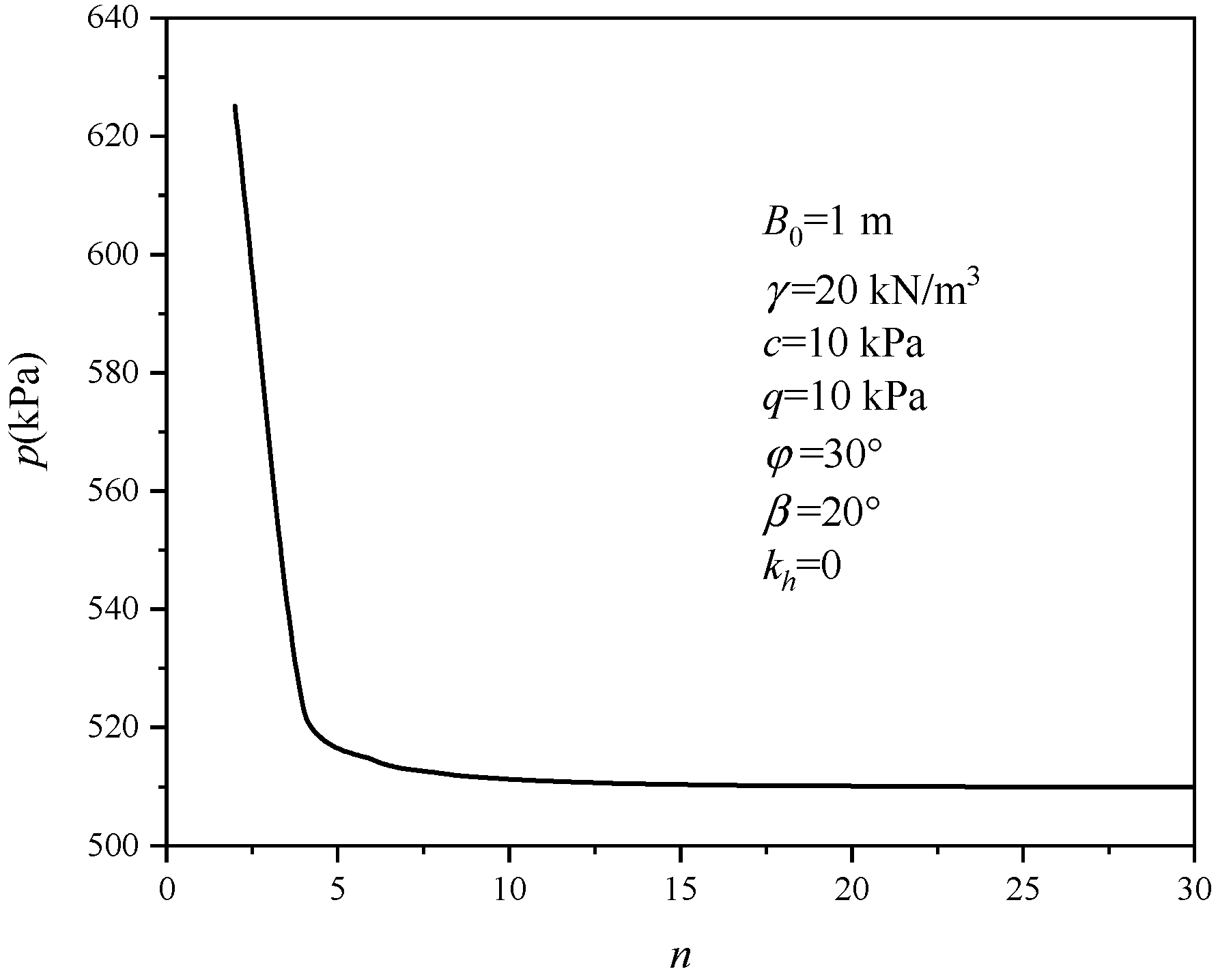
As presented above, n represents the number of wedge blocks. According to previous studies, when the number of wedge-shaped blocks is higher, the bottom rupture surface of the failure mechanism is smoother, and the calculated bearing capacity is more accurate. To take an appropriate value of n, this subsection carries out a convergence analysis of the foundation bearing capacity with respect to n, as shown in Figure 5. The specific values of the parameters are B0 = 1 m, γ = 20 kN/m3, c = 10 kPa, q = 10 kPa, φ = 30°, β = 20°, kh = 0, where seismic forces are not considered.
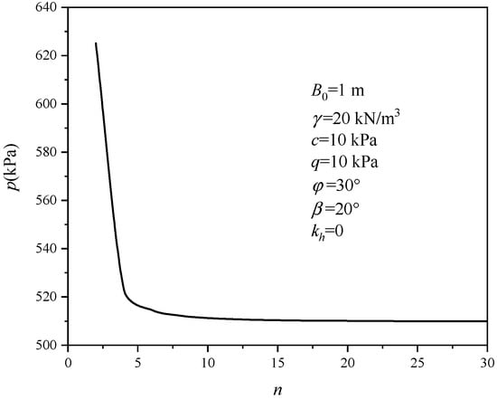
Figure 5.
The convergence of the operation program for n.
Figure 5 illustrates the trend of foundation bearing capacity with the number n of wedge blocks. The bearing capacity decreases with increasing n until it stabilizes. There is a sudden decrease in the bearing capacity between n equal to 3 and 7, and when n is more than 7, the bearing capacity performance approaches a steady state. Therefore, the bearing capacity has convergence for n. In addition, when n increases from 2 to 20, the bearing capacity decreases by about 18%, whereas when n increases from 20 to 30, the bearing capacity only decreases by about 0.04%. Therefore, to balance the accuracy and efficiency of the calculation results, in this paper, n is taken to be equal to 20.
4.2. Comparisons
4.2.1. Comparison Without Considering Seismic Forces
Before proceeding with the subsequent analyses and discussions, it is necessary to prove the reliability of the destructive mechanism proposed in the previous section. Therefore, in this subsection, the calculation results under different conditions were compared with the available data in the literature. Based on the failure mechanism presented in Figure 3, the bearing capacity of the foundations near the slope under static conditions (without considering seismic effects) was first calculated, as shown in Table 1 and Table 2. The comparison of the cohesion-dominated bearing capacity factor is given in Table 1. For the calculation of , the effect of uniform load as well as the unit weight of the soil is neglected and only the contribution of the cohesion is considered. As can be seen from Table 1, the method of this paper yields the smallest upper bound bearing capacity solution compared to the methods of the other three literature, and the results of this paper are very close to the data of Manna et al. (2021) [29]. When is equal to 0, the value of bearing capacity in this paper is about 15% smaller than the value given by Sawada et al. (1994) [30] and about 3% smaller than the value given by Askari and Farzaneh (2003) [31]. When is equal to 4, the value of bearing capacity in this paper is about 20% smaller than the value given by Sawada et al. (1994) [30] and about 12% smaller than the value given by Askari and Farzaneh (2003) [31]. The reason that the results of this paper are close to the data of Manna et al. (2021) [29] is because the same methodology was used.

Table 1.
The comparisons of with the other literature.
Table 2.
The comparisons of with the other literature.
Table 2 demonstrates the comparison of the bearing capacity factor dominated by the unit weight of soils for different internal friction angles , setback distances and slope angles considered. From Table 2, it can be seen that due to the use of upper bound theorem in both studies, the results of this paper are relatively similar to those of the other two studies. In addition, it can be noticed that at , there is a slight fluctuation in some of the bearing capacity factor from the results of the other literature, which may be due to the optimization procedure as well as the differences in the codes. The overall consistency between this study’s outcomes and the existing literature data supports the credibility of both the failure pattern interpretation and optimization approach implemented herein [32,33,34].
4.2.2. Comparison Considering Seismic Forces
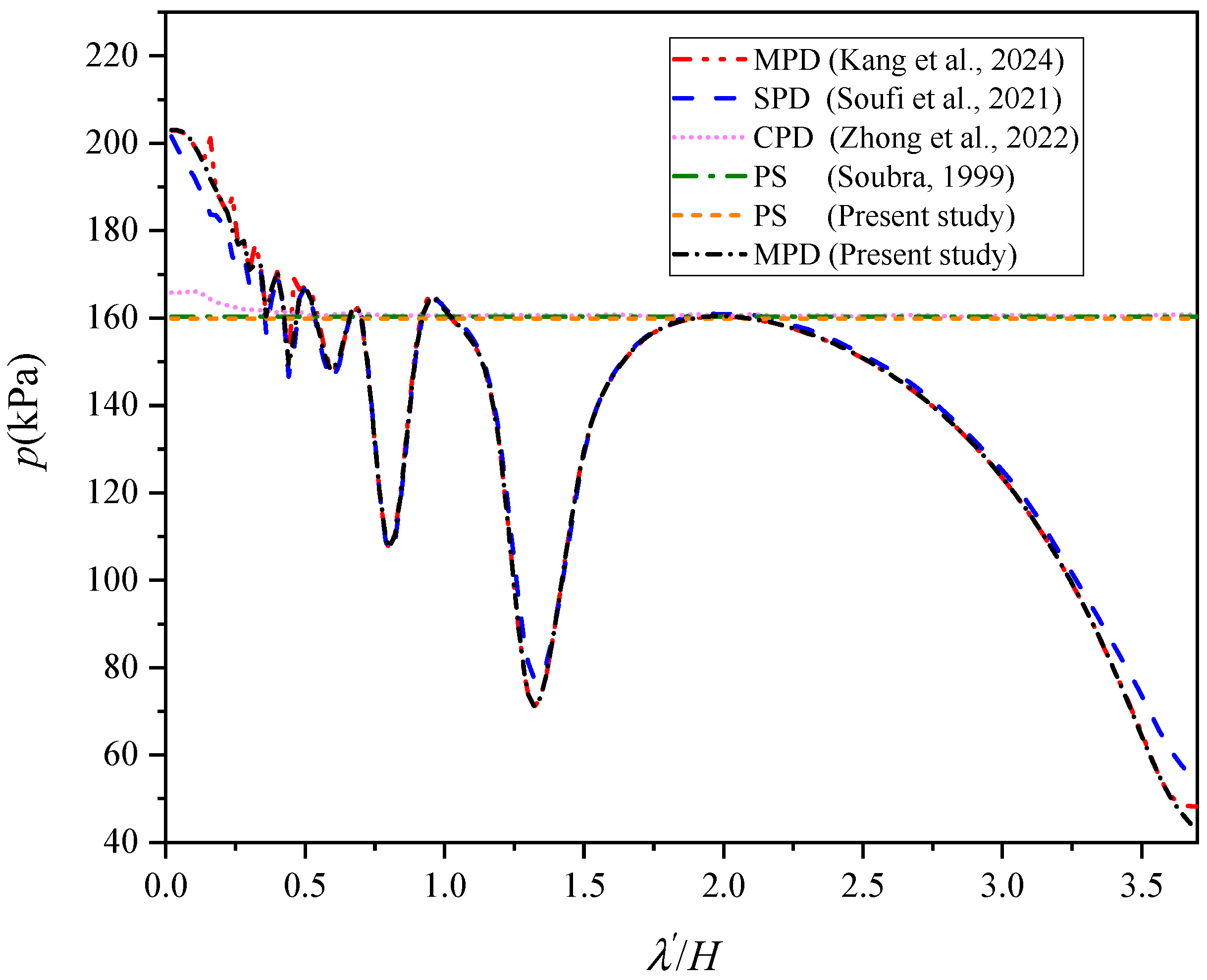
Based on the results of the previous section, it can be found that the results in the static case are very reliable, but the validity of the results when incorporating seismic forces into the limit analysis framework is still unknown; therefore, this section focuses on analyzing the seismic bearing capacity of foundations under different methods. Figure 6 shows the foundation bearing capacity calculated using different methods and the comparison with the existing literature results. It should be noted that the horizontal coordinate of Figure 6 represents the , where denotes the wavelength, which can be expressed as . Four different means of seismic force quantification are used in the results given in Figure 6, including the pseudo-static method (PS), the conventional pseudo-dynamic method (CPD), the spectral pseudo-dynamic method (SPD), and the modified pseudo-dynamic method (MPD). It should be emphasized that in order to compare the results with those of other studies, the seismic bearing capacity of strip foundations on horizontal ground is calculated in this section. It can be seen from Figure 6 that the results calculated in this paper using the MPD have the same trend and are closer to the results of Soufi et al. (2021) [33] and Kang et al. (2024) [22]. Soufi et al. (2021) [33] used the SPD to obtain the seismic bearing capacity, where the SPD is an improvement of the CPD to consider the . Kang et al. (2024) [22] also used the MPD and therefore the results are very close to those of this paper, where the slight difference may be due to the different optimization algorithms used.
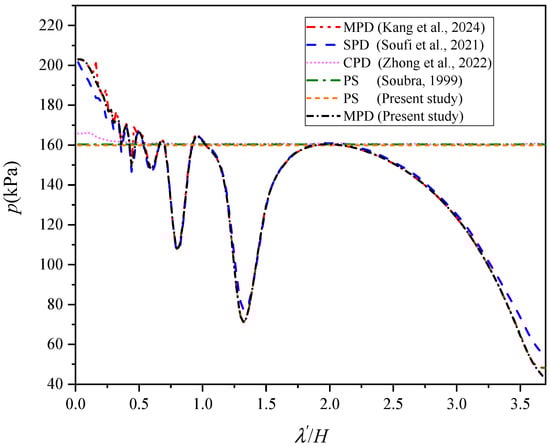
Figure 6.
The comparison of the seismic bearing capacity using the varying approaches [1,22,33,34].
The results calculated by the pseudo-static method in this paper are also very similar to those of Soubra (1999) [1] and Zhong et al. (2022) [34], which again proves the validity of the calculation process and the results in this paper. In addition, it can be found that compared with the results obtained by the PS and the MPD, the results calculated by the MPD show a completely different trend, and it can be found that there is a significant unfavorable position, so this paper is based on the MPD to accurately assess and analyze the seismic bearing capacity of the foundations near slope.
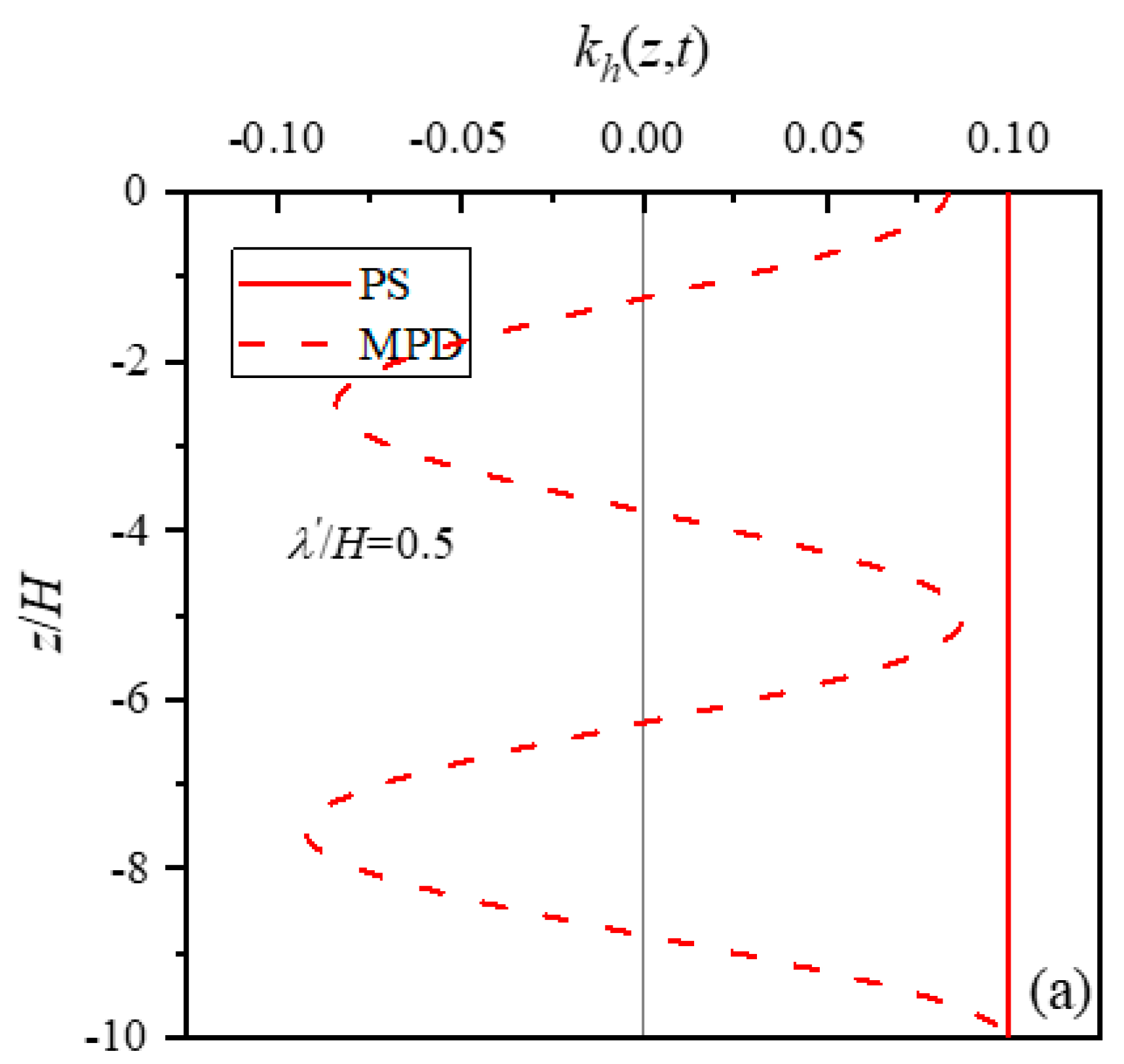
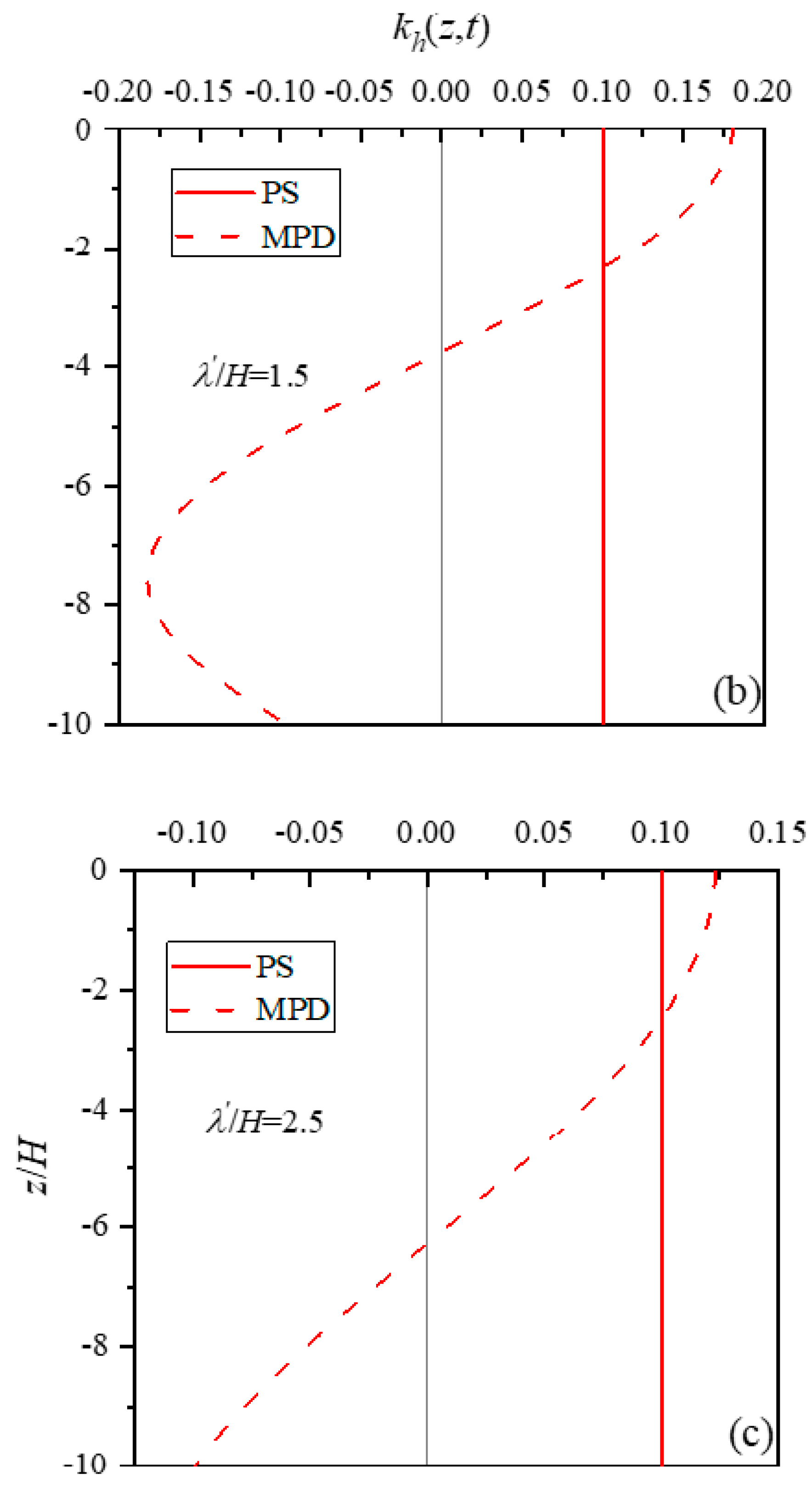
As mentioned in the analysis above, the trends of the results calculated using the pseudo-static method and the modified pseudo-dynamic method are quite different, due to the fact that these two methods use different ways to quantify the horizontal acceleration coefficients of seismic forces. The depth profiles of the horizontal acceleration coefficients of seismic forces obtained by these two methods at different are given in Figure 7. It should be noted that the same initial coefficient of seismic acceleration is assumed to be 0.1. For the pseudo-static method, regardless of the position of the soil in the soil profile, the seismic acceleration coefficient remains a constant value that will not change. While for the modified pseudo-dynamic method, its seismic acceleration coefficient always changes with depth and there is an obvious harmonic feature at , which disappears gradually as m becomes larger. When , the acceleration coefficient of the MPD fluctuates between 0.08 and −0.09, while when , the acceleration coefficient of the MPD reaches a maximum of about 0.18, and the minimum value is −0.18. It should be noted that when , the acceleration coefficient of the MPD reaches a maximum of about 0.4, which is much larger than that of the PS. In addition, it can be found that for Figure 7b–d, the acceleration coefficient of the MPD is always larger than that of the PS at the near-surface, and for the shallow strip foundations, the damage area is also often at the near-surface. This leads to significant differences in the calculation results using these two methods in some cases. In conclusion, it can be seen from Figure 7 that has a large influence on the coefficient of seismic horizontal acceleration, so it is necessary to consider the influence of when calculating the seismic bearing capacity of foundations.
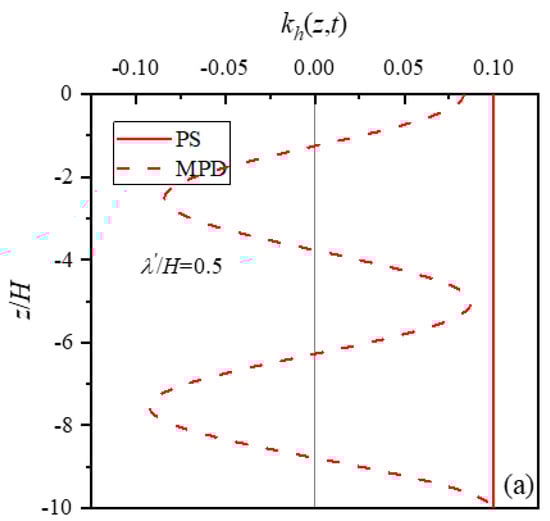
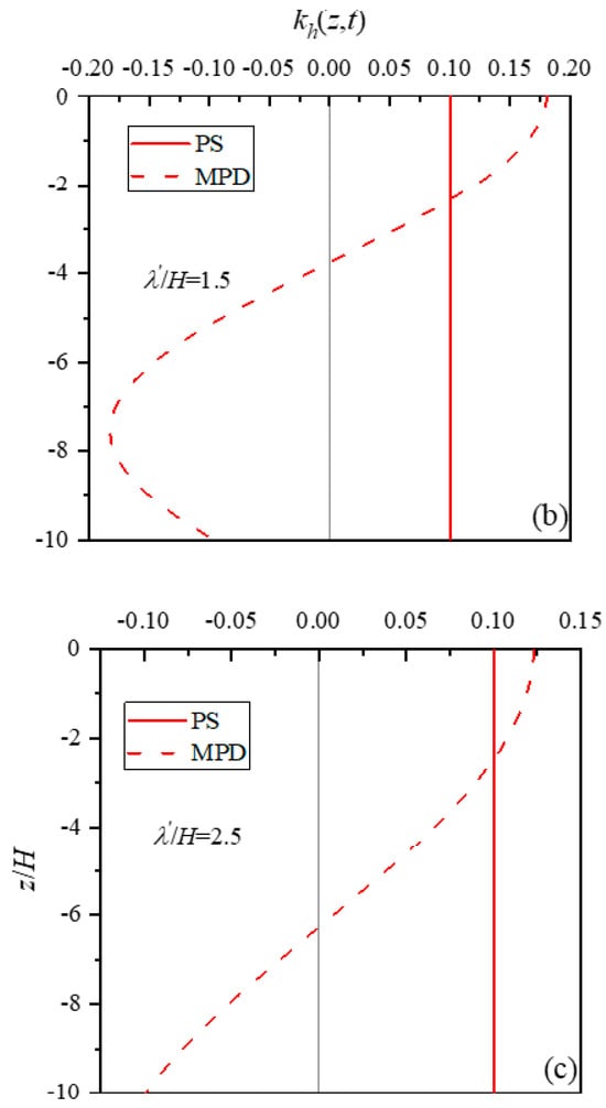
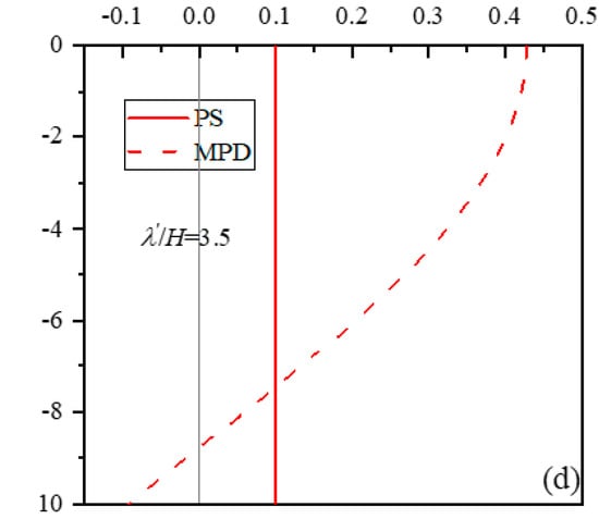
Figure 7.
The depth profiles of the seismic acceleration coefficient for the PS and the MPD. (a) λ’/H = 0.5; (b) λ’/H = 1.5; (c) λ’/H = 2.5; (d) λ’/H = 3.5.
4.3. Parameter Analysis
In this section, sensitivity analyses of different parameters are carried out and their effects on the seismic bearing capacity of foundations near slope are discussed. Unless otherwise specified, the values of the parameters are as follows: , , , , . It should be noted that the computational time required to obtain a dataset under varying parameters is approximately one minute per set.
4.3.1. Influence of and
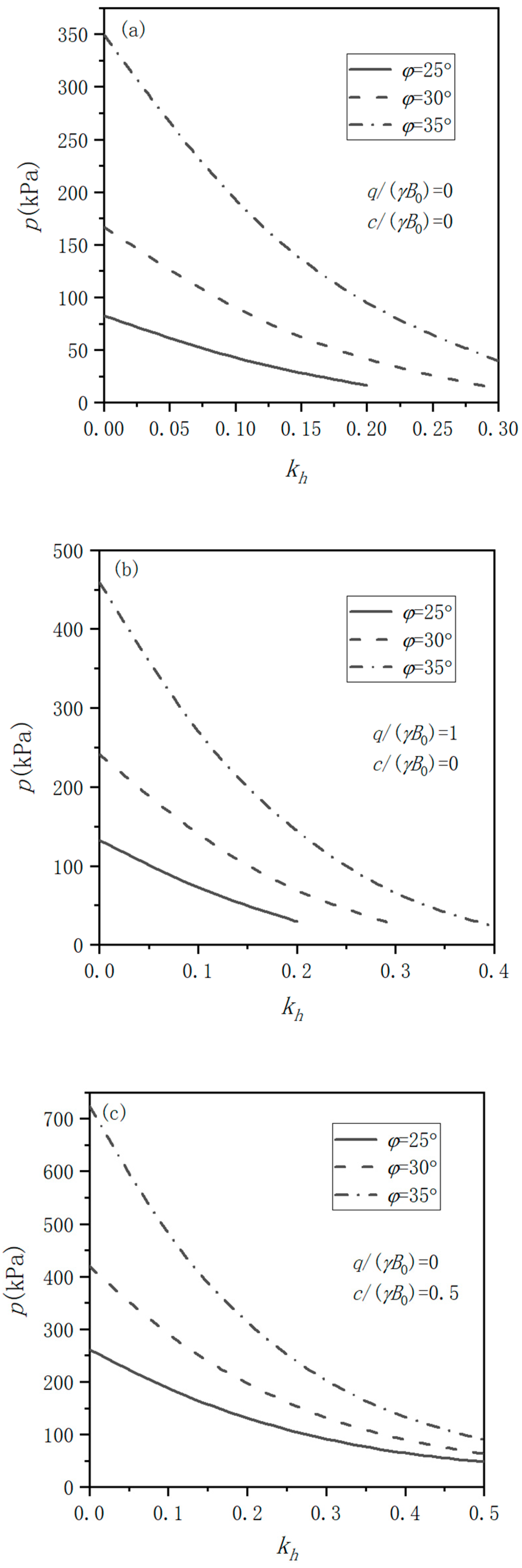
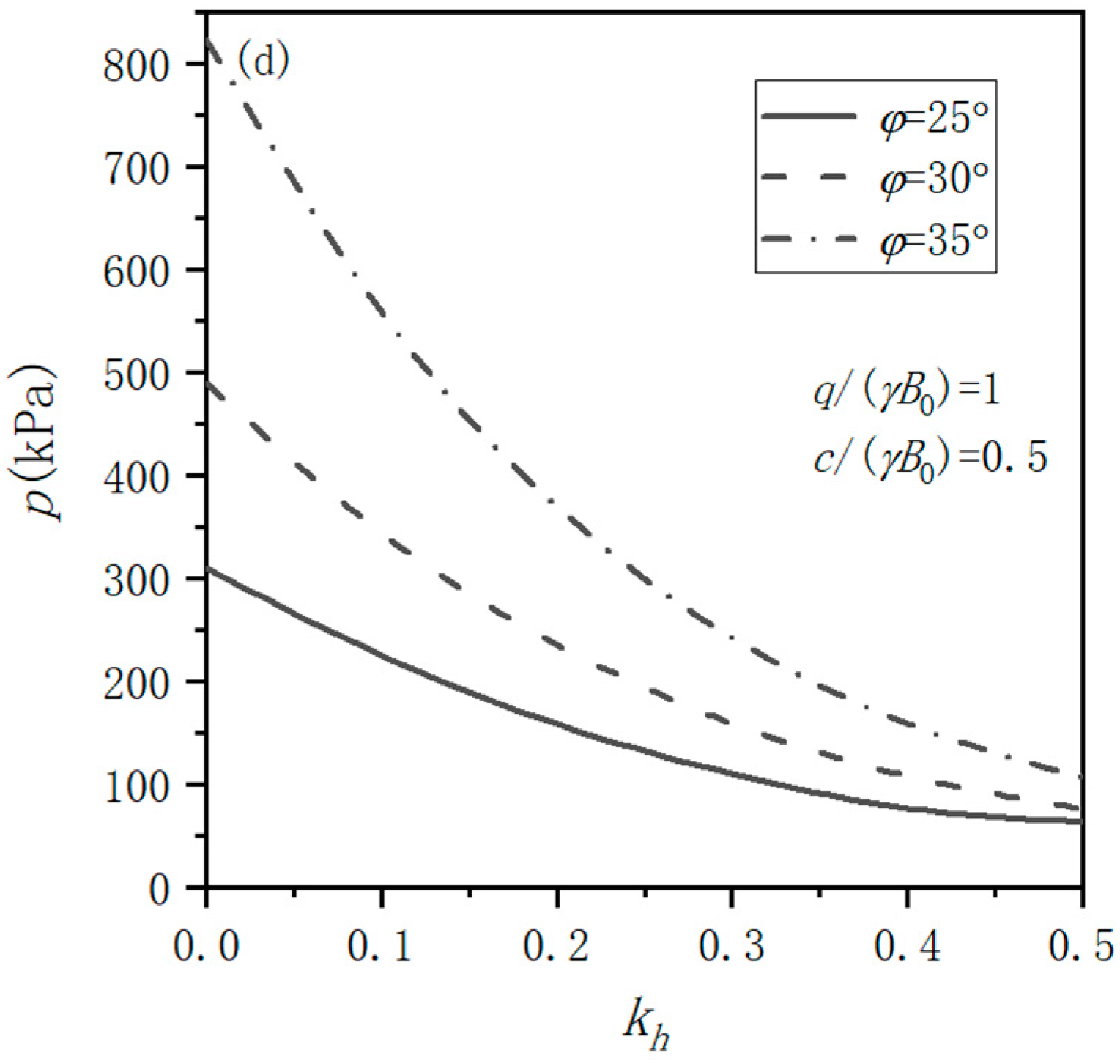
Figure 8 demonstrates the trend of seismic bearing capacity with the initial seismic acceleration coefficient for different internal friction angle . Through Figure 8, it can be found that is negatively correlated with , and decreases as increases. For Figure 8d, decreases by about 80% when increases from 0 to 0.5 for , while decreases by about 87% when increases from 0 to 0.5 for .
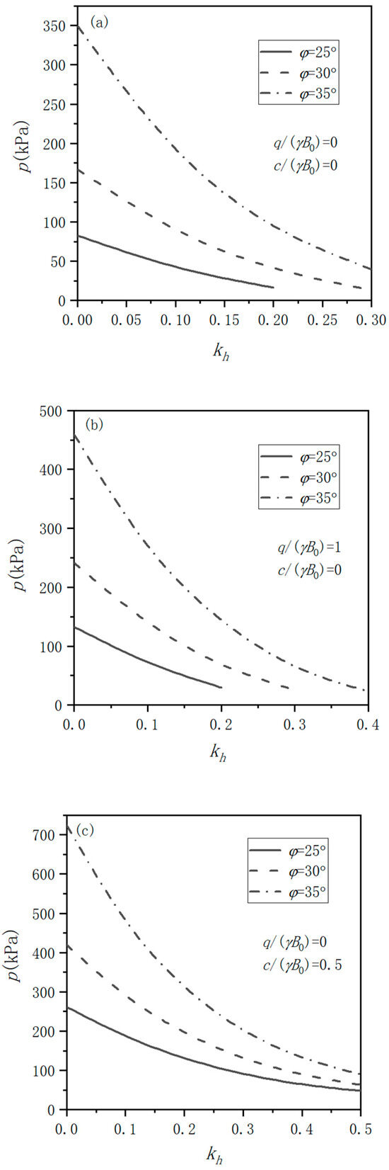
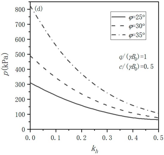
Figure 8.
The trend of the seismic bearing capacity with the initial seismic acceleration coefficient at different . (a) , ; (b) , ; (c) , ; (d) , .
In addition, is positively correlated with , with increasing as increases. For Figure 8a, increases by about 320% as increases from 25° to 35° when , while increases by about 480% as increases from 25° to 35° when . Furthermore, it can be seen that the gap between the curves for different decreases as increases.
4.3.2. Influence of and
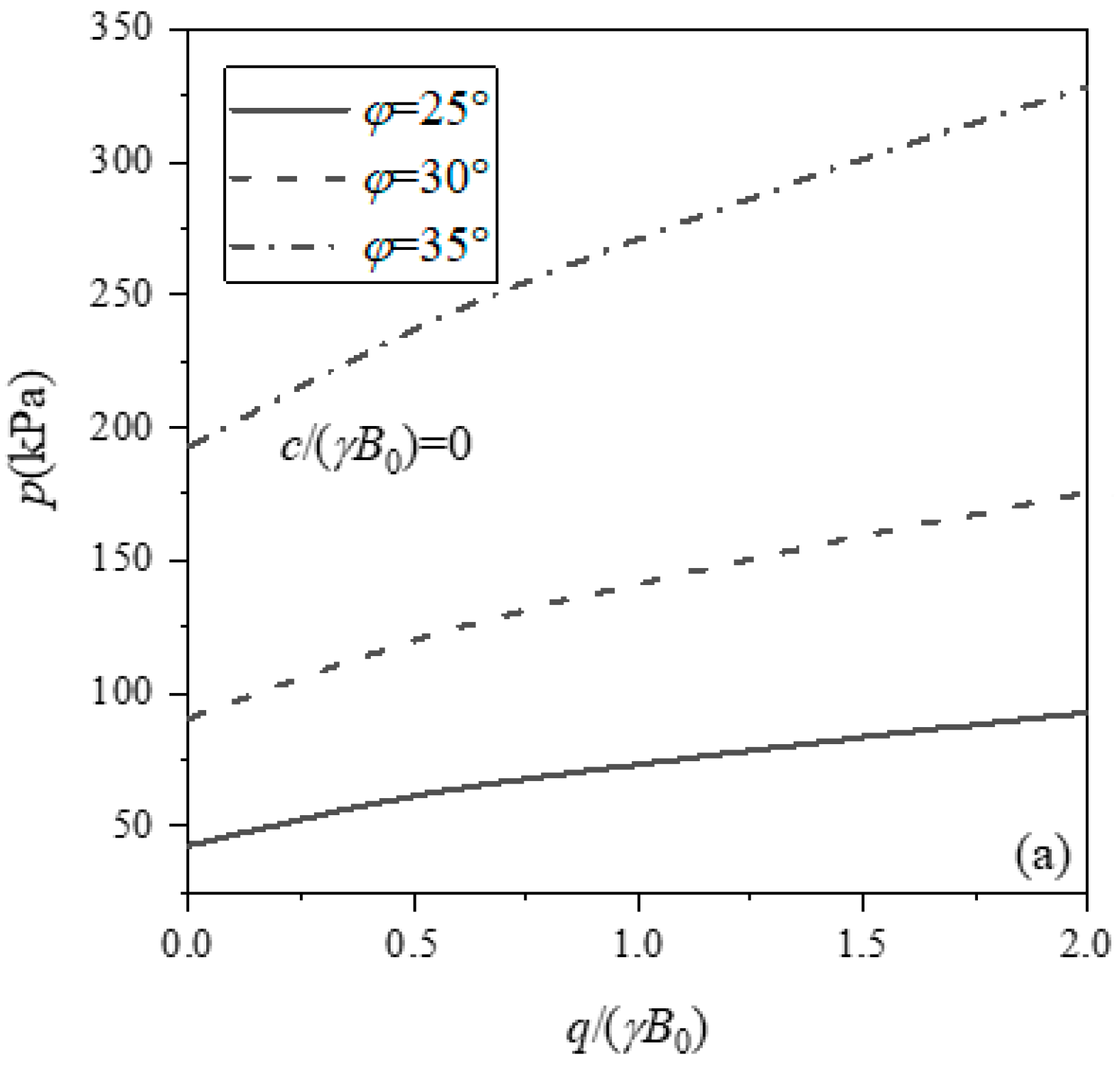
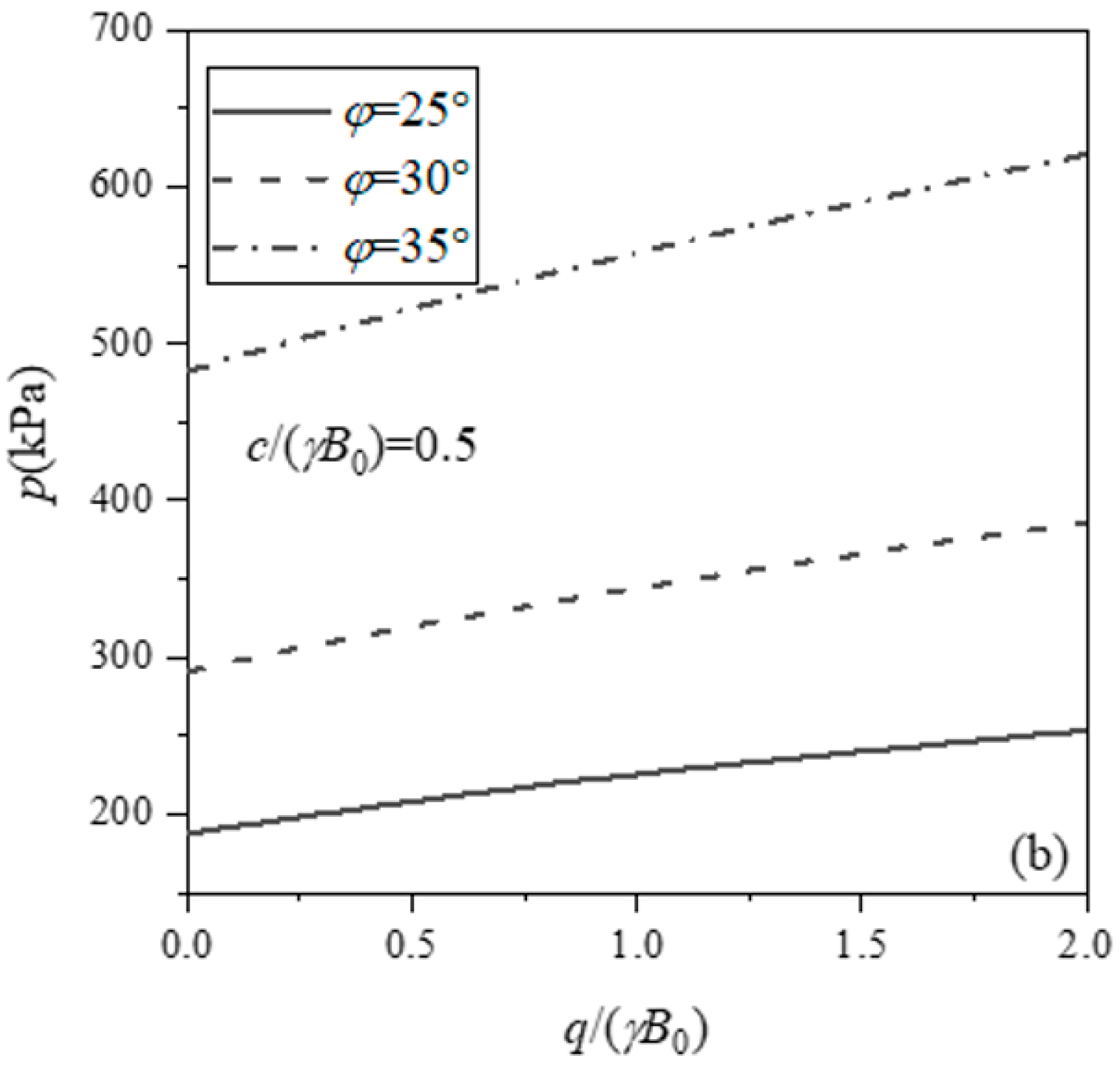
Figure 8 also shows the results of the seismic bearing capacity under four different combinations of and . It can be found that the uniform load and the cohesion have a significant effect on the bearing capacity. Therefore, in order to visualize the effect, the variation curves of the bearing capacity with the uniform load as well as the cohesion are given in Figure 8 and Figure 9, respectively.
Figure 9.
The trend of with at different . (a) ; (b) .
Figure 9 shows the variation in bearing capacity with at different . For Figure 9a, increases by about 120% when is increased from 0 to 2 for , whereas increases by about 70% when is increased from 0 to 2 for . For Figure 9b, increases by about 35% when is increased from 0 to 2 when , whereas increases by about 28% when is increased from 0 to 2 for . Furthermore, it is noticed that the slope of curve increases slightly as increases.
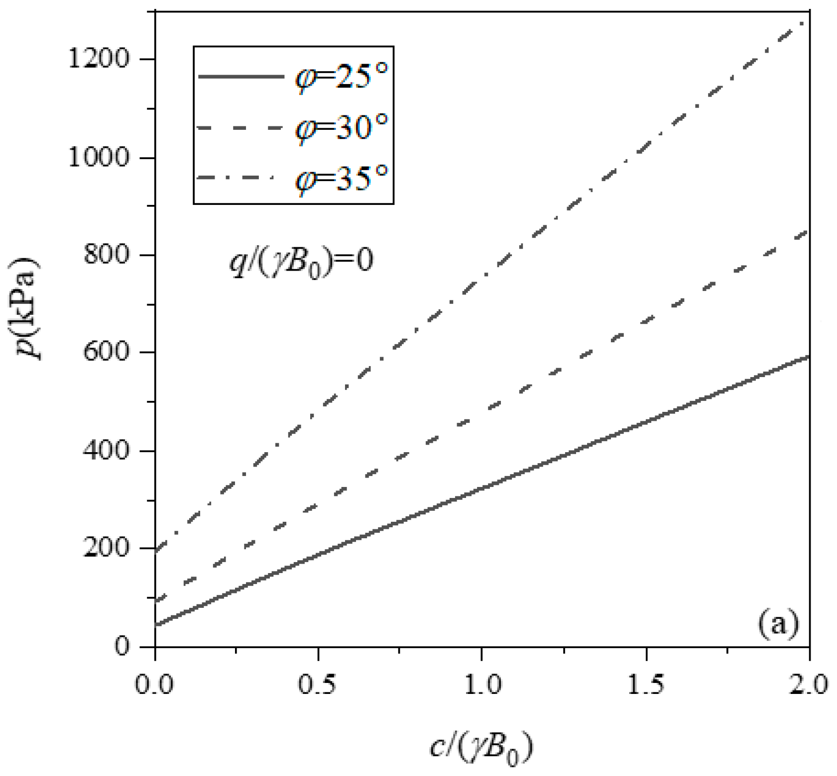
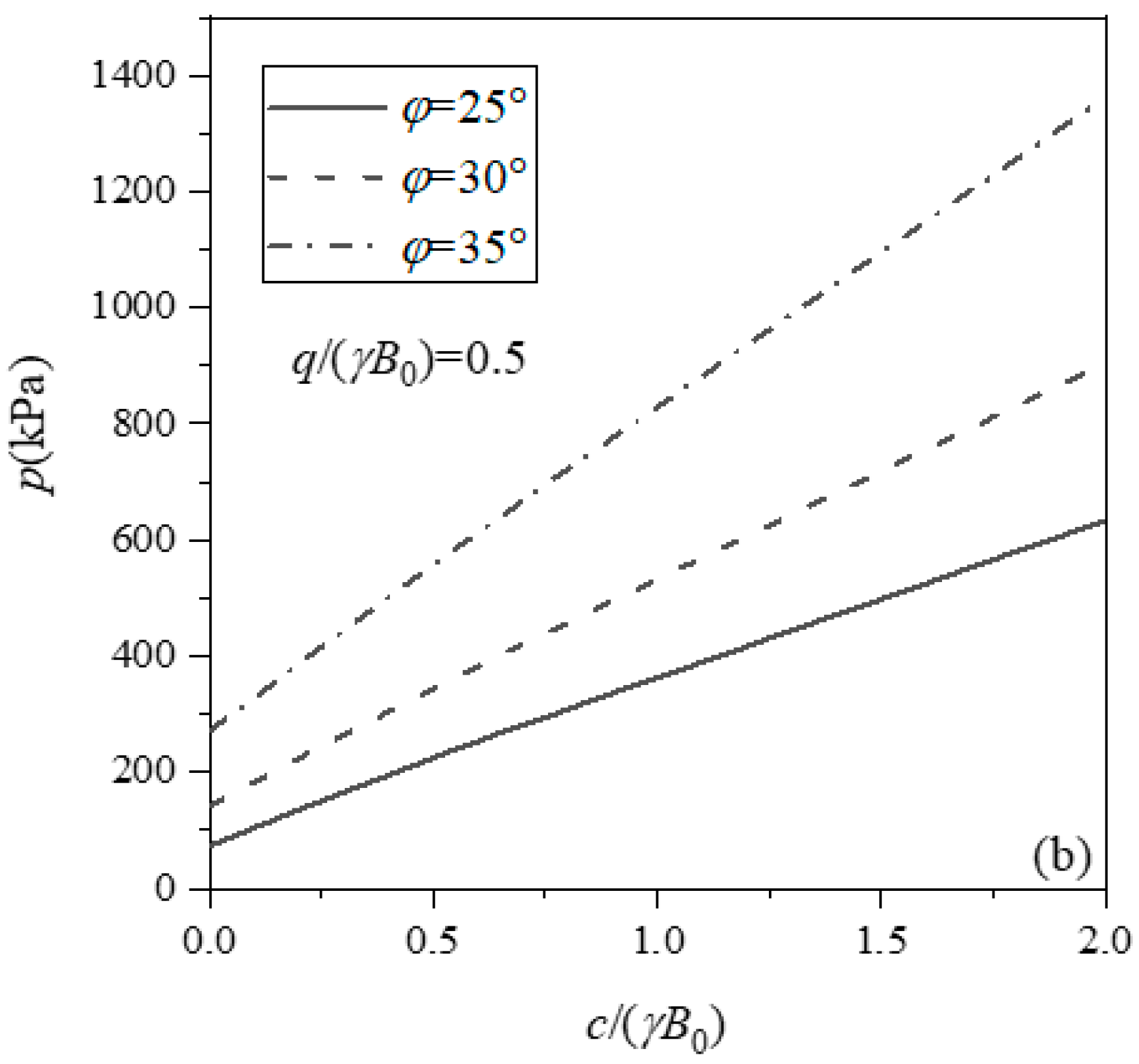
Figure 10 illustrates the variation in bearing capacity with for different . For Figure 10a, increases by about 1300% when increases from 0 to 2 for , whereas increases by about 570% for . For Figure 10b, increases by about 760% as increases from 0 to 2 when , and by about 400% for . The slope of the curve increases significantly with increasing . In conclusion, both and have a positive effect on the bearing capacity .
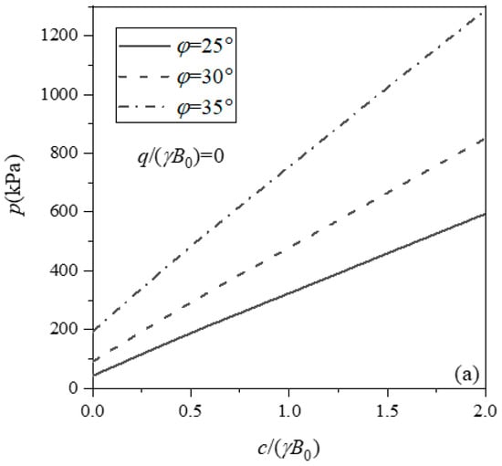
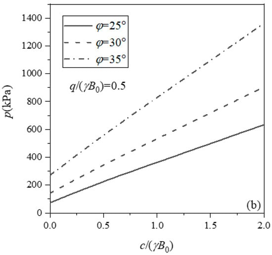
Figure 10.
The trend of with at different . (a) ; (b) .
4.3.3. Influence of and
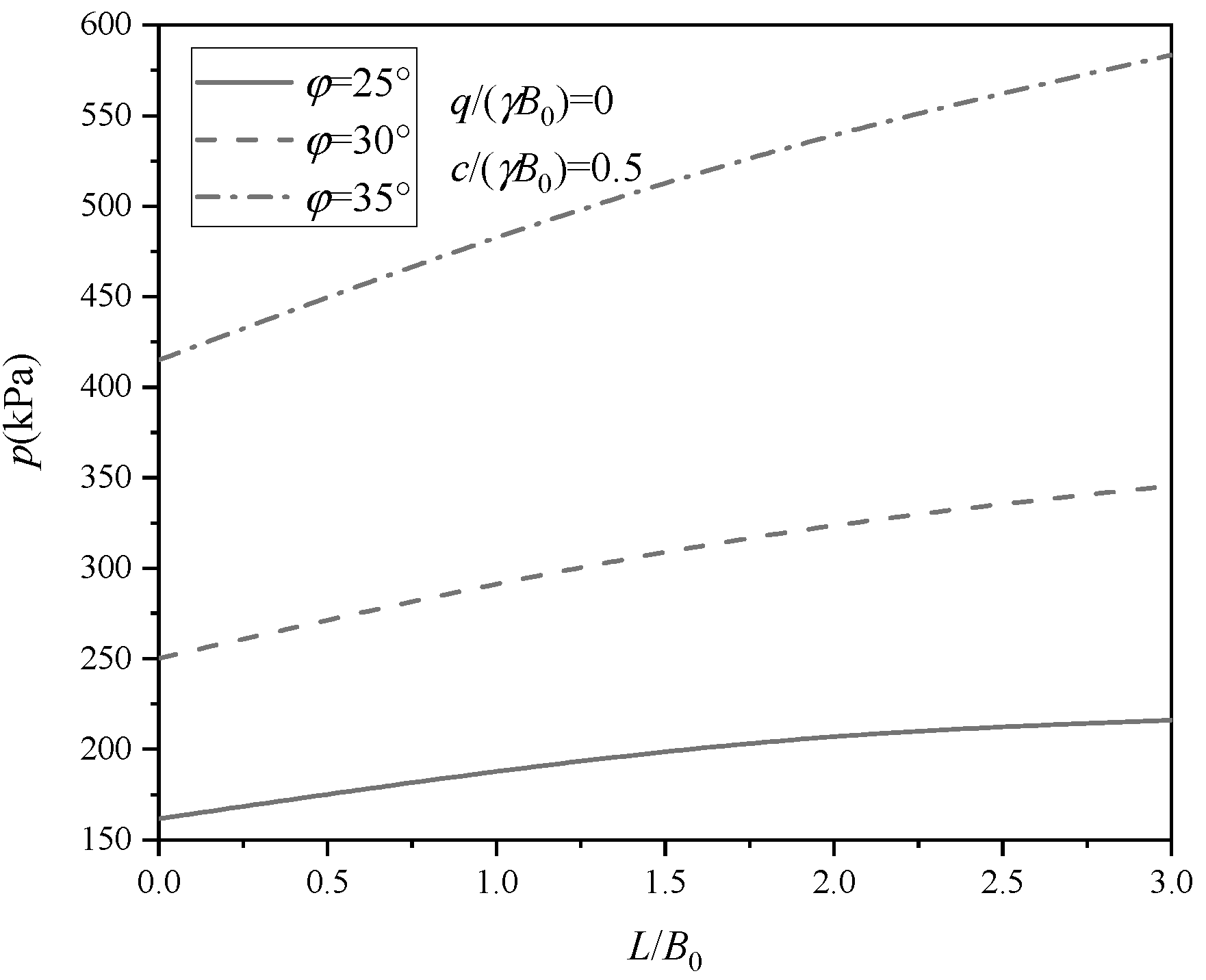
For adjacent-slope foundations, unlike foundations located on level ground, the bearing capacity is affected by the slope angle as well as the setback distance . Figure 11 illustrates the variation in seismic bearing capacity as a ratio of setback distance to foundation width for different . For , the bearing capacity increases by about 34% when increases from 0 to 3. In addition, it can be seen that there is a tendency for to converge slowly as increases. However, as increases, the convergence trend becomes less pronounced. Therefore, the further the foundation is from the slope surface apex, the higher its stability.

Figure 11.
The trend of with at different .
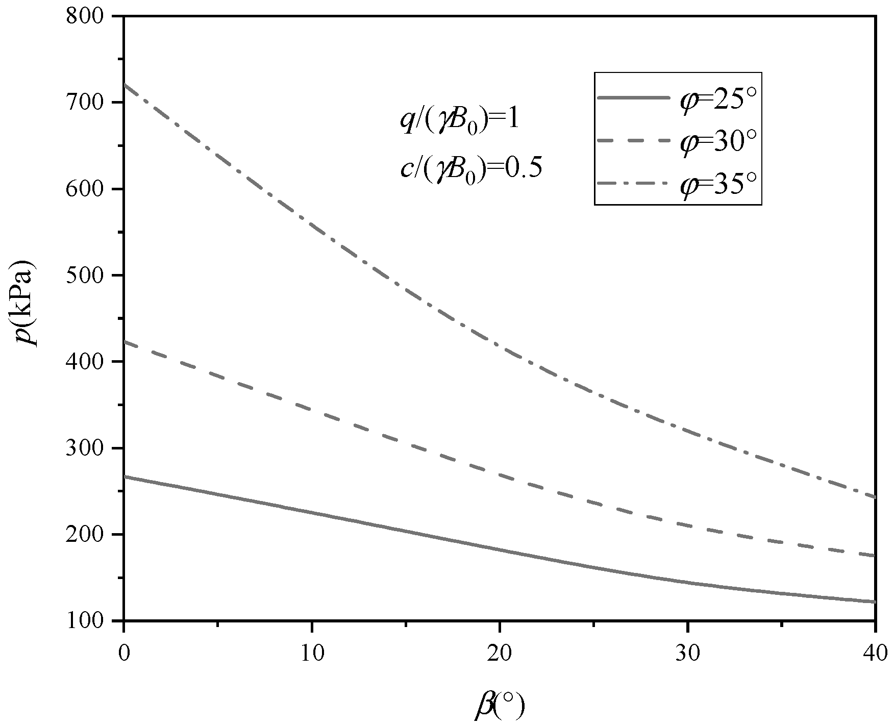
Figure 12 shows the trend of seismic bearing capacity with the slope angle for different . It is obvious that decreases as increases. For , the bearing capacity decreases by about 54% when increases from 0 to 40°. For , the bearing capacity reduces by about 66%. Therefore, the effect of slope angle on bearing capacity is significant, the steeper the slope, the lower the bearing capacity of the foundation located on it. In addition, the curves in Figure 12 also have a tendency to converge.

Figure 12.
The trend of with at different .
4.3.4. Influence of
In this subsection, the effect of non-uniformity of soil on seismic bearing capacity is investigated. As mentioned above, is the non-uniformity coefficient. The trend of foundation seismic bearing capacity with non-uniformity coefficient at different is given in Figure 13. increases with increase in . For , the bearing capacity raises by about 7% as increases from 0 to 1.4.
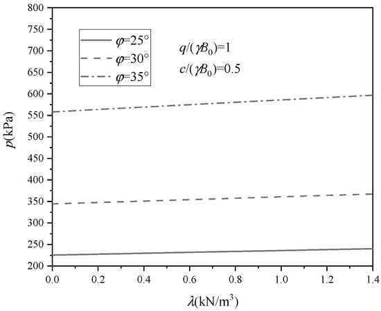
Figure 13.
The trend of with at different .
For , the bearing capacity also increases by about 7%. It can be seen that the non-uniformity of the soil will have certain influence on the bearing capacity, but in this paper, in order to simplify the calculation, the linear growth of the cohesion distribution model is selected, although this does not match with the reality, but shows the non-uniformity of the soil cannot be ignored.
4.3.5. Influence of and
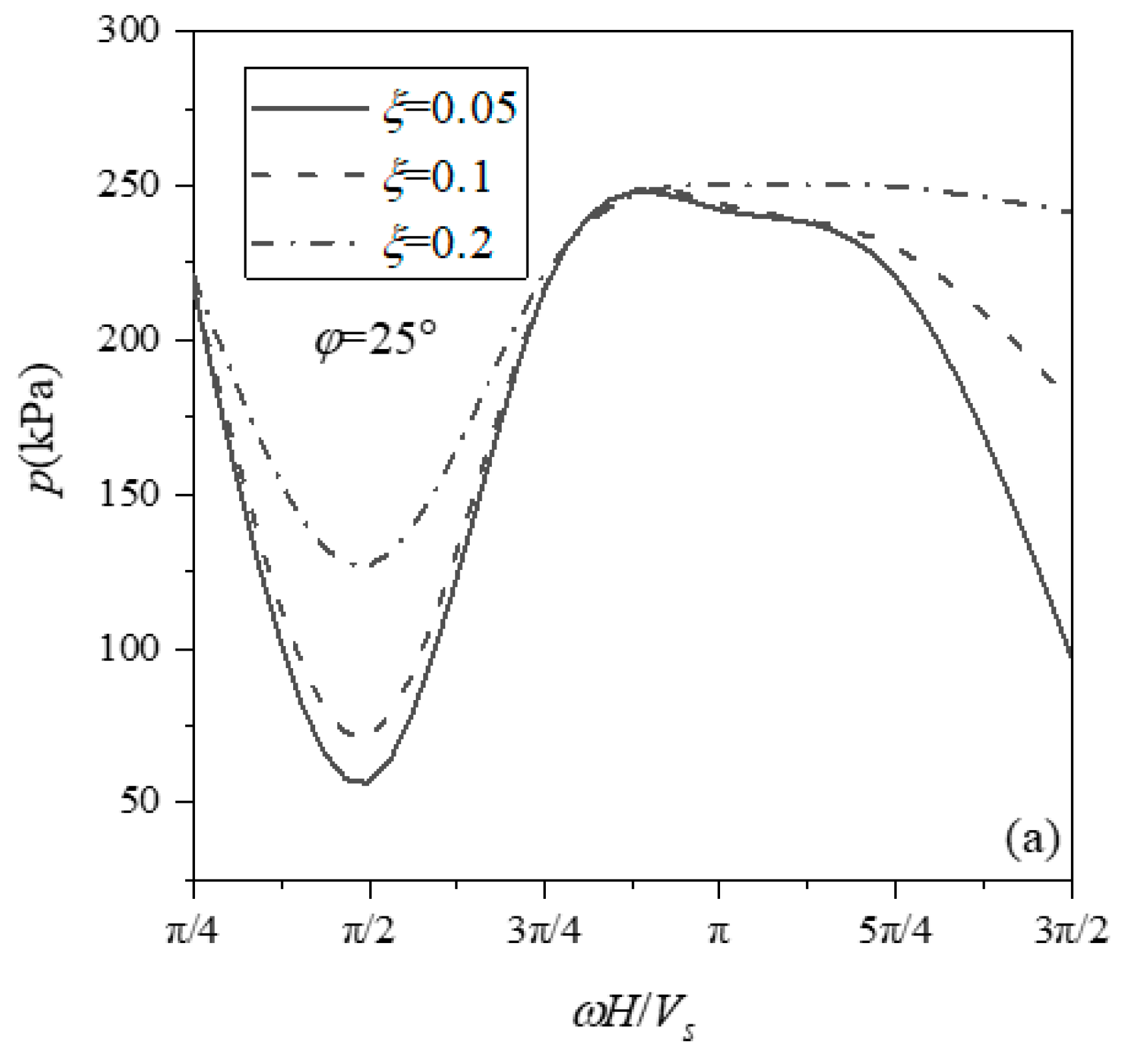
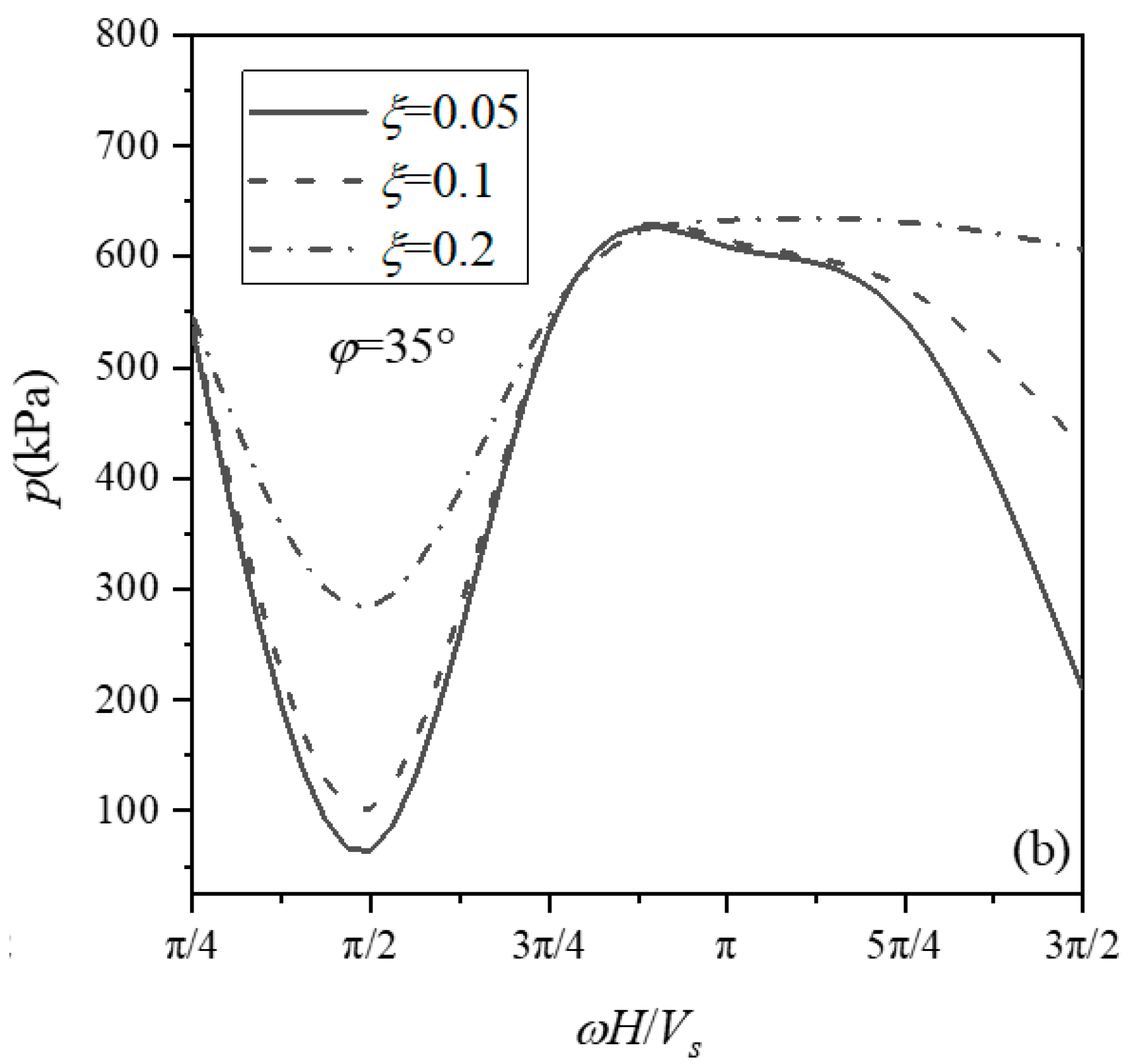
Figure 14 demonstrates the effect of normalized frequency and damping ratio on the seismic bearing capacity . There is a certain periodic pattern of the bearing capacity versus the normalized frequency , with a trough in the curve of the bearing capacity when and . For Figure 14a, when , the bearing capacity at is about 240% larger than that at . This indicates that for the seismic case, there is a most unfavorable situation for resonance to occur (). Moreover, for Figure 14a, when increases from 0.05 to 0.2 at , the bearing capacity increases by about 125%, whereas at , there is no significant change. Therefore, the effect of the damping ratio is different at different values of , and is most significant in the most unfavorable case.
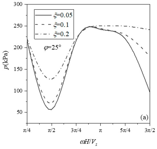
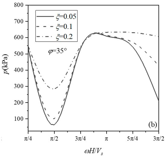
Figure 14.
The trend of with at different . (a) ; (b) .
5. Conclusions
This paper presents a framework for analyzing the seismic bearing capacity of foundations near slopes on non-uniform soils, considering the temporal and spatial characteristics of seismic forces. The modified pseudo-dynamic method is incorporated into the framework of the limit analysis upper bound method to obtain the formulation of the bearing capacity of the foundation near slope. Diverging from established pseudo-static and elementary pseudo-dynamic procedures, the advanced pseudo-dynamic formulation integrates the consideration of surface stress boundaries and damping ratio impacts, and more realistically reflects the spatial and temporal characteristics of seismic forces. The seismic forces are calculated using the more efficient layered superposition method. In addition, a linearly increasing cohesion model is used to characterize the non-uniformity of the soils. This paper compares and analyzes the calculated results with the existing literature and analyzes important parameters one by one. The main conclusions are as follows:
(1) The normalized frequency has a significant periodic effect on the seismic bearing capacity of foundations. When , the seismic bearing capacity will suddenly and abruptly decrease, and unfavorable working conditions occur, so special attention is needed in engineering practice.
(2) The effect of soil damping ratio on seismic capacity at is more significant, as the seismic bearing capacity increases with the increase in damping ratio. The effect of damping ratio at is minimum.
(3) The relationship between seismic bearing capacity and setback distance as well as slope angle has obvious convergence. As the setback distance grows, the structure’s seismic resistance improves, whereas steeper slope angles lead to reduced bearing capacity under earthquake conditions.
(4) The seismic bearing capacity is positively correlated with the initial cohesion and the non-uniformity coefficient, and the non-uniformity of the soils has a significant effect on the seismic bearing capacity.
This study investigates the bearing capacity of foundations adjacent to slopes under seismic conditions using a linear non-uniform soil profile, extending conventional homogeneous soil models to account for depth-dependent soil parameter variations. By integrating the upper bound theorem of limit analysis with the modified pseudo-dynamic method, the proposed framework addresses both slope proximity effects and seismic dynamics, providing practical references for engineering applications. The derived solutions demonstrate improved alignment with realistic bearing capacity behaviors compared to static or homogeneous soil assumptions.
The current methodology carries inherent limitations. The linear non-uniform soil profile represents an idealized simplification, as real stratigraphy often exhibits nonlinear heterogeneity. Theoretical prerequisites of the upper bound theorem (e.g., small deformation, elastic-plastic constitutive behavior) and modified pseudo-dynamic assumptions strictly govern all calculations. Furthermore, the adoption of linear failure criteria overlooks soil nonlinearity, while unsaturated soil mechanics and seepage effects remain unaddressed. These aspects warrant future refinement.
The results of this study exhibit broad applicability, with the model being validated for foundation bearing capacity analysis under seismic conditions while accounting for soil heterogeneity and slope proximity. However, the proposed framework is not applicable to unsaturated soil conditions or scenarios involving seepage effects.
This paper aims to study the seismic bearing capacity of the foundation near the slope on non-uniform soil, providing reference for practical engineering. However, there are some limitations in this paper. To simplify the calculation, the linear increasing cohesion model is used to characterize the non-uniformity of the soil. Consequently, more sophisticated modeling approaches could be integrated in subsequent research endeavors. Furthermore, the current investigation’s scope could be expanded to encompass unsaturated soil conditions and nonlinear soil failure mechanisms.
Author Contributions
Validation, formal analysis, writing-original draft, methodology, J.X.; investigation, supervision, D.Z.; resources, project administration, H.L.; visualization, project administration, date curation, supervision, J.Z. All authors have read and agreed to the published version of the manuscript.
Funding
This research received no external funding.
Institutional Review Board Statement
Not applicable.
Informed Consent Statement
Not applicable.
Data Availability Statement
The data analyzed are available from the corresponding author on reasonable request. The data are not publicly available due to reasons of privacy.
Conflicts of Interest
The authors declare no conflict of interest.
Appendix A
| means the seismic acceleration | |
| means the width of foundation | |
| means the height of the jth layer portion of the ith block | |
| means the cohesion of the soil | |
| means the length of the friction surface between the block and the undamaged soil | |
| means the work done by the internal forces | |
| means the volumetric force exerted on the soil | |
| means the amplification factor | |
| means the height of the retaining wall or the depth from bedrock | |
| means | |
| means | |
| means the coefficient of the seismic acceleration | |
| means the setback distance | |
| means the length of the contact surface of the blocks | |
| means the number of layers per block | |
| and | both are constants |
| means the bearing capacity factor related to cohesion | |
| means the bearing capacity factor related to soil unit weight | |
| means the width of the jth layer portion of the ith block | |
| means the work done by the surface loads. | |
| means the capacity of the foundation | |
| means the surface loads the foundation side | |
| means the area of the block | |
| means the area of the jth layer portion of the ith block | |
| means the surface force exerted on the soil | |
| means time | |
| means the thickness of the jth layer portion of the ith block | |
| are the wave velocities of shear and pressure waves | |
| means the velocity of the block | |
| means the work done by the external forces | |
| means the frequency | |
| means the depth of a certain point | |
| means the depth of the jth layer portion of the ith block | |
| means the top angle of the block | |
| means the bottom angle of the block | |
| means the angle of the slope | |
| means the soil unit weight | |
| means the plastic strain rate | |
| means nonlinearity coefficient | |
| means the wavelength | |
| means the damping ration of soils | |
| means the stress tensor | |
| means the angle between speed of block and vertical direction | |
| means the internal friction angle |
References
- Soubra, A.H. Upper-bound solutions for bearing capacity of foundations. J. Geotech. Geoenviron. Eng. 1999, 125, 59–68. [Google Scholar] [CrossRef]
- Saada, Z.; Maghous, S.; Garnier, D. Seismic bearing capacity of shallow foundations near rock slopes using the generalized Hoek-Brown criterion. Int. J. Numer. Anal. Methods Geomech. 2011, 35, 724–748. [Google Scholar] [CrossRef]
- Raj, D.; Singh, Y.; Shukla, S.K. Seismic Bearing Capacity of Strip Foundation Embedded in c-ϕ Soil Slope. Int. J. Geomech. 2018, 18, 04018076. [Google Scholar] [CrossRef]
- Wu, G.; Zhao, M.; Zhang, R.; Lei, M. Ultimate Bearing Capacity of Strip Footings on Hoek–Brown Rock Slopes Using Adaptive Finite Element Limit Analysis. Rock Mech. Rock Eng. 2021, 54, 1621–1628. [Google Scholar] [CrossRef]
- Wu, G.; Zhao, H.; Zhao, M.; Duan, L. Ultimate bearing capacity of strip footings lying on Hoek–Brown slopes subjected to eccentric load. Acta Geotech. 2023, 18, 1111–1124. [Google Scholar] [CrossRef]
- Keshavarz, A.; Kumar, J. Bearing Capacity of Foundations over Rock Slopes–Slip Lines and FELA Solutions. Int. J. Geomech. 2024, 24, 04024229. [Google Scholar] [CrossRef]
- Steedman, R.S.; Zeng, X. The influence of phase on the calculation of pseudo-static earth pressure on a retaining wall. Géotechnique 1990, 40, 103–112. [Google Scholar] [CrossRef]
- Choudhury, D.; Nimbalkar, S.S. Pseudo-dynamic approach of seismic active earth pressure behind retaining wall. Geotech. Geol. Eng. 2006, 24, 1103–1113. [Google Scholar] [CrossRef]
- Ghosh, S. Pseudo-dynamic active force and pressure behind battered retaining wall supporting inclined backfill. Soil Dyn. Earthq. Eng. 2010, 30, 1226–1232. [Google Scholar] [CrossRef]
- Bellezza, I.; D’Alberto, D.; Fentini, R. Pseudo-dynamic approach for active thrust of submerged soils. Proc. Inst. Civ. Engineers. Geotech. Eng. 2012, 165, 321–333. [Google Scholar] [CrossRef]
- Bellezza, I. A New Pseudo-dynamic Approach for Seismic Active Soil Thrust. Geotech. Geol. Eng. 2014, 32, 561–576. [Google Scholar] [CrossRef]
- Wei, L.; Xu, Q.; Wang, S.; Ji, X. The primary influence of shear band evolution on the slope bearing capacity. J. Rock Mech. Geotech. Eng. 2023, 15, 1023–1037. [Google Scholar] [CrossRef]
- Kang, X.D.; Yang, X.L.; Wu, C.G. Modified pseudo-dynamic bearing capacity of reinforced soil foundations. Comput. Geotech. 2024, 165, 105901. [Google Scholar] [CrossRef]
- Tan, M.; Vanapalli, S.K. Foundation bearing capacity estimation on unsaturated soil slope under transient flow condition using slip line method. Comput. Geotech. 2022, 148, 104804. [Google Scholar] [CrossRef]
- Kumar, J.; Korada, V.S. Seismic bearing capacity factor Nγ for a rough strip footing on sloping ground. Comput. Geotech. 2022, 153, 105054. [Google Scholar] [CrossRef]
- Peng, W.; Zhao, M.; Zhao, H.; Yang, C. Effect of slope on bearing capacity of laterally loaded pile based on asymmetric failure mode. Comput. Geotech. 2021, 140, 104469. [Google Scholar] [CrossRef]
- Yang, X.L.; Yin, J.H. Slope stability analysis with nonlinear failure criterion. J. Eng. Mech. 2004, 130, 267–273. [Google Scholar] [CrossRef]
- Al-Shamrani, M.A. Upper-bound solutions for bearing capacity of strip footings over anisotropic nonhomogeneous clays. Soils Found. 2005, 45, 109–124. [Google Scholar] [CrossRef]
- Nian, T.K.; Chen, G.Q.; Luan, M.T.; Yang, Q.; Zheng, D.F. Limit analysis of the stability of slopes reinforced with piles against landslide in nonhomogeneous and anisotropic soils. Can. Geotech. J. 2008, 45, 1092–1103. [Google Scholar] [CrossRef]
- Han, C.; Chen, J.; Xia, X.; Wang, J. Three-dimensional stability analysis of anisotropic and non-homogeneous slopes using limit analysis. J. Cent. South Univ. 2014, 21, 1142–1147. [Google Scholar] [CrossRef]
- Hou, C.; Zhang, T.; Sun, Z.; Dias, D.; Shang, M. Seismic Analysis of Nonhomogeneous Slopes with Cracks Using a Discretization Kinematic Approach. Int. J. Geomech. 2019, 19. [Google Scholar] [CrossRef]
- Kang, X.D.; Zhu, J.Q.; Liu, L.L. Seismic Bearing Capacity of Strip Footings with Modified Pseudo-dynamic Method. KSCE J. Civ. Eng. 2024, 28, 1657–1674. [Google Scholar] [CrossRef]
- Yang, X.L.; Yin, J.H. Upper bound solution for ultimate bearing capacity with a modified Hoek-Brown failure criterion. Int. J. Rock Mech. Min. Sci. 2005, 42, 550–560. [Google Scholar] [CrossRef]
- Osman, A.S. Upper bound solutions for the shape factors of smooth rectangular footings on frictional materials. Comput. Geotech. 2019, 115, 103177. [Google Scholar] [CrossRef]
- Kang, X.D.; Zhu, J.Q.; Yang, X.L. Seismic bearing capacity of rock foundations subjected to seepage by a unilateral piece-wise log-spiral failure mechanism. Comput. Geotech. 2023, 158, 105363. [Google Scholar] [CrossRef]
- Shan, J.T.; Wu, Y.M.; Yang, X.L. Three-dimensional stability of two-step slope with crack considering temperature effect on unsaturated soil. J. Cent. South Univ. 2025, 32, 1–19. [Google Scholar] [CrossRef]
- Yang, X.L.; Li, L.; Yin, J.H. Seismic and static stability analysis for rock slopes by a kinematical approach. Geotechnique 2004, 54, 543–549. [Google Scholar] [CrossRef]
- Liao, H.; Xu, S.; Wu, C.G. 3D seismic bearing capacity of rectangular foundations near rock slopes using upper bound method. Alex. Eng. J. 2024, 109, 778–791. [Google Scholar] [CrossRef]
- Manna, D.; Santhoshkumar, G.; Ghosh, P. Upper-bound limit load of rigid pavements resting on reinforced soil embankments—Kinematic approach. Transp. Geotech. 2021, 30, 100611. [Google Scholar] [CrossRef]
- Sawada, T.; Nomachi, S.G.; Chen, W.F. Seismic bearing capacity of a mounded foundation near a down-hill slope by pseudo-static analysis. Soils Found. 1994, 34, 11–17. [Google Scholar] [CrossRef]
- Askari, F.; Farzaneh, O. Upper-bound solution for seismic bearing capacity of shallow foundations near slopes. Géotechnique 2003, 53, 697–702. [Google Scholar] [CrossRef]
- Ghosh, P.; Kumar, J. Seismic bearing capacity of strip footings adjacent to slopes using the upper bound limit analysis. Electron. J. Geotech. Eng. 2005, 10, 1–13. [Google Scholar]
- Soufi, G.R.; Chenari, R.J.; Javankhoshdel, S. Conventional vs. modified pseudo-dynamic seismic analyses in the shallow strip footing bearing capacity problem. Earthq. Eng. Eng. Vib. 2021, 20, 993–1006. [Google Scholar] [CrossRef]
- Zhong, J.H.; Li, Y.X.; Yang, X.L. Estimation of the Seismic Bearing Capacity of Shallow Strip Footings Based on a Pseudodynamic Approach. Int. J. Geomech. 2022, 22, 04022143. [Google Scholar] [CrossRef]

Disclaimer/Publisher’s Note: The statements, opinions and data contained in all publications are solely those of the individual author(s) and contributor(s) and not of MDPI and/or the editor(s). MDPI and/or the editor(s) disclaim responsibility for any injury to people or property resulting from any ideas, methods, instructions or products referred to in the content. |
© 2025 by the authors. Licensee MDPI, Basel, Switzerland. This article is an open access article distributed under the terms and conditions of the Creative Commons Attribution (CC BY) license (https://creativecommons.org/licenses/by/4.0/).