Influence of Source Shape on Semi-Airborne Transient Electromagnetic Surveys

Abstract

The semi-airborne transient electromagnetic (SATEM) method has garnered increasing attention and research interest due to its superior detection depth and high efficiency. Theoretically, the SATEM method employs a long straight grounded wire as its transmitter source; however, in practical applications, various source shapes emerge due to terrain constraints. This paper investigates the influence of source shape on SATEM data. A three-dimensional (3D) block model is established, and a model order reduction algorithm is applied to calculate the 3D spatial distribution of electromagnetic fields generated by both an ideal linear source and a curved source. Numerical simulation results reveal that: (1) in the early stage, maximum values of electric and magnetic fields near the source are distributed along the source shape; this influence diminishes with time, and at the late stage, the spatial electromagnetic field distributions generated by linear and curved sources converge, exhibiting similar patterns regardless of the source geometry; (2) the source shape primarily affects early responses in small-offset areas while having minimal influence on late responses in large-offset regions; (3) for deep detection applications conducted in large-offset areas, the influence of the source shape can be disregarded; however, for shallow detection with receivers positioned in small-offset regions, the source shape effects should be taken into consideration.

1. Introduction

In recent years, the semi-airborne transient electromagnetic (SATEM) method has garnered significant attention and undergone substantial development [1,2,3,4,5,6]. It has been successfully applied in various fields, including deep sulfide deposit exploration [7,8], graphite exploration [9], iron ore exploration [10], underwater geological mapping [11], coal seam gob exploration [12], and tunnel geological risk investigation [13]. This innovative approach utilizes a high-power ground-based wire source to transmit magnetic field signals while employing helicopters or unmanned aerial vehicles to receive magnetic field signals in the air, enabling rapid surface scanning and data acquisition [12]. Compared to conventional airborne electromagnetic methods, the SATEM technique offers greater detection depth and penetration capabilities [6]. Furthermore, when contrasted with traditional ground-based electromagnetic methods, SATEM demonstrates superior operational efficiency and versatility, making it especially valuable for investigating geologically complex and topographically challenging regions [14]. The method’s hybrid nature—combining ground-based transmitters with airborne receivers—creates an optimal balance between detection depth, survey speed, and adaptability to difficult terrain [6,14].

In theory, the SATEM method employs a long straight wire grounded at both ends to form a closed circuit with the earth. A stable current flows through this wire, generating a consistent primary magnetic field. When the current is abruptly terminated, eddy currents are induced in subsurface conductive bodies, which subsequently generate secondary magnetic fields [15]. The temporal variations in these secondary magnetic fields are then measured by receivers mounted on airborne platforms. In practical field operations, however, the ideal linear configuration of the transmitter wire is often compromised by topographical constraints and accessibility issues. Consequently, the wire must conform to available terrain features or follow existing roads, resulting in irregular geometric configurations rather than the theoretical straight-line arrangement. These deviations from the ideal model significantly alter the underground induced current distribution patterns and, by extension, the characteristics of the secondary magnetic fields. If data interpretation continues to rely on algorithms developed for straight-wire source models, the accuracy of geological interpretations may be substantially compromised. Therefore, comprehensive consideration of the transmitter wire geometry and its influence on electromagnetic field observations becomes crucial for accurate interpretations of SATEM survey data.

Extensive research has been conducted to investigate the influence of the source geometry on electromagnetic field measurements. Streich and Becken [16] examined the discrepancies between frequency-domain electromagnetic fields generated by finite-length wire sources versus point dipoles. Their findings revealed that these differences can be substantial over distances extending to several times the wire length. Chen et al. [17] investigated the impact of the transient electromagnetic source geometry on measurement outcomes with a one-dimensional (1D) model. The results demonstrated that the source geometry effects exceed 10% at small transmitter–receiver offsets, with a diminishing influence as the offset increases. Li et al. [18] conducted a comparative analysis of linear and arcuate sources with transient electromagnetic observation of equatorial and axial 1D models. The results show that the influence of the equatorial electric and magnetic field gradually increases with the decrease in the offset. Zhou et al. [19] further explored source geometry effects on short-offset transient electromagnetic measurements. Their research established an inverse relationship between subsurface resistivity and the relative difference in electric field responses between straight and distorted source geometries. Zhou et al. [20] calculated frequency-domain electromagnetic responses for several typical source configurations, concluding that the source geometry exerts greater influence on frequency-domain electric fields compared to magnetic fields. Nazari et al. [21] investigated the impact of various acquisition parameters on three-dimensional (3D) inversion outcomes for SATEM data. Their results emphasized the importance of source length.

Current research on source geometry effects has predominantly relied on 1D simplified models, with analyses focusing primarily on electromagnetic responses along with the 1D receiver profiles or inversion results derived therefrom. There remains a significant research gap regarding comprehensive 3D modeling approaches and the spatial distribution of electromagnetic fields in complex geological environments. Building upon the groundbreaking work of Gunderson et al. [15] on grounded source configurations, this study establishes a representative 3D SATEM survey model to address this knowledge deficit. We implement an advanced 3D modeling algorithm [22] based on finite volume spatial discretization [23] and model order reduction [24] techniques to compute the comprehensive distribution of electric and magnetic fields generated by both linear and curvilinear source geometries. Through systematic comparative analysis, this paper provides a comprehensive assessment of source geometry influences on SATEM survey outcomes in realistic 3D contexts.

2. Methods

To systematically investigate the influence of the source geometry on SATEM measurements, comprehensive forward modeling approaches incorporating both 1D and 3D frameworks are essential. In this study, we implement the 1D modeling methodology developed by Zhang et al. [25], which efficiently handles layered earth structures while accounting for source geometry variations. For more complex geological scenarios requiring full 3D representation, we employ the advanced computational framework proposed by Liu et al. [22], which integrates finite volume spatial discretization with model order reduction techniques to achieve computationally efficient yet accurate 3D electromagnetic field simulations. This dual modeling approach enables the rigorous quantification of source geometry effects across varying levels of geological complexity and provides a robust foundation for subsequent analysis.

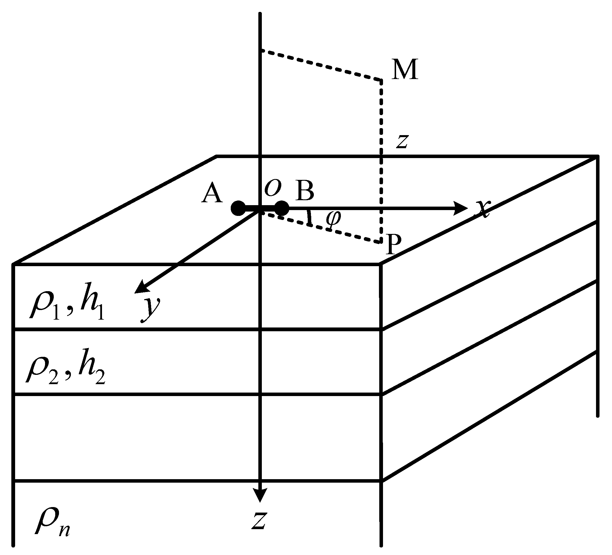
2.1. SATEM 1D Modeling

We establish a stratified n-layer earth model characterized by resistivity and thickness parameters denoted as ${\rho }_1,h_1;{\rho }_2,h_2;\dots ;{\rho }_n,h_n$, where $h_n\to \infty$ represents the semi-infinite bottom layer. An electric dipole source AB is positioned on the earth’s surface and oriented along the positive X-axis direction. The coordinate system is defined such that the origin O coincides with the center of the electric dipole. For any arbitrary measurement point M situated in the air, we define z as its vertical distance from the earth’s surface. The horizontal distance between the surface projection point P of measurement point M and the coordinate origin O is denoted as r, while φ represents the azimuthal angle between vector r and the positive X-axis direction. This geometric configuration is illustrated comprehensively in Figure 1.

In practical field applications, long wire sources typically extend for several kilometers, rendering the conventional electric dipole approximation inadequate in near-field and transition zones. To address this limitation, we implement a superposition principle wherein the extended source is discretized into m infinitesimal dipole elements, each with length ds. The electromagnetic field contribution from each elemental dipole is then systematically integrated to accurately reconstruct the composite field generated by the entire source configuration. Employing vector and scalar potential formalism as described by Zhang et al. [25], the frequency-domain magnetic induction intensity generated by an extended wire source can be mathematically expressed as

$$\left\{\begin{array}{c}{B}_x(\omega )={\sum }_{j=1}^m\left[\begin{array}{c}-{\displaystyle \frac{P_{Ej}}{2\pi }}{\displaystyle \frac{{\mu }_0\mathit{sin}{\phi }_j\mathit{cos}{\phi }_j}{r_j}}{\int }_0^{\infty }{\displaystyle \frac{2\lambda }{\lambda +\frac{u_1}{R_1}}}{e}^{\lambda z}{J}_1(\lambda r_j)d\lambda \\ +{\displaystyle \frac{P_{Ej}}{2\pi }}{\mu }_0\mathit{sin}{\phi }_j\mathit{cos}{\phi }_j{\int }_0^{\infty }{\displaystyle \frac{{\lambda }^2}{\lambda +\frac{u_1}{R_1}}}{e}^{\lambda z}{J}_0(\lambda r_j)d\lambda \end{array}\right]\hspace{1em}\hspace{1em}\\ B_y(\omega )={\sum }_{j=1}^m\left[\begin{array}{c}{\displaystyle \frac{P_{Ej}}{2\pi }}{\displaystyle \frac{{\mu }_0({\mathit{cos}}^2{\phi }_j-{\mathit{sin}}^2{\phi }_j)}{r_j}}{\int }_0^{\infty }{\displaystyle \frac{\lambda }{\lambda +\frac{u_1}{R_1}}}{e}^{\lambda z}{J}_1(\lambda r_j)d\lambda \\ +{\displaystyle \frac{P_{Ej}}{2\pi }}{\mu }_0{\mathit{sin}}^2{\phi }_j{\int }_0^{\infty }{\displaystyle \frac{{\lambda }^2}{\lambda +\frac{u_1}{R_1}}}{e}^{\lambda z}{J}_0(\lambda r_j)d\lambda \hspace{1em}\hspace{1em}\hspace{1em}\hspace{1em}\end{array}\right]\\ B_z(\omega )={\sum }_{j=1}^m{\displaystyle \frac{P_{E_j}}{2\pi }}{\mu }_0\mathit{sin}{\phi }_j{\int }_0^{\infty }{\displaystyle \frac{{\lambda }^2}{\lambda +\frac{u_1}{R_1}}}{e}^{\lambda z}{J}_1(\lambda r_j)d\lambda \hspace{1em}\hspace{1em}\hspace{1em}\hspace{1em}\hspace{1em}\hspace{1em}\end{array}\right.$$

(1)

where $R_1=cth\left[u_1{h}_1+arcth{\displaystyle \frac{u_1}{u_2}}cth(u_2{h}_2+...+arcth{\displaystyle \frac{u_{n-1}}{u_n}})\right]$, and $u_i=\sqrt{{\lambda }^2-i\omega \mu /{\rho }_i}$. The parameter $P_{E_j}=Id{s}_j$ represents the dipole moment of the j discretized element, with $I$ denoting the current intensity and ${ds}_j$ representing the length of the j electric dipole segment. The geometric parameters ${\phi }_j$ and $r_j$ correspond to the azimuthal angle between the projection point P and the j electric dipole segment and the horizontal offset distance, respectively. The variable m denotes the total number of discretized segments comprising the extended electrical source.

For step-function excitation, the time-domain SATEM responses $B\left(t\right)$ and $dB\left(t\right)/dt$ can be derived from the frequency-domain response $B\left(\omega \right)$ through the following integral transformation relations as established by Zhang et al. [25]:

$$\left\{\begin{array}{c}B\left(t\right)={\displaystyle \frac{2}{\pi }}{\int }_0^{\mathrm{\infty }}{\displaystyle \frac{\mathrm{R}\mathrm{e}\left[B\left(\omega \right)\right]}{\omega }}\mathrm{s}\mathrm{i}\mathrm{n}\left(\omega t\right)d\omega \\ {\displaystyle \frac{\partial B\left(t\right)}{\partial t}}=-{\displaystyle \frac{2}{\pi }}{\int }_0^{\mathrm{\infty }}\mathrm{R}\mathrm{e}\left[B\left(\omega \right)\right]\mathrm{c}\mathrm{o}\mathrm{s}(\omega t)d\omega \end{array}\right.$$

(2)

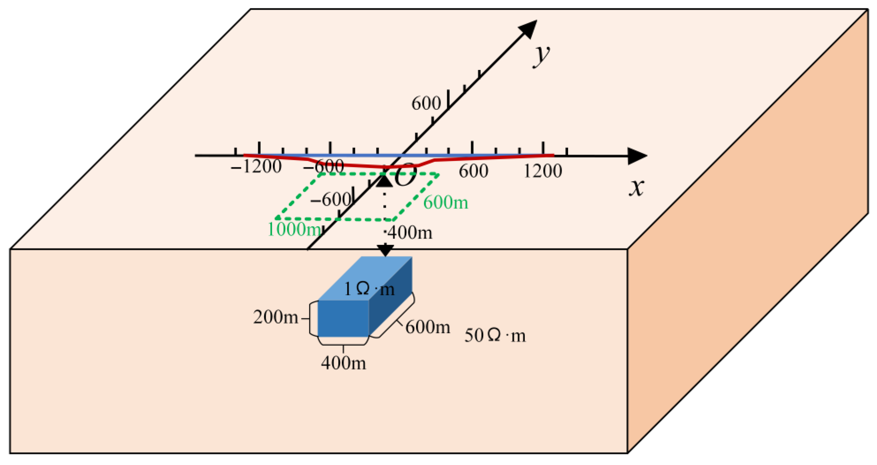
2.2. SATEM 3D Modeling

The 3D numerical simulation of SATEM is implemented through finite volume spatial discretization coupled with model order reduction techniques for efficient time-domain solutions. The governing Maxwell’s equations in the time domain applicable to the SATEM configuration can be expressed as [22]

$$\left\{\begin{array}{c}{\displaystyle \frac{\partial \overrightarrow{B}}{\partial t}}=-\nabla \times \overrightarrow{E} \\ \nabla \times {\mu }^{-1}\overrightarrow{B}-\sigma \overrightarrow{E}=\overrightarrow{s}\end{array}\right.$$

(3)

where $\overrightarrow{E}$ denotes the electric field intensity vector (V/m), $\overrightarrow{B}$ represents the magnetic flux density vector (T), $t$ is the time variable (s), $\mu$ is the magnetic permeability (H/m), $\sigma$ corresponds to the electrical conductivity (S/m), and $\overrightarrow{s}$ designates the external source current density term (A/m²). The system is subject to natural boundary conditions as described by Haber [23]:

$$\overrightarrow{B}\times \overrightarrow{n}=0;\overrightarrow{n}\times \overrightarrow{E}=0$$

(4)

The governing Equation (3) is spatially discretized using the finite volume method implemented on a structured hexahedral mesh. The discretization process yields the following semi-discrete system:

$$\left\{\begin{array}{c}{\displaystyle \frac{\partial \mathbf{b}}{\partial t}}+\mathrm{C}\mathrm{U}\mathrm{R}\mathrm{L}\mathbf{e}=0 \\ {\mathrm{C}\mathrm{U}\mathrm{R}\mathrm{L}}^{\mathrm{T}}{\mathbf{M}}_{f\mu }\mathbf{b}-{\mathbf{M}}_{e\sigma }\mathbf{e}={\mathbf{M}}_e\mathbf{s}\end{array}\right.$$

(5)

where $\mathbf{e}$ and $\mathbf{b}$ represent the orthogonal projections of the electric field vector $\overrightarrow{E}$ and magnetic flux density vector $\overrightarrow{B}$ onto the edges and face centers of the computational grid elements, respectively. $\mathrm{C}\mathrm{U}\mathrm{R}\mathrm{L}$ denotes the discrete curl operator matrix derived from the spatial discretization scheme. The matrices ${\mathbf{M}}_{f\mu }$ and ${\mathbf{M}}_{e\sigma }$ are the mass matrices incorporating the magnetic permeability $\mu$ and electrical conductivity $\sigma$ distributions within the computational domain. For step-function excitation, the electric field can be eliminated from the system, resulting in the following discrete governing equation for the magnetic flux density:

$${\displaystyle \frac{\partial \mathbf{b}}{\partial t}}=\mathbf{A}\mathbf{b}$$

(6)

where $\mathbf{A}=-\mathrm{C}\mathrm{U}\mathrm{R}\mathrm{L}{\mathbf{M}}_{e\sigma }^{-1}{\mathrm{C}\mathrm{U}\mathrm{R}\mathrm{L}}^{\mathrm{T}}{\mathbf{M}}_{f\mu }$. The magnetic field at the time $t$ obtained by Equation (6) is a matrix exponential function:

$${\mathbf{b}}^t=\mathrm{e}\mathrm{x}\mathrm{p}\left(t\mathbf{A}\right){\mathbf{b}}^0$$

(7)

where ${\mathbf{b}}^0$ denotes the initial magnetic flux density distribution at $t=0$. For a grounded long wire source configuration, the initial magnetic flux density corresponds to the solution of a magnetostatic problem, which can be obtained by applying the finite volume method to solve the steady-state Maxwell’s equations as described by Liu et al. [22]. Substituting this initial magnetic flux density into Equation (6) enables the computation of $\partial \mathbf{b}/\partial t$. Equation (7) is subsequently solved using the rational Krylov subspace method. Based on the system matrix $\mathbf{A}$ and the initial magnetic flux density vector ${\mathbf{b}}^0$, we construct the rational Krylov subspace $\kappa \left(\right(\mathbf{A}-{\xi }_i\mathbf{I}{)}^{-1},{\mathbf{b}}^0)$, where ${\xi }_i$ represents the shift parameters. The orthonormal basis ${\mathbf{V}}_{m+1}$ of this subspace and the projection matrix ${\mathbf{A}}_{m+1}={\mathbf{V}}_{m+1}^{\mathrm{T}}\mathbf{A}{\mathbf{V}}_{m+1}$ are then computed. Consequently, the model order reduction approximate solution of Equation (7) is expressed as

$$\mathbf{b}\approx {\mathbf{b}}_m={\mathbf{V}}_{m+1}\mathrm{e}\mathrm{x}\mathrm{p}(-t{\mathbf{A}}_{m+1})\left(∥{\mathbf{b}}^0∥{\mathbf{e}}_1\right)$$

(8)

where ${\mathbf{e}}_1$ is the first identity vector.

2.3. SATEM Model

To investigate the influence of the source geometry on SATEM responses, we established a numerical model with the transmitter–receiver configuration illustrated in Figure 2. The background medium consists of a homogeneous half-space with a resistivity of 50 Ω·m. A conductive 3D anomalous body with dimensions of 400 m × 600 m × 200 m and resistivity of 1 Ω·m is embedded at a depth of 400 m, positioned 500 m laterally from the source.

Two distinct transmitter configurations were examined: a straight-line source (depicted by the blue line) with a total length of 2.5 km and a curved source (depicted by the red line) with a total length of 2.8 km. Both sources share identical endpoint locations; however, the curved source incorporates a significant bend in its central section. The airborne receivers (shown in green) were positioned at an elevation of 20 m above the ground surface to measure the induced electromagnetic responses.

Initially, we computed the SATEM responses for the homogeneous 1D half-space model using different source configurations, without incorporating the conductive 3D anomalous body, to establish baseline responses. Then, we calculated the SATEM responses for the 3D model using sources with varying geometries, as illustrated in Figure 2. Subsequently, we conducted a comprehensive analysis to evaluate the influence of the source geometry on the observed electromagnetic data in this modeling scenario.

3. Results

3.1. Half-Space Model

3.1.1. Electric Fields in the Earth

To comprehend the magnetic field distribution characteristics, it is essential to first analyze the electric field distribution patterns. Figure 3 illustrates the electric field distribution on the surface (oxy plane) at different time instants for both linear and curved sources. Figure 3a–c represent the curved source responses, while Figure 3d–f depict the linear source responses.

When the transmitting current is abruptly terminated, induced currents concentrate in proximity to the wire to maintain spatial consistency in the magnetic field distribution, resulting in corresponding spatial patterns in the electric field. During the early transient stage, the electric field distributions in the immediate vicinity of the wire differ significantly between the two source geometries; however, the distributions in regions distant from the wire remain essentially identical, as demonstrated in Figure 3a,d. As the transient process evolves, the current begins to diffuse downward, diminishing the influence of the source geometry and reducing the disparities in electric field distributions near the wire, as illustrated in Figure 3b,e. In the late transient stage (t = 0.01 s), as shown in Figure 3c,f, the electric field distributions for both curved and linear sources become virtually indistinguishable.

Figure 4 presents the electric field distribution in the oyz plane intersecting the central point of the wire source at various time instants. Figure 4a–c display the curved source responses, while Figure 4d–f show the linear source responses. Due to the lateral displacement in the y-direction between the central points of the curved and linear sources, their respective maximum electric field positions exhibit a spatial offset during the early transient stage, as evident in Figure 4a,d. With increasing time, the current diffuses progressively downward, the influence of the wire geometry diminishes, and the electric field distributions gradually converge. As illustrated in Figure 4c,f, by t = 0.01 s, the electric field distributions for both curved and linear sources become nearly identical.

3.1.2. Magnetic Fields in the Air

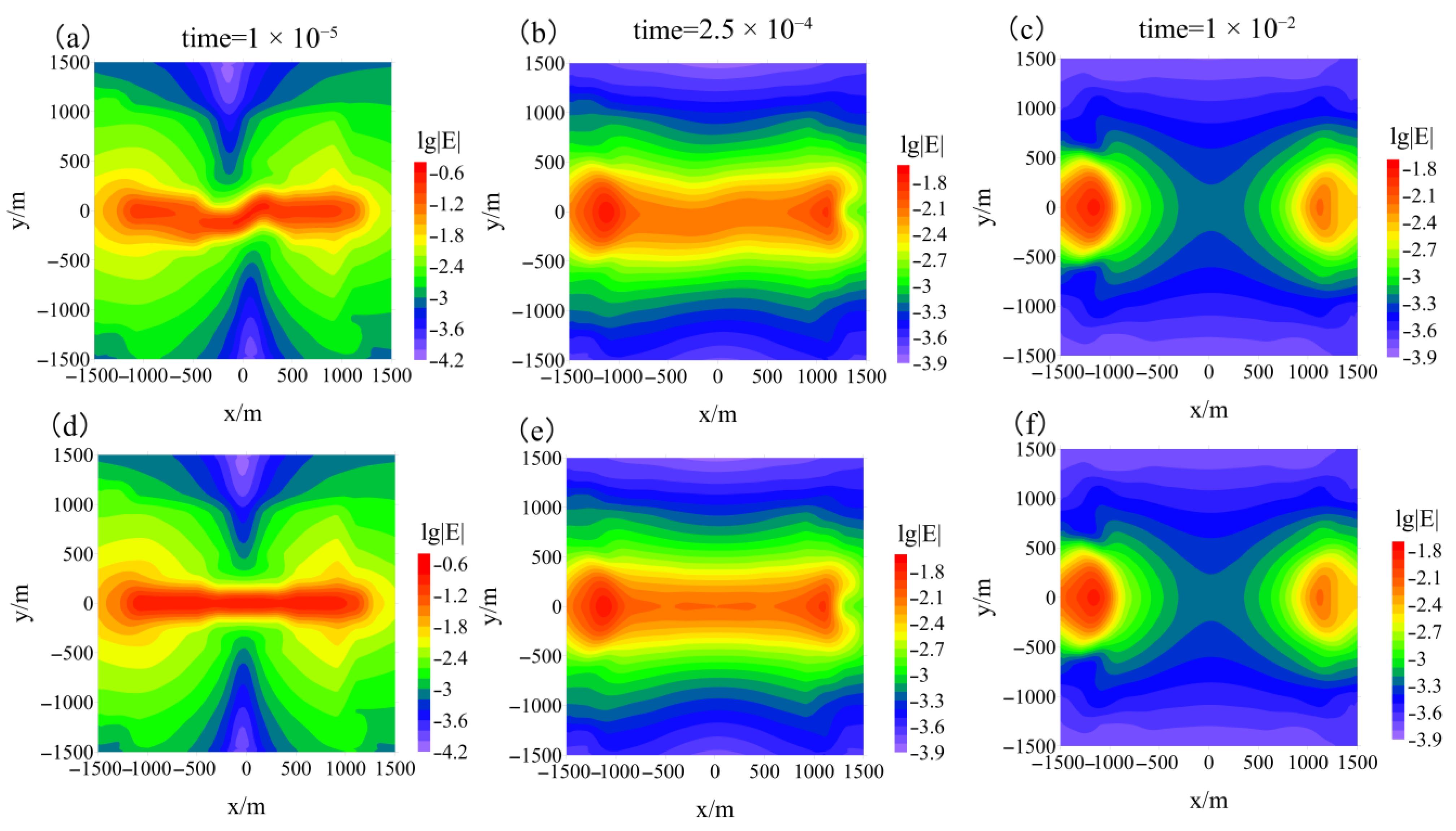
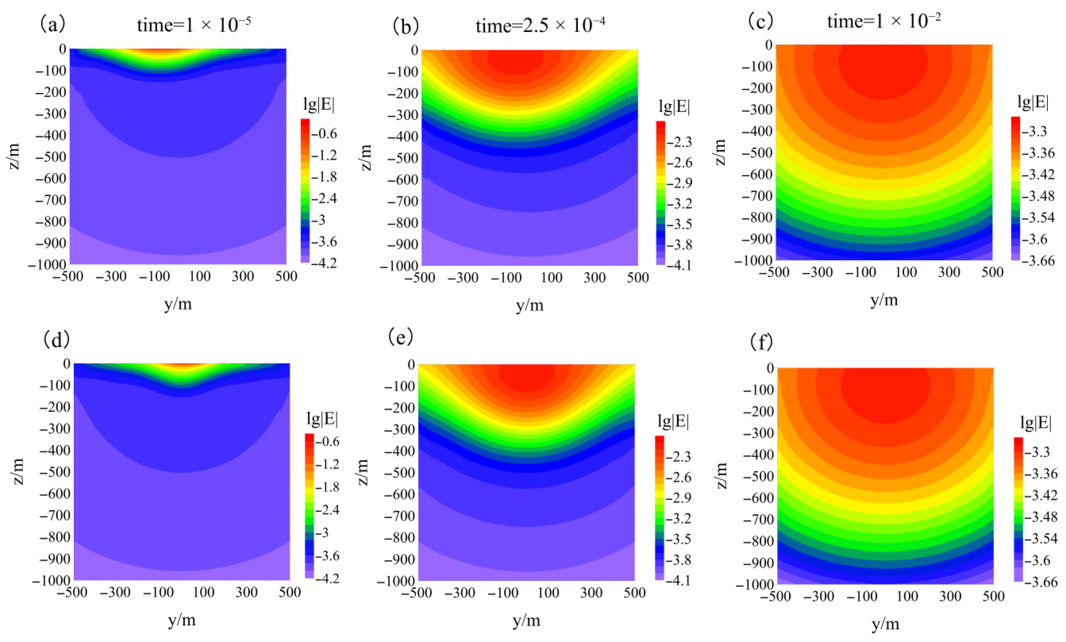
The SATEM method traditionally employs coils to measure the time derivative of the vertical magnetic field component $d{B}_z/dt$ [26,27]. Recent advancements in instrumentation have enabled direct measurements of the vertical magnetic field component $B_z$ [6]. In this study, we analyze the influence of the curved source geometry on both $d{B}_z/dt$ and $B_z$ measurements acquired in the airborne receiver.

Figure 5 illustrates the $B_z$ distribution in the oxy plane at various time instants for both linear and curved sources, where Figure 5a–c represent the curved source responses and Figure 5d–f depict the linear source responses. At an early time (t = 10⁻⁵ s), the maximum magnetic field intensity near the source follows the geometric configuration of the source, resulting in pronounced differences between the magnetic field distributions of curved and linear sources. As time progresses, the maximum magnetic field intensity gradually diffuses outward, diminishing the influence of the source geometry and progressively reducing the differences in magnetic field distribution near the source. At a late time (t = 0.01 s), the magnetic field distributions for curved and linear sources converge to near-identical patterns.

In practical applications, magnetic field responses are typically recorded within a specific survey area at a certain offset from the source, as indicated by the green wireframe in Figure 2, representing the receiving area with offsets ranging from 200 m to 1000 m. Figure 6 presents the $B_z$ distribution in the plane within this airborne receiving area at different time instants, with Figure 6a–c showing the curved source responses and Figure 6d–f displaying the linear source responses. Figure 6 clearly demonstrates that the source geometry significantly influences the magnetic field distribution in the proximal survey area. The magnetic field response of the linear source exhibits uniform distribution along the x-direction with a gradual attenuation along the y-direction. In contrast, the asymmetric configuration of the curved source produces non-uniform distributions along the x-direction, generating significant anomalies in the proximal survey area.

At t = 10⁻⁵ s, within the range x = −500 m to 0 m, the measurement profile at y = −200 m is positioned in close proximity to the curved source, manifesting as a region of maximum magnetic field intensity. Conversely, within the range x = 0 m to 500 m, the measurement profile at y = −200 m is situated farther from the curved source, and the maximum magnetic field has not yet propagated to this region. The magnetic field maximum diffuses progressively along the y-direction with time. At t = 2.5 × 10⁻⁴ s, within the range x = −500 m to 0 m, the maximum magnetic field has diffused to the region y = −400 m, while within the range x = 0 m to 500 m, the maximum magnetic field has just reached the vicinity of y = −200 m. At t = 0.01 s, as evident from comparing Figure 6c,f, the maximum magnetic field has diffused to the maximum offset at y = −1000 m, and the magnetic field within the receiving region exhibits a uniform distribution along the x-direction, with minimal influence from the source geometry.

Figure 7 illustrates the $d{B}_z/dt$ distribution in the oxy plane at various time instants for both linear and curved sources, where Figure 7a–c represent the curved source responses and Figure 7d–f depict the linear source responses. Figure 8 presents the $d{B}_z/dt$ distribution in the plane within the airborne receiving area at different time instants, with Figure 8a–c showing the curved source responses and Figure 8d–f displaying the linear source responses. The influence of the source geometry on $d{B}_z/dt$ distribution exhibits patterns analogous to those observed in the $B_z$ distribution. Both field components manifest as distinct anomalies in the proximal survey area during the early transient stage.

To further analyze these effects, we generated delay time profiles along survey lines at varying offsets. Delay time profiles are widely used to represent the transverse change characteristics of the responses [28]. Each line in the figure represents the observation data of different spatial positions at the same time, and the lines from top to bottom in the figure are correlated with the observation data from an early to a late time. Figure 9 presents the delay time profiles of $B_z$ responses for both linear and curved sources at different offset distances. Figure 9a–c correspond to curved source responses at offsets of 200 m, 500 m, and 800 m, respectively, while Figure 9d–f correspond to linear source responses at identical offsets. The delay time profiles for linear sources exhibit parallel contours across all offset distances, whereas the profiles for curved sources display complex patterns. At an offset of y = −200 m, the multichannel profile of the curved source exhibits pronounced depressions and elevations. A direct interpretation of these curved source profiles using linear source response models would generate erroneous high- and low-resistivity anomalies in the shallow subsurface. At an offset of y = −500 m, the multichannel profile of the curved source displays partial undulations and tilting; however, the profile distortion is less severe compared to that observed at y = −200 m. Interpretation using linear source models would still produce false low-resistivity anomalies and tilted structures in the shallow subsurface. At an offset of y = −800 m, the multichannel profile of the curved source becomes virtually indistinguishable from that of the linear source, indicating that the influence of source curvature becomes negligible at this distance.

Figure 10 presents the delay time profiles of $d{B}_z/dt$ responses for both linear and curved sources at different offset distances. Figure 10a–c correspond to curved source responses at offsets of 200 m, 500 m, and 800 m, respectively, while Figure 10d–f correspond to linear source responses at the same offsets. Similarly, the effect of the source geometry on the multichannel profiles of $d{B}_z/dt$ responses is consistent with the patterns observed in the $B_z$ response profiles, confirming that both field components are affected in a comparable manner by the source geometry.

3.2. 3D Model

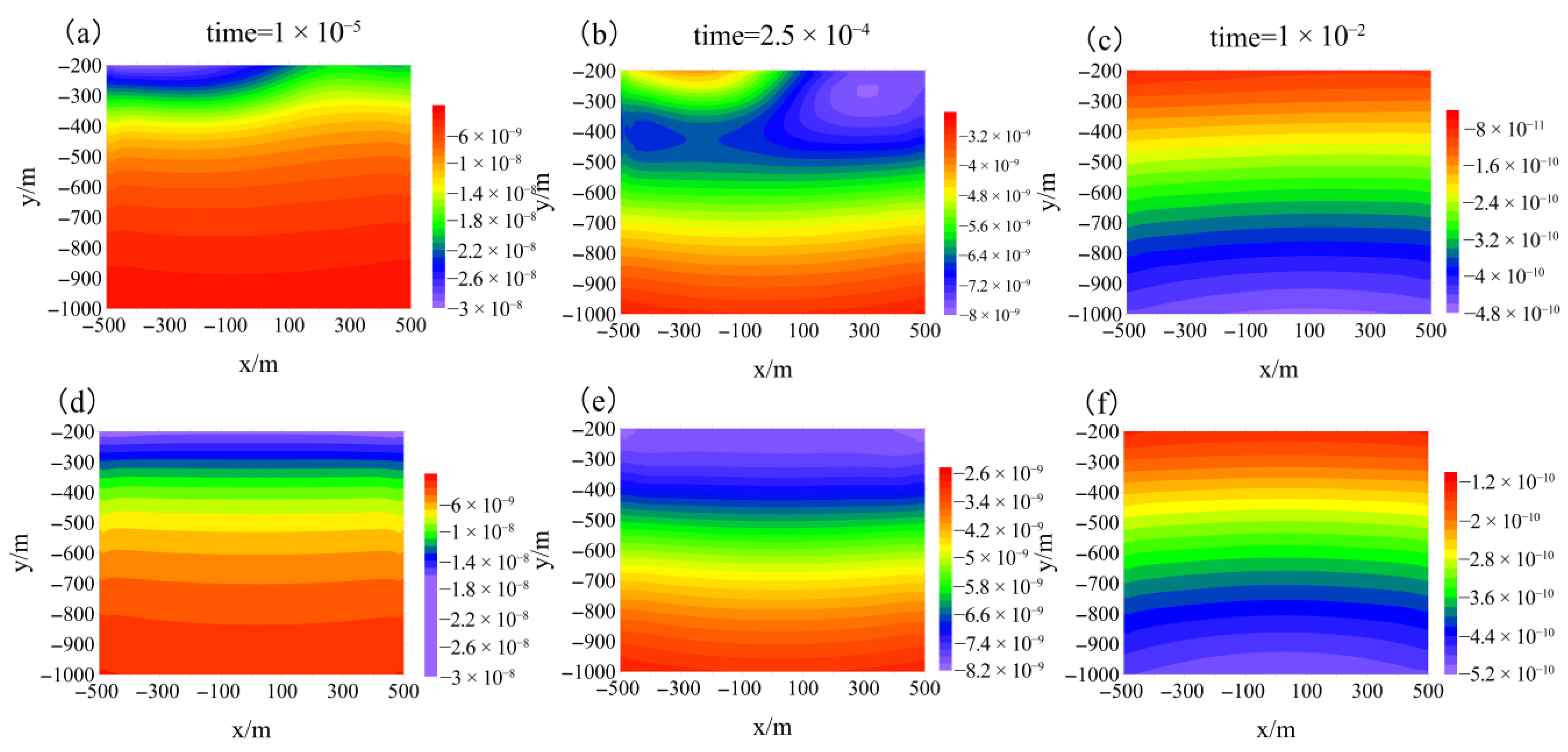
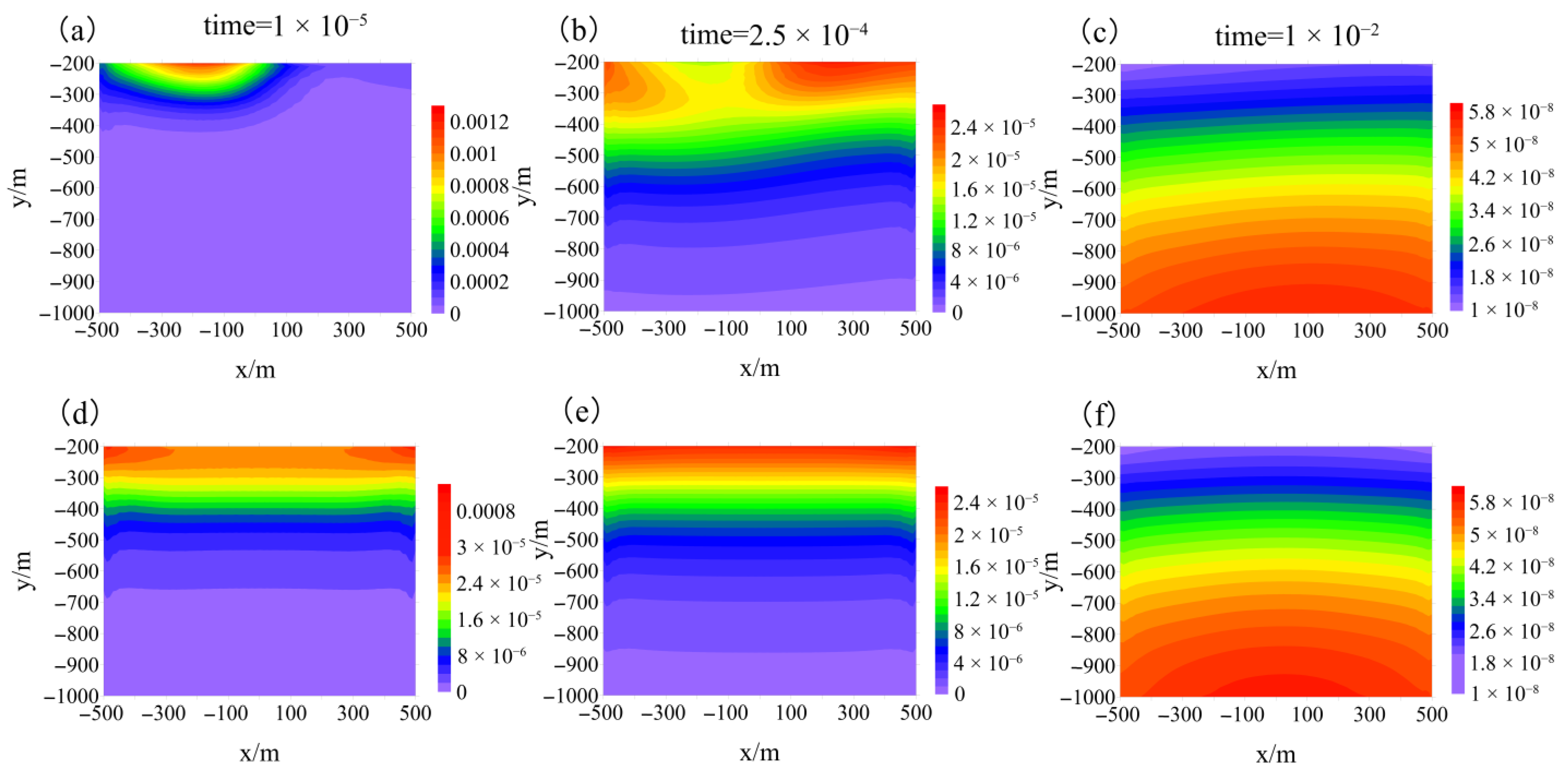
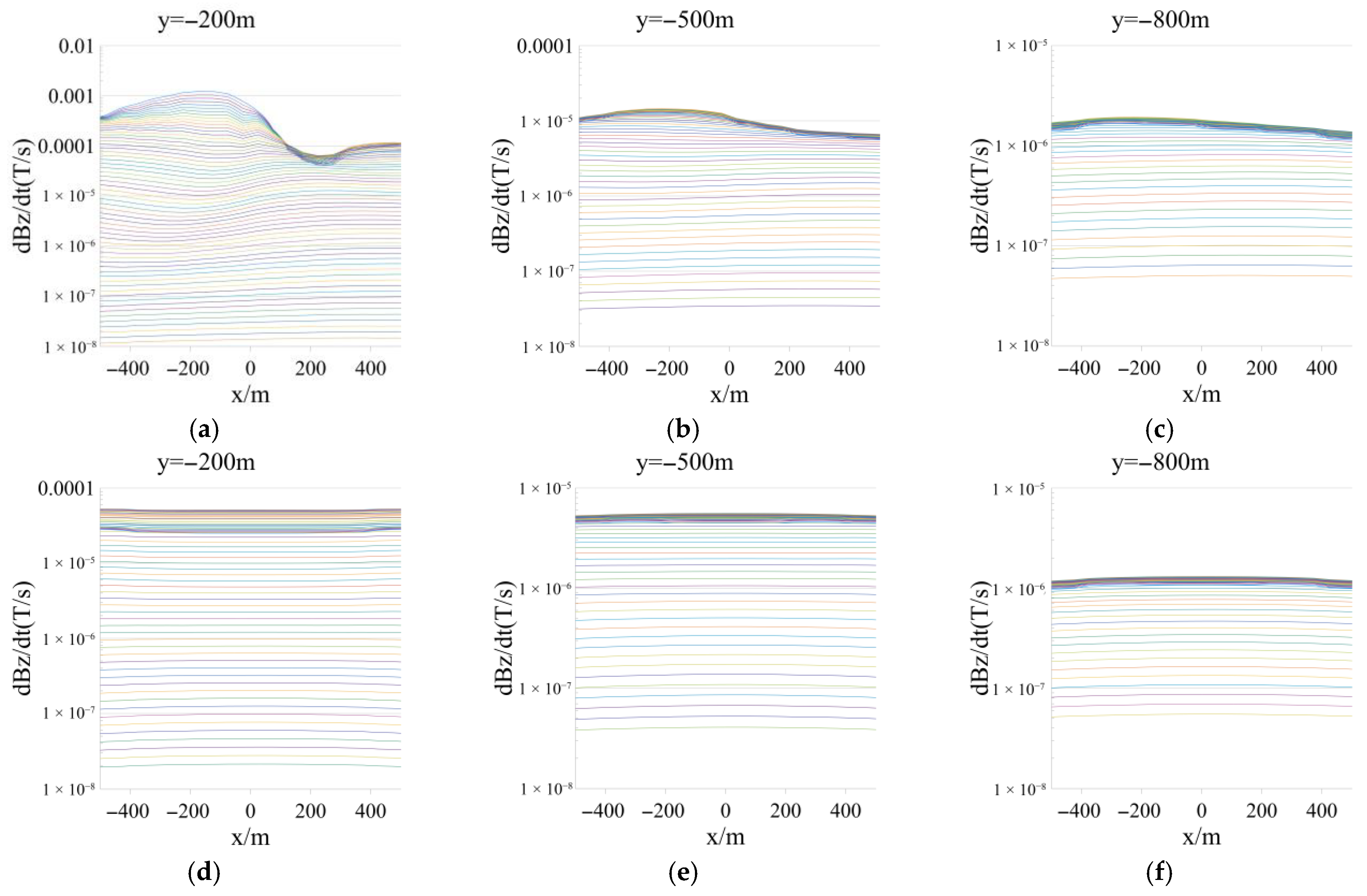
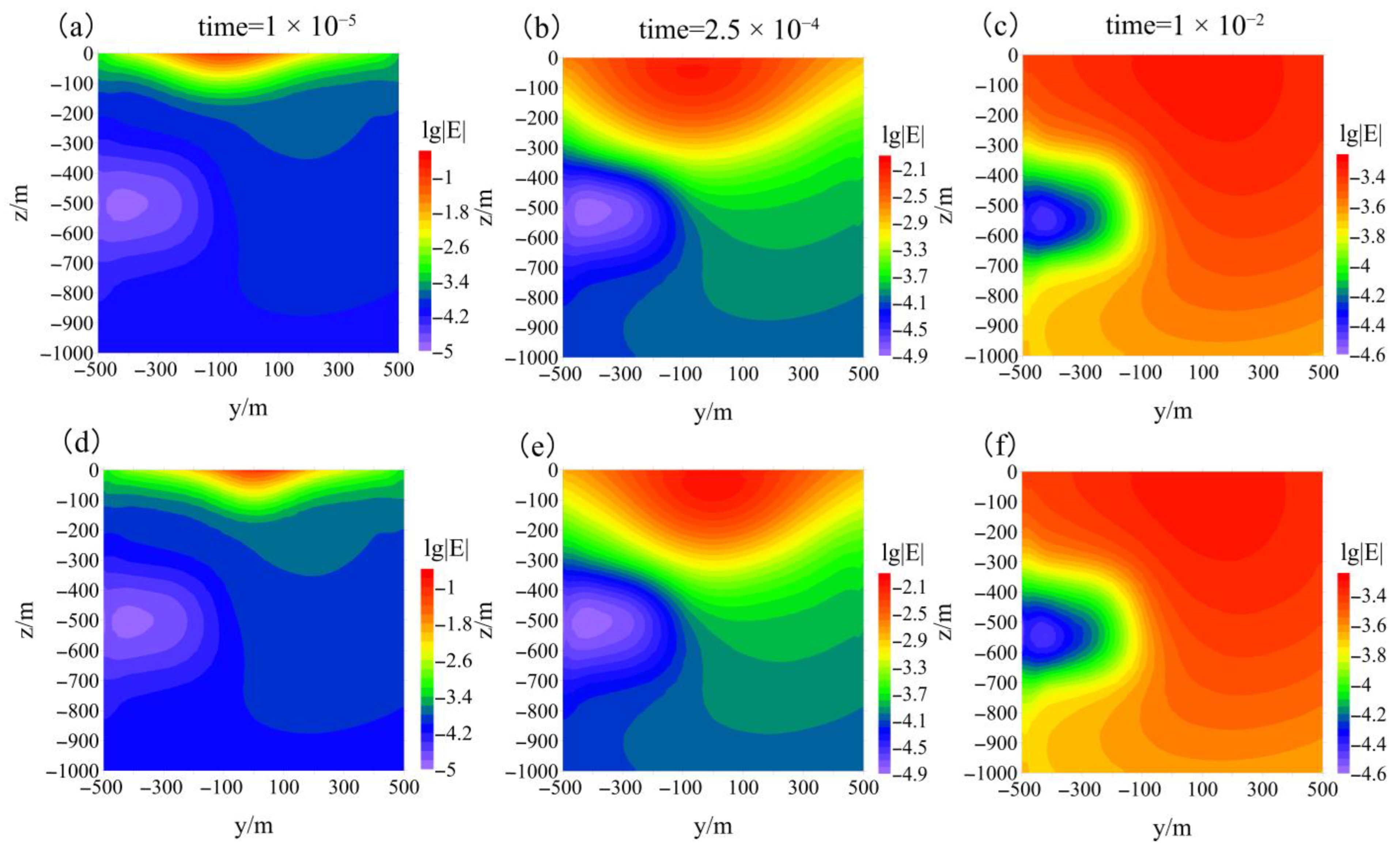
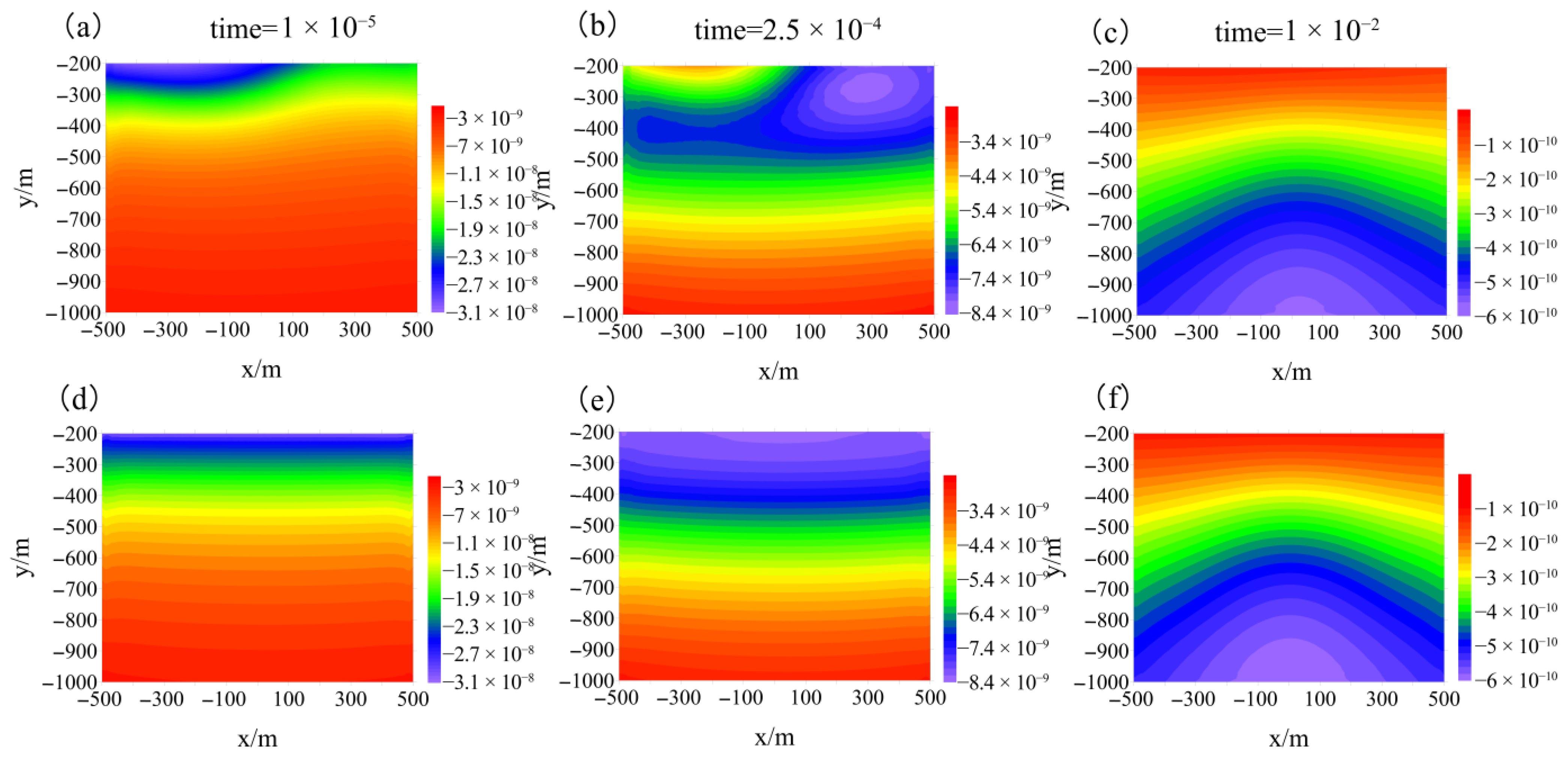
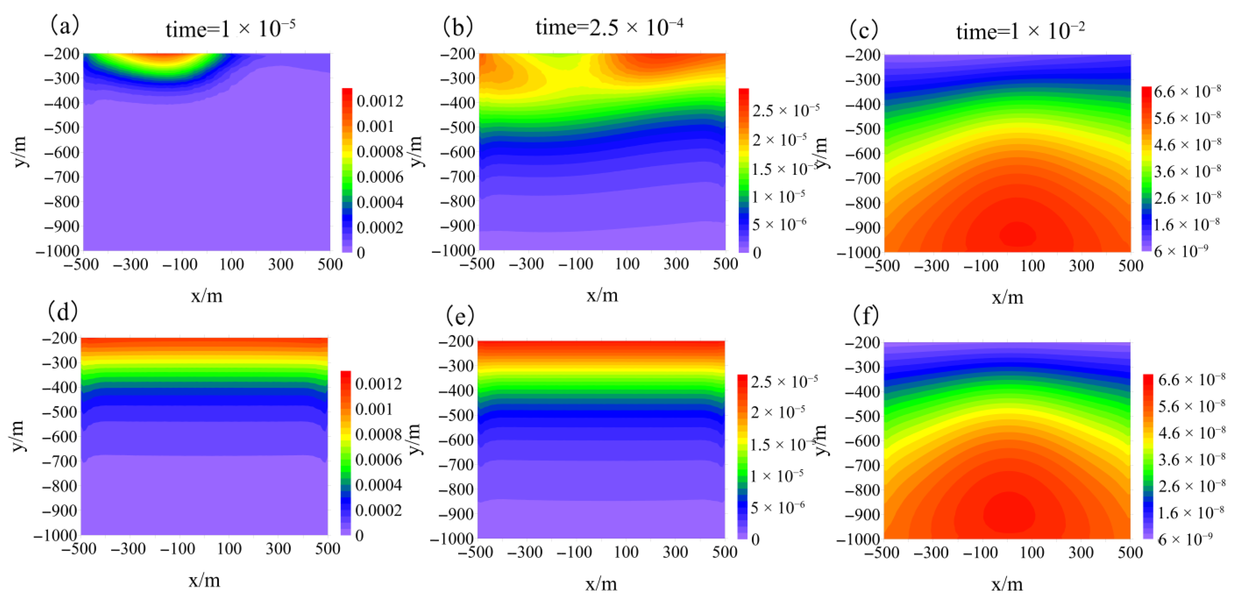
3.2.1. Electric Fields in the Earth

Figure 11 illustrates the electric field distribution in the surface oxy plane at various time instants for both linear and curved sources, where Figure 11a–c represent the curved source responses and Figure 11d–f depict the linear source responses. In the presence of the 3D low-resistivity anomaly, the electric field distribution undergoes significant distortion, with the current being preferentially channeled toward the conductive body. Consequently, a minimum in the electric field magnitude develops within the region occupied by the 3D anomaly, consistent with the findings reported by Gunderson et al. [15]. A comparative analysis of Figure 4 and Figure 11 reveals that the shallow electric field distribution in the 3D model closely resembles that of the homogeneous half-space model, except for the localized low-amplitude distortion coinciding with the 3D anomaly. This observation indicates that the source geometry predominantly influences the shallow electric field distribution during early time periods while having minimal impact on the deep electric field distribution at later times. Conversely, the 3D conductive anomaly primarily affects the electric field distribution at depth. These results suggest that the influences of the source geometry and the 3D conductive anomaly on the electric field distribution can be considered effectively independent of each other.

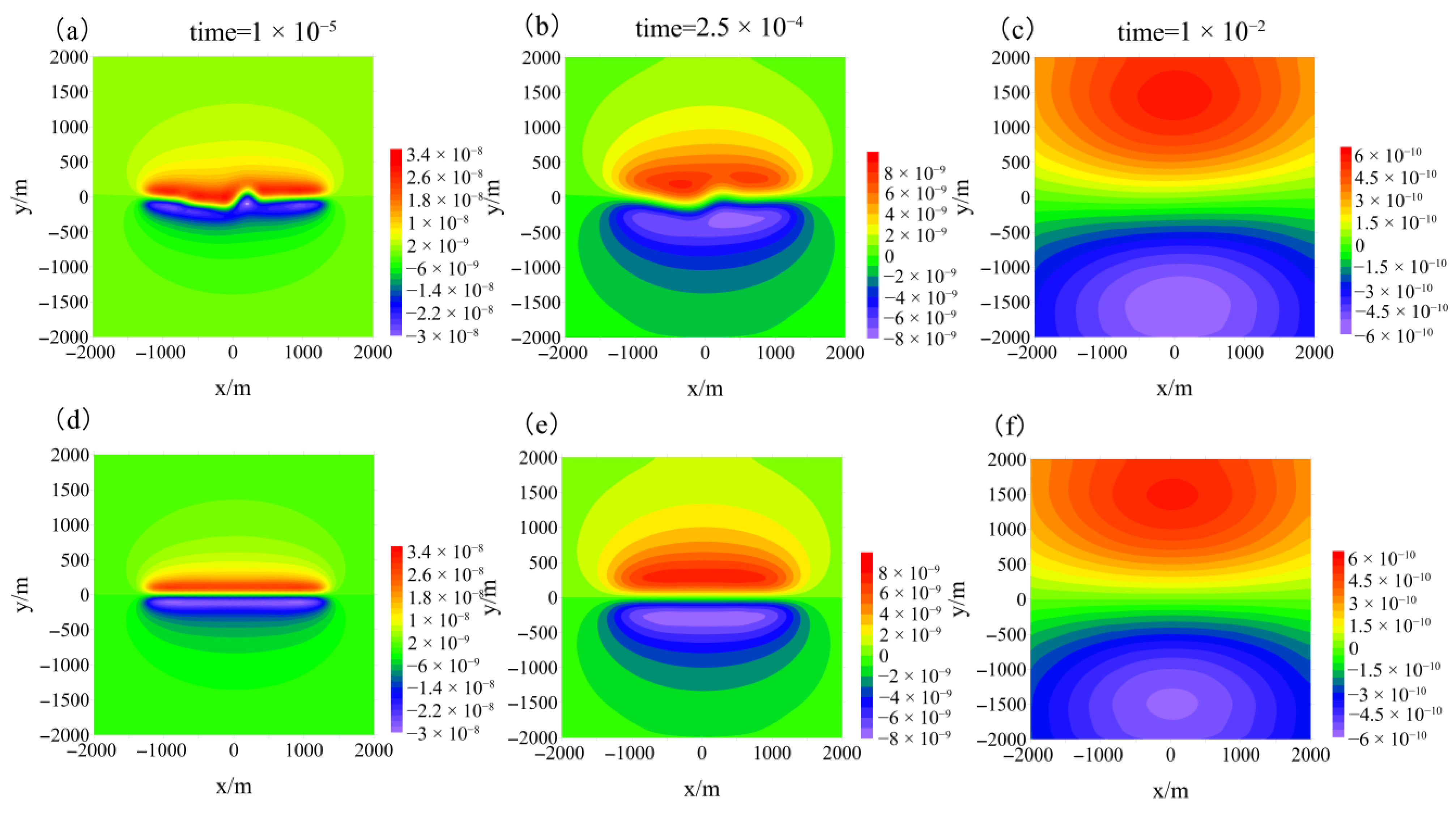
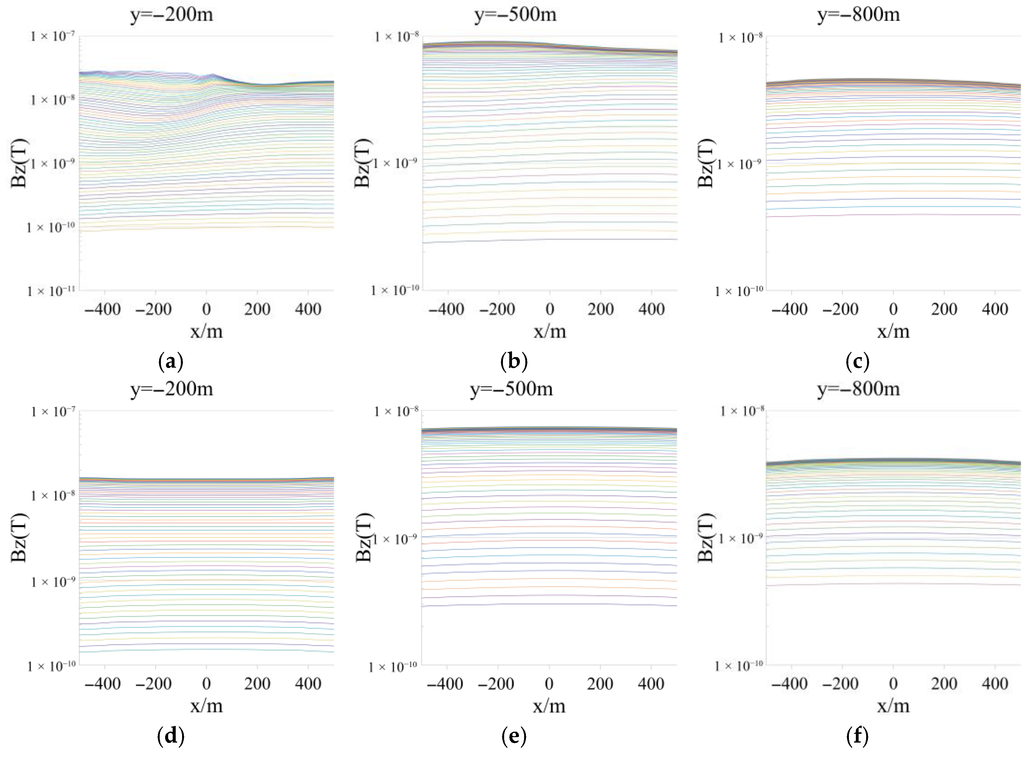
3.2.2. Magnetic Fields in the Air

Figure 12 illustrates the $B_z$ distribution in the plane within the airborne receiving area at various time instants, where Figure 12a–c represent the curved source responses, and Figure 12d–f depict the linear source responses. A comparative analysis of Figure 5 and Figure 12 reveals that the 3D conductive body predominantly influences the $B_z$ response at 0.01 s. The distributions shown in Figure 12c,f exhibit remarkable similarity, both clearly displaying anomalies attributable to the 3D conductive structure, while a subtle oblique distribution of the magnetic field is observed in the proximal region. The magnetic field distributions at 10⁻⁵ s and 2.5 × 10⁻⁴ s closely resemble those of the homogeneous half-space model, with the influence of the source geometry being distinctly visible in regions of small offset, whereas the impact of the 3D conductive structure on the magnetic field remains negligible at these earlier times.

Figure 13 presents the $d{B}_z/dt$ distribution in the plane within the airborne receiving area at various time instants, where Figure 13a–c represent the curved source responses, and Figure 13d–f depict the linear source responses. In comparison with $B_z$, the $d{B}_z/dt$ component exhibits analogous characteristics: the source geometry predominantly affects $d{B}_z/dt$ at small offsets, while the 3D conductive structure influences $d{B}_z/dt$ at large offsets at the later time of 0.01 s.

To further elucidate these relationships, we present the delay time profiles of the magnetic field responses along different offset lines. Figure 14 displays the delay time profiles of $B_z$ responses at various offsets. Figure 14a–c correspond to the curved source responses at 200 m, 500 m, and 800 m, respectively, while Figure 14d–f correspond to the linear source responses at the same respective offsets. Similarly, Figure 15 presents the delay time profiles of $d{B}_z/dt$ responses at various offsets. Figure 15a–c correspond to curved source responses at 200 m, 500 m, and 800 m, respectively, while Figure 15d–f correspond to linear source responses at the same respective offsets. These multichannel profiles illustrate the temporal evolution of the magnetic field from early times (10⁻⁵ s) to late times (0.01 s). A comparative analysis of Figure 14 and Figure 15 with Figure 9 and Figure 10 clearly demonstrates that the source geometry primarily induces distortion in the early-time magnetic field responses along the measurement profile, whereas the 3D conductive structure predominantly causes an enhancement of the late-time magnetic field responses along the same profile.

4. Discussion

We employed synthetic modeling to analyze how the source geometry influences the SATEM response. A typical curved source configuration was designed to calculate the SATEM electric and magnetic field responses, and its influence on SATEM measurements was systematically evaluated through comparison with the theoretical linear source model response. Initially, we calculated the SATEM electric and magnetic field responses for homogeneous half-space models with both linear and curved sources. The electric and magnetic field distributions of the linear source exhibit straightforward patterns, facilitating a clear comparative analysis of the curved source’s influence on SATEM’s electromagnetic response. The results demonstrate that upon current termination in the transmitter, the induced currents concentrate predominantly near conductive regions, with electric and magnetic fields displaying spatial distributions that reflect the source geometry. As time progresses, the current diffuses downward, and the influence of the source geometry diminishes. Consequently, the source geometry primarily affects early-time electromagnetic responses in proximity to the source while exerting minimal influence on late-time responses at large offsets. Subsequently, we calculated the SATEM electric and magnetic field responses for a 3D model containing a low-resistivity anomaly. Comparative analysis reveals that 3D conductive anomalies at certain burial depths predominantly affect late-time responses. Notably, the influences of the source geometry and 3D conductive structures on electromagnetic field distributions operate independently of each other.

Based on fieldwork design, this paper proposes a curved source that bends along the horizontal plane and investigates its impact on SATEM responses. During actual field exploration, the shape of the transmitting source is constrained by terrain and road conditions, resulting in various curved configurations. Different source shapes produce varying effects on SATEM responses. The source may exhibit significant curvature [29], leading to more pronounced impacts on SATEM responses. Furthermore, terrain undulations can cause the transmitting source to bend in 3D space, creating more complex influences on SATEM responses. Future systematic studies on how different types of transmitting sources affect SATEM responses will enhance our understanding of observational data collected under diverse field terrain conditions.

Due to instrumentation limitations, this study only addresses the impact of the source geometry on the vertical component of the magnetic field. Gunderson et al. [15], through an analysis of ground-based three-component magnetic field response characteristics, concluded that horizontal magnetic field components are more advantageous for 3D target localization. Nazari et al. [21] also discussed improvements in the inversion results through three-component observations. In the future, as three-component magnetic field observation equipment becomes more widely available, the influence of the source geometry on horizontal magnetic field components warrants further investigation.

Geophysical methods require an inversion interpretation of observational data [7,8,9,29,30,31,32]. The shape of the transmitting source significantly impacts observational data, particularly causing severe distortion in early-time data within small offset regions. Since electromagnetic field information attenuates with offset distance and observation time, the data amplitude is larger in early-time small offset regions and smaller in late-time large offset regions. If the influence of the source shape is disregarded and an ideal linear source is directly employed for optimization-based inversion of all data, shallow false anomalies will inevitably appear in small offset regions, while deep true anomalies in large offset regions will be suppressed. Therefore, information about the source shape and spatial distribution must be incorporated into the inversion process [29].

5. Conclusions

Our experiments demonstrate that the transmitting source shape significantly affects observational data. Since our theoretical model is simpler than actual geological models, and field transmitting sources have diverse spatial distributions, the impact of the source spatial distribution on observational data is even more complex in practice. As the source shape primarily causes distortion in early-time response data in small offset regions, to ensure effective SATEM detection, we recommend primarily using late-time data from large offset regions. However, late-time data from large offset regions has a very small signal amplitude and is highly susceptible to background noise interference. Early-time response data from small offset regions has a larger signal amplitude and is less affected by background noise. Therefore, considering these factors comprehensively, when conducting SATEM work in the field, the shape of the transmitting source should be recorded in detail to ensure that early-time data from small offset regions remains usable, thereby enabling the effective detection of three-dimensional subsurface electrical structures across a wide range—from small to large offset regions and from shallow to deep earth.

References

1. Wu, X.; Rao, L.-T.; Luan, X.-D.; Shi, J.-J.; Wang, Y.-B. Design and Development of a Semiairborne Transient Electromagnetic System. Geophysics 2024, 89, E255–E266. [Google Scholar] [CrossRef]
2. Zhou, N.; Zhang, S. Comparison of Semi-Airborne Transient Electromagnetic Data from Double-Line and Single-Line Grounded-Wire Sources. J. Appl. Geophys. 2022, 197, 104538. [Google Scholar] [CrossRef]
3. Becken, M.; Kotowski, P.O.; Schmalzl, J.; Symons, G.; Brauch, K. Semi-Airborne Electromagnetic Exploration Using a Scalar Magnetometer Suspended below a Multicopter. First Break 2022, 40, 37–46. [Google Scholar] [CrossRef]
4. Ma, Z.; Di, Q.; Lei, D.; Gao, Y.; Zhu, J.; Xue, G. The Optimal Survey Area of the Semi-Airborne TEM Method. J. Appl. Geophys. 2020, 172, 103884. [Google Scholar] [CrossRef]
5. Chen, C.; Sun, H. Characteristic Analysis and Optimal Survey Area Definition for Semi-Airborne Transient Electromagnetics. J. Appl. Geophys. 2020, 180, 104134. [Google Scholar] [CrossRef]
6. Steuer, A.; Smirnova, M.; Becken, M.; Schiffler, M.; Günther, T.; Rochlitz, R.; Yogeshwar, P.; Mörbe, W.; Siemon, B.; Costabel, S.; et al. Comparison of Novel Semi-Airborne Electromagnetic Data with Multi-Scale Geophysical, Petrophysical and Geological Data from Schleiz, Germany. J. Appl. Geophys. 2020, 182, 104172. [Google Scholar] [CrossRef]
7. Kotowski, P.O.; Becken, M.; Rochlitz, R.; Schmalzl, J.; Ueding, S.; Tolksdorf, P.; Wilhelm, A.; Symons, G. Semi-Airborne Electromagnetic Exploration of Deep Sulfide Deposits with UAV-Towed Magnetometers—Part 1: Processing Modeling. Geophysics 2025, 90, 1–52. [Google Scholar] [CrossRef]
8. Rochlitz, R.; Günther, T.; Kotowski, P.O.; Becken, M. Semi-Airborne Electromagnetic Exploration of Deep Sulfide Deposits with UAV-Towed Magnetometers—Part 2: Inversion Resolution Analysis. Geophysics 2025, 90, 1–63. [Google Scholar] [CrossRef]
9. Mörbe, W.; Yogeshwar, P.; Tezkan, B.; Kotowski, P.; Thiede, A.; Steuer, A.; Rochlitz, R.; Günther, T.; Brauch, K.; Becken, M. Large-Scale 3D Inversion of Semi-Airborne Electromagnetic Data—Topography and Induced Polarization Effects in a Graphite Exploration Scenario. Geophysics 2024, 89, B339–B352. [Google Scholar] [CrossRef]
10. Smirnova, M.; Juhojuntti, N.; Becken, M.; Smirnov, M. Exploring Kiruna Iron Ore Fields with Large-Scale, Semi-Airborne, Controlled-Source Electromagnetics. First Break 2020, 38, 35–40. [Google Scholar] [CrossRef]
11. Davidenko, Y.; Hallbauer-Zadorozhnaya, V.; Bashkeev, A.; Parshin, A. Semi-Airborne UAV-TEM System Data Inversion with S-Plane Method—Case Study over Lake Baikal. Remote Sens. 2023, 15, 5310. [Google Scholar] [CrossRef]
12. Lu, K.; Li, X.; Fan, Y.; Zhou, J.; Qi, Z.; Li, W.; Li, H. The Application of Multi-Grounded Source Transient Electromagnetic Method in the Detections of Coal Seam Goafs in Gansu Province, China. J. Geophys. Eng. 2021, 18, 515–528. [Google Scholar] [CrossRef]
13. Cheng, W.; Sun, N.; Qi, Z.; Cao, H.; Li, X. The Application of GATEM in Tunnel Geologic Risk Survey Based on Complex Terrain. Geophysics 2024, 89, B453–B465. [Google Scholar] [CrossRef]
14. Smith, R.S.; Annan, A.P.; McGowan, P.D. A Comparison of Data from Airborne, Semi-airborne, and Ground Electromagnetic Systems. Geophysics 2001, 66, 1379–1385. [Google Scholar] [CrossRef]
15. Gunderson, B.M.; Newman, G.A.; Hohmann, G.W. Three-dimensional Transient Electromagnetic Responses for a Grounded Source. Geophysics 1986, 51, 2117–2130. [Google Scholar] [CrossRef]
16. Streich, R.; Becken, M. Electromagnetic Fields Generated by Finite-Length Wire Sources: Comparison with Point Dipole Solutions: EM Fields Generated by Finite-Length Wire Sources. Geophys. Prospect. 2011, 59, 361–374. [Google Scholar] [CrossRef]
17. Chen, W.-Y.; Xue, G.-Q.; Cui, J.-W. Analysis on the influence from the shape of electric source TEM transmitter. Prog. Geophys. 2015, 30, 126–132. [Google Scholar] [CrossRef]
18. Li, Z.-H.; Huang, Q.-H. 1D forward modeling and inversion algorithm for grounded galvanic source TEM sounding with an arbitrary horizontal wire. Prog. Geophys. 2018, 33, 1515–1525. [Google Scholar] [CrossRef]
19. Zhou, N.; Xue, G.; Hou, D.; Lu, Y. An Investigation of the Effect of Source Geometry on Grounded-Wire TEM Surveying with Horizontal Electric Field. J. Environ. Eng. Geophys. 2018, 23, 143–151. [Google Scholar] [CrossRef]
20. Zhou, Z.; Weng, A.; Wang, X.; Zou, Z.; Tang, Y.; Wang, T. Source Shape Impact on Controlled Source EM Surveys. J. Appl. Geophys. 2019, 171, 103858. [Google Scholar] [CrossRef]
21. Nazari, S.; Rochlitz, R.; Günther, T. Optimizing Semi-Airborne Electromagnetic Survey Design for Mineral Exploration. Minerals 2023, 13, 796. [Google Scholar] [CrossRef]
22. Liu, W.; Farquharson, C.G.; Zhou, J.; Li, X. A Rational Krylov Subspace Method for 3D Modeling of Grounded Electrical Source Airborne Time-Domain Electromagnetic Data. J. Geophys. Eng. 2019, 16, 451–462. [Google Scholar] [CrossRef]
23. Haber, E. Computational Methods in Geophysical Electromagnetics; Society for Industrial and Applied Mathematics: Philadelphia, PA, USA, 2014; ISBN 978-1-61197-379-2. [Google Scholar]
24. Zhou, J.; Liu, W.; Li, X.; Qi, Z. 3D Transient Electromagnetic Modeling Using a Shift-and-Invert Krylov Subspace Method. J. Geophys. Eng. 2018, 15, 1341–1349. [Google Scholar] [CrossRef]
25. Zhang, Y.-Y.; Li, X.; Yao, W.-H.; Zhi, Q.-Q.; Li, J. Multi-component full field apparent resistivity definition of multi-source ground-airborne transient electromagnetic method with galvanic sources. Chin. J. Geophys. 2015, 58, 2745–2758. (In Chinese) [Google Scholar] [CrossRef]
26. Mogi, T.; Tanaka, Y.; Kusunoki, K.; Morikawa, T.; Jomori, N. Development of Grounded Electrical Source Airborne Transient EM (GREATEM). Explor. Geophys. 1998, 29, 61–64. [Google Scholar] [CrossRef]
27. Mogi, T.; Kusunoki, K.; Kaieda, H.; Ito, H.; Jomori, A.; Jomori, N.; Yuuki, Y. Grounded Electrical-Source Airborne Transient Electromagnetic (GREATEM) Survey of Mount Bandai, North-Eastern Japan. Explor. Geophys. 2009, 40, 1–7. [Google Scholar] [CrossRef]
28. Nabighian, M.N.; Macnae, J.C. Time Domain Electromagnetic Prospecting Methods. In Electromagnetic Methods in Applied Geophysics: Volume 2, Application, Parts A and B; Investigations in Geophysics; Society of Exploration Geophysicists: Houston, TX, USA, 1991; pp. 427–520. ISBN 978-1-56080-022-4. [Google Scholar]
29. Mörbe, W.; Rochlitz, R.; Kotowski, P.; Tezkan, B.; Yogeshwar, P. Multi-Source 3D Imaging of a Graphite Deposit Combining Drone-Based Semi-Airborne and Ground-Based Electromagnetics. In Proceedings of the 26th EM Induction Workshop, Beppu, Japan, 7–13 September 2024. [Google Scholar]
30. He, Y.; Xue, G.; Chen, W.; Tian, Z. Three-Dimensional Inversion of Semi-Airborne Transient Electromagnetic Data Based on a Particle Swarm Optimization-Gradient Descent Algorithm. Appl. Sci. 2022, 12, 3042. [Google Scholar] [CrossRef]
31. Yang, H.; Cai, H.; Liu, M.; Xiong, Y.; Long, Z.; Li, J.; Hu, X. Three-Dimensional Inversion of Semi-Airborne Transient Electromagnetic Data Based on Finite Element Method. Near Surf. Geophys. 2022, 20, 661–678. [Google Scholar] [CrossRef]
32. Rochlitz, R.; Becken, M.; Günther, T. Three-Dimensional Inversion of Semi-Airborne Electromagnetic Data with a Second-Order Finite-Element Forward Solver. Geophys. J. Int. 2023, 234, 528–545. [Google Scholar] [CrossRef]
Figure 1. Schematic representation of the electric dipole coordinate system positioned on a horizontally stratified earth surface.
Applsci 15 04389 g001
Figure 2. Schematic representation of the 3D model and SATEM transmitter and receiver distribution.
Applsci 15 04389 g002
Figure 3. Electric field (V/m) in oxy plane for the half-space model at different time instants. Panels (ac) represent the curved source response, while panels (df) illustrate the linear source response.
Applsci 15 04389 g003
Figure 4. Electric field (V/m) in oyz plane for the half-space model at different time instants. Panels (ac) represent the curved source response, while panels (df) illustrate the linear source response.
Applsci 15 04389 g004
Figure 5. B z (A/m) of oxy plane in the air for the half-space model at different time instants. Panels (ac) represent the curved source response, while panels (df) illustrate the linear source response.
Applsci 15 04389 g005
Figure 6. B z (A/m) in the plane within this airborne receiving area for the half-space model at different time instants. Panels (ac) represent the curved source response, while panels (df) illustrate the linear source response.
Applsci 15 04389 g006
Figure 7. d B z / d t (V/m2) of oxy plane in the air for the half-space model at different time instants. Panels (ac) represent the curved source response, while panels (df) illustrate the linear source response.
Applsci 15 04389 g007
Figure 8. d B z / d t (V/m2) in the plane within this airborne receiving area for the half-space model at different time instants. Panels (ac) represent the curved source response, while panels (df) illustrate the linear source response.
Applsci 15 04389 g008
Figure 9. Delay time profile of B z (A/m) at different offsets for half-space model. Panels (ac) represent curved source response, and panels (df) illustrate linear source response.
Applsci 15 04389 g009
Figure 10. Delay time profile of d B z / d t (V/m2) at different offsets for half-space model. Panels (ac) represent curved source response, and panels (df) are for linear source response.
Applsci 15 04389 g010
Figure 11. Electric field (V/m) in oyz plane for the 3D model at different time instants. Panels (ac) represent the curved source response, while panels (df) illustrate the linear source response.
Applsci 15 04389 g011
Figure 12. B z (A/m) in the plane within this airborne receiving area for the 3D model at different time instants. Panels (ac) represent the curved source response, while panels (df) illustrate the linear source response.
Applsci 15 04389 g012
Figure 13. d B z / d t (V/m2) in the plane within this airborne receiving area for the 3D model at different time instants. Panels (ac) represent the curved source response, while panels (df) illustrate the linear source response.
Applsci 15 04389 g013
Figure 14. Delay time profile of B z (A/m) at different offsets for 3D model. Panels (ac) represent curved source response, and panels (df) illustrate linear source response.
Applsci 15 04389 g014
Figure 15. Delay time profile of d B z / d t (V/m2) at different offsets for 3D model. Panels (ac) represent curved source response, and panels (df) are for linear source response.
Applsci 15 04389 g015
Disclaimer/Publisher’s Note: The statements, opinions and data contained in all publications are solely those of the individual author(s) and contributor(s) and not of MDPI and/or the editor(s). MDPI and/or the editor(s) disclaim responsibility for any injury to people or property resulting from any ideas, methods, instructions or products referred to in the content.