

Data-Driven Approaches for Predicting and Forecasting Air Quality in Urban Areas


Abstract
1. Introduction
1.1. AI Used in Air Quality Measurement
1.2. IoT Employed in Air Quality Measurement
1.3. Paper Contributions
- Implementation and integration of six customized ML algorithms, six pre-implemented ML models using ML.NET, and seven customized DL algorithms designed to address the specific characteristics of AQ data;
- Comparative analysis of ML versus DL methodologies, including the identification of the best approach based on performance metrics using an innovative parameter proposed by the authors;
- Integration of a second model for window timeframe forecasting integrated into a user-friendly application, including a prediction model and a forecasting model;
- Proposing a decision-making framework based on the implemented models, using the Azure Communication Service for data-driven actions in AQ management.
2. Materials and Methods
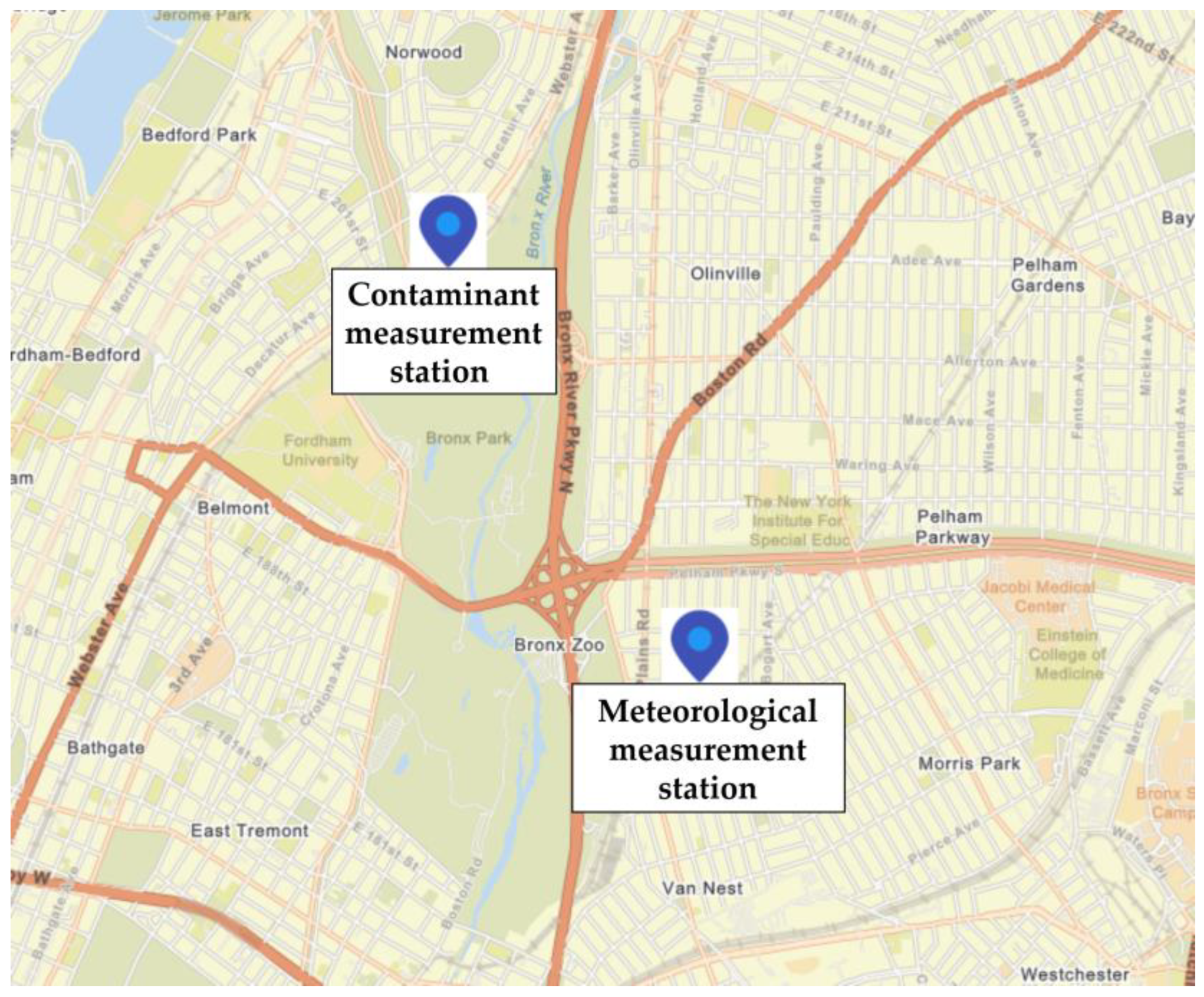
2.1. Data Import Process Description
- The table AirQualityDataBronx is populated with values corresponding to the data from 1 January 2020 to 31 December 2023, and NULL values will be used for each column;
- For each analyzed parameter, an API request to the EPA is made:
- ○
- Using the CsvHelper library, the C# script first reads the CSV file containing the AQ value for the first parameter analyzed;
- ○
- Each record from the CSV is parsed and transformed into an AirQualityRecord object, capturing the values for attributes such as the date, parameter type, and the corresponding AQI value for the parameter;
- ○
- The script establishes a connection to the SQL database;
- ○
- An SQL UPDATE command is run to modify the existing records in the AirQualityData table based on the new date;
- ○
- The global AQI is computed as the maximum value for the AQ_CO, AQ_NO2, AQ_SO2, AQ_PM2.5;
- A second API Request to Open NY is made to obtain a traffic dataset in the Bronx, representing the total number of cars transiting the county. To calculate the unit traffic data, the hourly traffic volume for each monitoring station in the Bronx was analyzed. At the source [63], the available dataset provided information on the number of vehicles passing through each station (broken down by inbound and outbound directions) at each hour of the day. The monitored locations are not explicitly mentioned, but the number of vehicles provided the information to compute the daily traffic volume for each station. The data are imported into the DailyTrafficData table.
- A third Request to the OMAP is made to retrieve the temperature, humidity, and wind speed values for each day in the 2020–2023 interval. The data are imported into the BronxWeatherDataHistory table;
- The data from the tables AirQualityDataBronx, DailyTrafficData, and BronxWeatherDataHistory are imported into a single table named BronxStats;
- The records for which one of the monitored parameters had a NULL value were at random, and we removed them due to missing data in the CSV files for several days, ensuring data integrity for analysis.
2.2. ML Custom-Made Versus Pre-Implemented Algorithms for AQI
- Random Forest Regression (RFR) uses decision tree decomposition in the training process, and next, it uses the mean prediction for each tree [72]. In the evaluated RFR, the hyperparameters/parameters were set as follows: the number of estimators (n_estimators) to 500, the maximum features in each tree (max_features) to 10, random state (random_state) to 0 and, the decision tree maximum depth (max_depth) was set to 15;
- Decision Tree Regression (DTR) is used for regression tasks, where the data are split into subsets based on feature values, creating a tree-like model of decisions. This approach allows for the modeling of complex relationships without requiring linear assumptions. Decision trees are valued for their interpretability and ability to handle numerical and categorical data. They can also manage missing values, making them versatile in practical applications [73,74]. In this case, the hyperparameters/parameters were set as follows: the decision tree maximum depth (max_depth) was set to 5 (sufficient depth to ensure an accurate prediction, with low execution time), the random state (random_state) to 42, the minimum number of samples per split (min_sample_split) was 4, the minimum number of samples per leaf (min_samples_leaf) was set to 2, and the criterion hyperparameter was set to “squared_error”, and the tree was split using minimum mean squared error (MSE);
- Linear Regression (LR) represents one of the simplest forms of regression analysis. This method assumes a straight-line relationship and is widely used due to its simplicity and ease of interpretation. The algorithm does not perform well in some situations when complex patterns are not identified, which leads to underfitting [75]. In this case, the algorithm calculates the parameter intercept (intercept_) or bias (whose value is 7.014022494795359), the coefficients (coef_) or weights for each of the eight features (respectively [−5.140072451758598, 0.3317304406559781, 3.1989070961349095, −0.1828119410953855, −0.03925884240140581, 0.00782994619292085, 0.00233905 795529826, 1.0876253401024537 × 10⁻⁶]), and a single CPU was used to evaluate the model;
- The K-nearest neighbors (KNN) algorithm estimates the target variable’s value by averaging the k-nearest neighbors in the feature space. This technique helps capture local patterns in the data and can adapt to various data distributions. Nonetheless, it tends to be computationally demanding, particularly with extensive datasets, since it necessitates calculating distances to every training sample [76]. We set the hyperparameters/parameters as follows: the algorithm uses 5 neighbors (n_neighbors), with all neighbors weighted equally (weights = “uniform”), 2 power parameters (p = 2) for the Minkowski metric, and a single CPU;
- Support Vector Regression (SVR) is a regression algorithm employed to approximate the output, knowing the input [77]. For SVR, we set the hyperparameters/parameters as follows: the regularization parameter (C) to 1.0 value, the kernel type was employed as a Radial Basis Function-RBF (kernel = “rbf”), the epsilon value (tolerance) to 0.1, and the kernel coefficient, and the gamma parameter value (gamma = “scale”) was calculated using the input features;
- Gradient Boosting Regression (GBR) method constructs an ensemble sub-trees based on the errors provided by the predecessor trees. Gradient boosting is known for its ability to model complex relationships [78]. In this case, the hyperparameters/parameters setup contains a learning rate of 0.1 (“learning_rate”: 0.01), the number of estimators was set to 500 (“n_estimators”: 500), the maximum depth of each regression estimator was set to 4 (“max_depth”: 4), the minimum number of samples per split was set to 5 (“min_samples_split”: 5), and it was used a squared error type loss function (“loss”: “squared_error”).
- Fast Forest and Fast Tree are specific implementations of decision tree algorithms optimized for speed. Fast Forest combines multiple decision trees to improve predictive performance while maintaining computational efficiency. Fast Tree is designed to build trees quickly and make predictions, making it suitable for large datasets [81,82];
- FastTreeTweedie is a modified version of the FastTree tree algorithm. When predicting AQI, which varies widely and may not follow a normal distribution, FastTreeTweedie is expected to provide a more accurate estimate by accommodating the characteristics of the AQI data, particularly when dealing with extreme values;
- Generalized Additive Models (GAM) increase linear models by incorporating smooth functions to capture non-linear relationships between independent and dependent variables. This flexibility makes GAMs a powerful tool for modeling complex data while retaining interpretability [75];
- LbfgsPoissonRegression treated AQI as count data, especially in cases of high pollution levels, capturing the frequency of extreme AQ events;
- Online Gradient Regression involves updating regression models incrementally as new data become available, making it suitable for dynamic environments where data stream continuously. Online gradient regression algorithms are designed to minimize computational costs while maintaining predictive performance [83].
- R2 quantifies the proportion of variance in the AQI explained by the predictive models based on feature input values. An R2 score of 1 indicates that the model perfectly predicts AQI based on the selected pollutants, whereas a score of 0 suggests that the model fails to account for any variability in the AQI;
- Mean Absolute Error (MAE) measures the average magnitude of the absolute errors in predicting the AQI from input values. It provides insight into the average discrepancy between predicted AQI values and actual observations, offering a straightforward metric for assessing the accuracy of the AQ forecasts;
- Mean Absolute Percentage Error (MAPE) evaluates the accuracy of the AQI predictions as a percentage of the actual AQI values. MAPE is particularly useful in this context, as it allows for a relative assessment of prediction accuracy across different levels of air pollution, accommodating the variations in pollutant concentrations;
- Median Absolute Error (MedAE) indicates the median absolute errors between predicted and actual AQI values. This metric offers a measure of prediction accuracy less affected by outliers, especially during extreme pollution events that could distort the results.
2.3. DL Custom-Made Algorithms for AQI
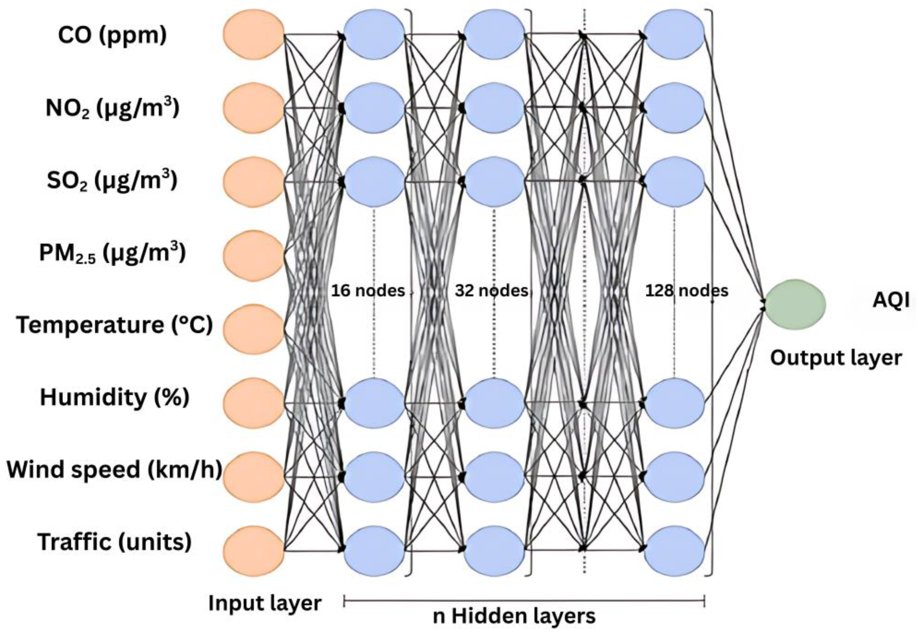
- Feedforward Neural Networks (FNNs) represent the most basic category of ANNs, characterized by non-cyclical node connections. In FNNs, data flow unidirectionally, moving from input nodes through any hidden nodes and ultimately reaching the output nodes. This architecture is specific for tasks where the relationship between input and output is straightforward and does not depend on previous inputs [85]. In this case, the hyperparameters that define the FNN architecture are nine dense layers (the first dense layer representing the network input layer), each dense layer having a specific number of neurons (respectively: 7, 8, 16, 32, 64, 128, 256, 256, 64), using Rectified Linear Unit (ReLu)-type activation function, one dropout layer to prevent overfitting (dropout rate 0.2), and one output layer (a dense one) with just one neuron, without activation function. Other hyperparameters are the employed optimizer was “Adam” with a learning rate of 0.001, the loss function for regression tasks was MSE, the number of epochs used for network training was set to 1000, batch size was 32, the validation split was set to 0.1 (10% of the data is used for validation during training), and the connections between layers are made in a feedforward manner (connected sequentially). The model parameters are the neurons connections weights (for instance, for the first dense layer) the weights shape is (1, 7), with associated weight matrix [0.618999, 0.47214946, 0.2781748, 0.753425, 0.06874061, 0.7170182, 0.35377005], and the bias for each neuron (for instance, the biases shape for the first dense layer) (7) and the corresponding biases vector is [−0.0030382, −0.00307668, 0.01217235, −0.00328257, −0.00333186, −0.00342433 0.00128003];
- Temporal Convolutional Networks (TCNs) utilize convolutional layers to process sequential data, offering an alternative to RNNs. TCNs are characterized by their ability to capture long-range dependencies through dilated convolutions, which allow for a larger receptive field without increasing the number of parameters [86]. The hyperparameters that define the TCNs architecture are: eight 1D Convolutional layers (the first layer representing the input layer-input shape, with a standard kernel size of 2 and causal type padding), each one with a specific number of output filters (4, 8, 16, 32, 64, 128, 256, 64) and ReLu-type activation function applied to each Conv1D layer, one dropout layer to prevent overfitting (dropout rate 0.2), one flatten layer used to transform the convolutional output into a one-dimensional vector, and an output layer (a dense one) with just one neuron. Another hyperparameter setup was as follows: the kernel size was set to 2, the number of filters was 4, 8, 16, 32, 64, 128, 256, 64 (increasing and then decreasing), the dilation rate was set to 1 for the first Conv1D layer and 2 for the rest of them, the dropout rate was 0.2, activation function was ReLu-type, the padding was “causal”. The hyperparameters learning rate for the “Adam” type optimizer, the loss function for regression tasks, the number of epochs used for network training, the batch size, the validation split, and the connections between layers were set to the same values as in the FNNs. The model parameters are the neurons connections weights (for instance, for the first Conv1D layer), weights of shape are (2, 1, 4) with associated weight matrix [[−0.585093, −0.42209578, −0.10097494, 0.88292724]; [−0.65418446, 0.56988806 0.11362608, 0.11557351]], and the bias for each neuron (for instance, the biases shape for the first Conv1D layer) is (4), and the corresponding biases vector is [0, 0.05134838, −0.0748504, 0.0022911];
- Recurrent Neural Networks (RNNs) handle sequential data by incorporating cycles in their architecture, allowing information to persist. This feature enables RNNs to maintain a form of memory. Standard RNNs face challenges with long-term dependencies because of problems such as vanishing and exploding gradients [87,88]. In this case, the hyperparameters that define the RNN architecture are three SimpleRNNs layers (the first one representing the input layer-input shape that defines the shape of the input data for the RNN layers, with 32 RNN units with a return sequence; the second one with 128 units with a return sequence and the third one with 256 units without a return sequence, the output of each RNN layer using ReLu-type activation function), a dropout layer to prevent overfitting with a dropout rate of 0.2, and an output layer (a dense one) with just one neuron. Other hyperparameters have the same values as those of FNNs and TCNs. The model parameters are the neurons connections weights (for instance, for the first SimpleRNNslayer) the weights shape is (1, 32) with associated weight matrix [−0.37684393, −0.3347999, 0.12421719, 0.04884235, 0.40717593, −0.2224836, 0.11467709, −0.44855782,…, 0.24549635, −0.4644161, 0.14050183, −0.421698, 0.4127007, 0.20661259, −0.17216238, −0.0187266], and the biases shape for each neuron (for instance, the biases shape for the first SimpleRNN layer) is (32) with the corresponding vector bias [0.20325282, 0.01771547, 0.27512175, …, 0.12933277, 0.10233897, −0.00640139];
- LSTMs are a form of RNN featuring memory cells and gating mechanisms that manage the flow of information. This architecture is used for tasks requiring the retention of information over extended periods, such as speech recognition and natural language processing [87,89,90]. In this case, the hyperparameters that describe this type of network architecture are two LSTM layers (the first LSTM layer contains the input shape, each one with 100 neurons, with ReLu-type used activation function, first LSTM layer with a return sequence and the second one without a return sequence), two dropout layers (with a dropout rate of 0.2 to prevent overfitting), and one output layer (a dense one, with just one neuron). Other hyperparameters have the same values as FNNs, TCNs, and RNNs. The model parameters are the neuron connection weights (for instance, for the last layer, the dense one), the weight matrix is (100, 1) (respectively, [[−0.1917704], …, [0.03949241]]), and the bias shape of the dense layer is (1), a 1D array ([0.34271002]).
- General Regression Neural Networks (GRNNs) are FNNs designed for regression tasks. They utilize a kernel-based approach to estimate the output for a given input, used for problems where the relationship between input and output is not strictly linear [85,91]. The hyperparameters that define the FNN architecture are five dense layers (hidden layers—dense ones, the first one representing the input layer with 64 units, the second one with 128 units, the third and the fourth layer with 256 units, and the fifth layer with 64 units, all dense layers using Radial Basis Function (RBF) activation function), one dropout layer to prevent overfitting with dropout rate 0.2 and, and an output layer (a dense one) with just one neuron. Other hyperparameters have the same values as FNNs, TCNs, RNNs, and LSTMs. Regarding the parameters, the important ones are the neurons connections weights (for instance, for the first dense layer) weight shape is (64, 128) with the corresponding weights matrix ([[0.09693588, 0.11530785, 0.04327405, …, −0.01015339, −0.00465284, −0.16290204], …, [0.18151447, −0.00127745, 0.11786038, …, −0.06098074, 0.0883746, −0.14132085]]) and bias shape (for the same first dense layer) that is (128), with the corresponding bias array [0.01425829, −0.019097, 0.02077781, 0.05533804, −0.02579543, −0.05466483, …, 0.03854505, −0.08813311, −0.0760707, 0.03319431, −0.03673444, −0.02343925, −0.01249062, −0.04072443].
- Time-Delay Neural Networks (TDNNs) are designed to process temporal data by incorporating delays in the input layer. This architecture allows TDNNs to adapt unstructured data speech recognition, image processing, and time series analysis [92]. In this case, the hyperparameters that define the TDNN architecture are an input layer (the input shape that is determined by the number of the time step and the number of features in the training data), five hidden layers (dense ones, first one with 64 units, second one with 128 units, the third and the fourth one with 256 units, and the fifth one with 64 units, each one using ReLu-type activation function), a dropout layer to prevent overfitting (dropout rate of 0.2), a flatten layer used to convert the output of the last dense layer to a one-dimensional vector necessary for the output layer and, one output layer with just one unit (a dense one). Other hyperparameters are the same and with the same values as in the case of FNNs, TCNs, RNNs, LSTMs, and GRNNs, to which it is added the number of time steps (time_steps) that was set to 4. Regarding the model parameters, for instance, for the first dense layer, the weights of the shape are (64, 128) with the associated matrix weights ([[−0.18985237, −0.23790528, −0.26162702, …, −0.21098962, −0.34780186, 0.00897838], …, [0.23329817, −0.03779398, 0.08295902 … −0.13313578, 0.11072736, −0.10848673]]) and biases shape (128), with the associated biases 1D array [−6.65585697 × 10⁻², 2.33586300 × 10⁻², −8.02270137 × 10⁻³, −6.08175024 × 10⁻², …, −3.14048007 × 10⁻², −1.27918571 × 10⁻¹, −8.52884054 × 10⁻², −2.51952391 × 10⁻²].
- Deep Belief Networks (DBNs) are associated with complex hierarchical data representations. DBNs capture intricate relationships between features and the AQI for AQ prediction, improving forecasting performance [93,94]. This type of network architecture presents the next hyperparameters: an input layer (that corresponds to the number of features in the dataset), a sequence of autoencoders that successively apply transformations to the data, each one encoding previous data representations, respectively, four encoding layers that perform data compression (dense ones, with ReLu-type activation function), one decoding layer to reconstruct the input data (a dense one, with “sigmoid” type activation function), one dropout layer to prevent overfitting (dropout rate 0.2), and an output layer (a dense one, with just one unit). Other hyperparameters are the same and with the same values as in the case of FNNs, TCNs, RNNs, LSTMs, and GRNNs, to which added the data autoencoders encoding dimensions that are [1024, 64, 512, 32], the autoencoders training (number of epochs for autoencoders training was set to 50, batch size 32 and, the validation split was set to 0.1). Regarding the model parameters, for instance, for the second layer (first encoder layer of the autoencoder) the weights shape is (1024, 64) with the corresponding matrix weights [[−0.01099487, 0.05026998, −0.04905977, …, −0.06741306, 0.15472981, −0.25435853], …, [−0.04147308, −0.02906811, −0.00823338, …, −0.05285922, −0.1270246, −0.180068 ]] and biases shape is (64) with the corresponding bias vector [−0.02391353, −0.0217452, −0.02374031, −0.02275715, −0.00915561, −0.02361129, …, −0.02615629, −0.0149049, −0.0102234, −0.08077513].
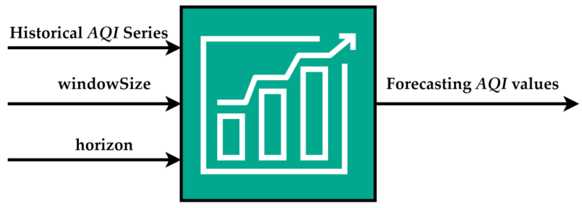
2.4. Forecasting Algorithm for AQI
- The input column contains the historical AQI values used to train the model. The accuracy of predictions relies on the quality and quantity of the historical data between 1 January 2020 and 31 December 2023;
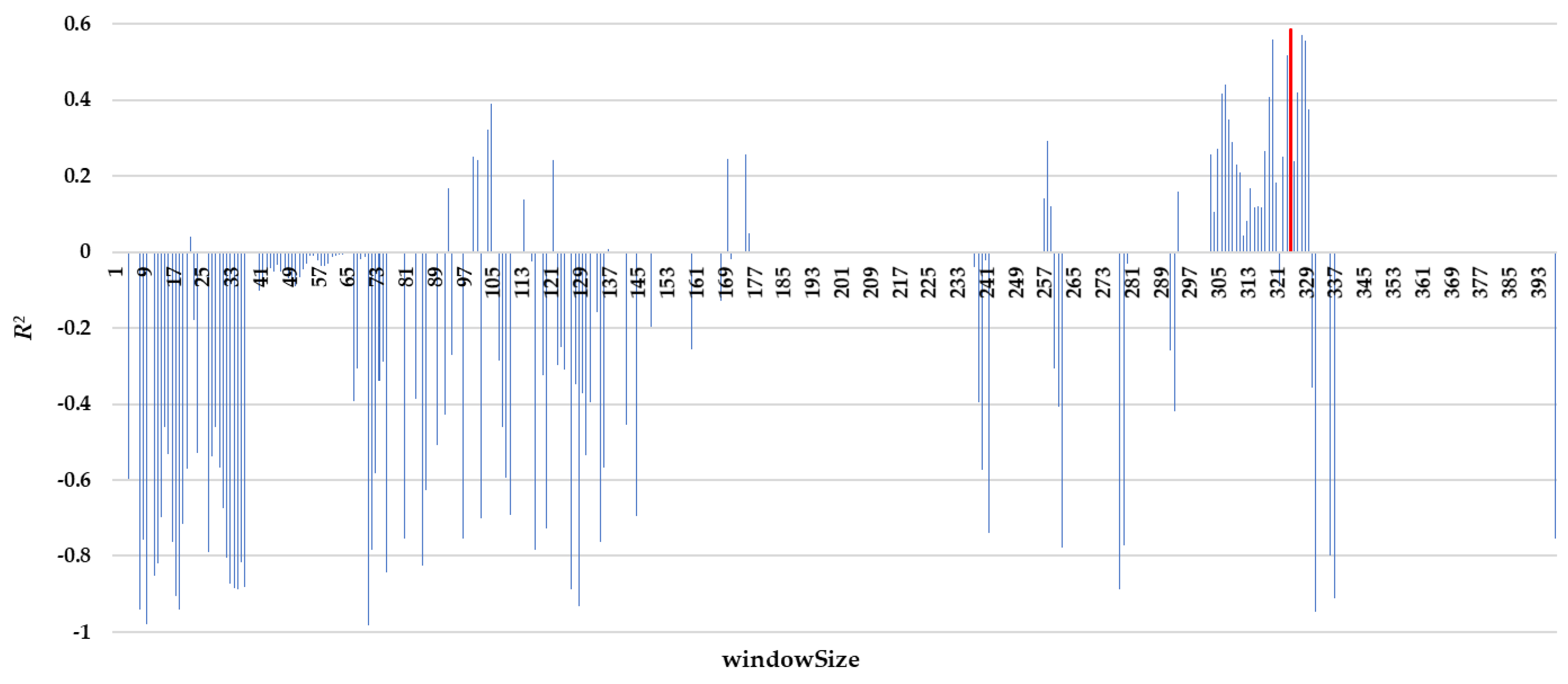
- The windowSize determines how many past observations are considered to predict future values. Multiple tests were provided for this parameter to obtain the best value for the accuracy of the forecasting;
- The horizon parameter specifies how many future days the model will forecast. This value is set to 5 days;
- The output column contains the forecasted AQI values for the next five days, predicted after the model is trained. These values are displayed in the proposed environmental monitoring and public health application.
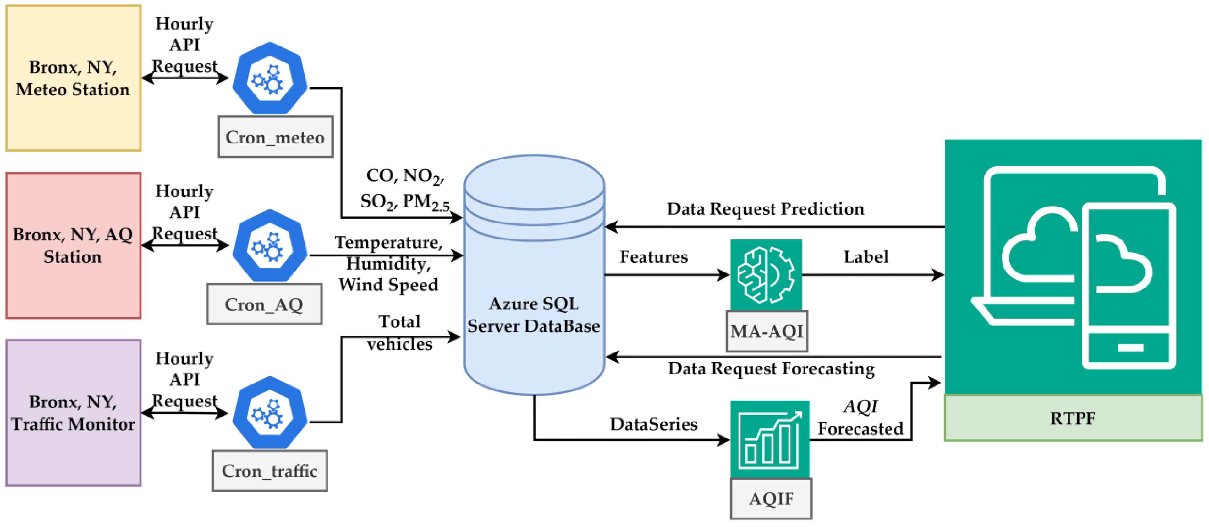
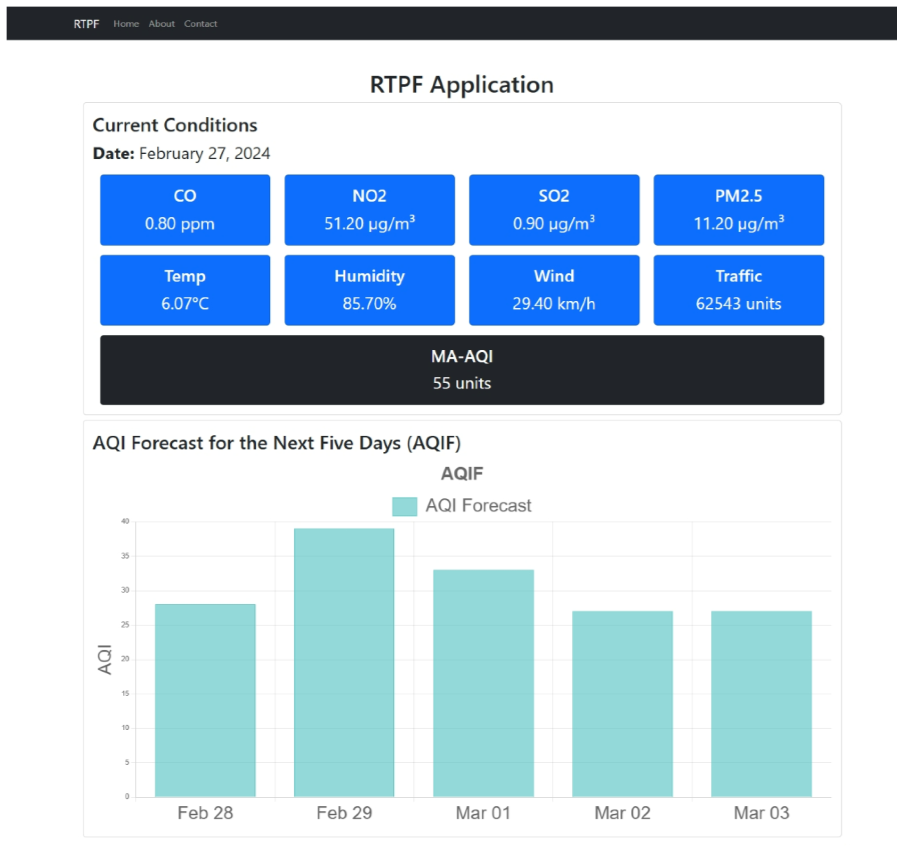
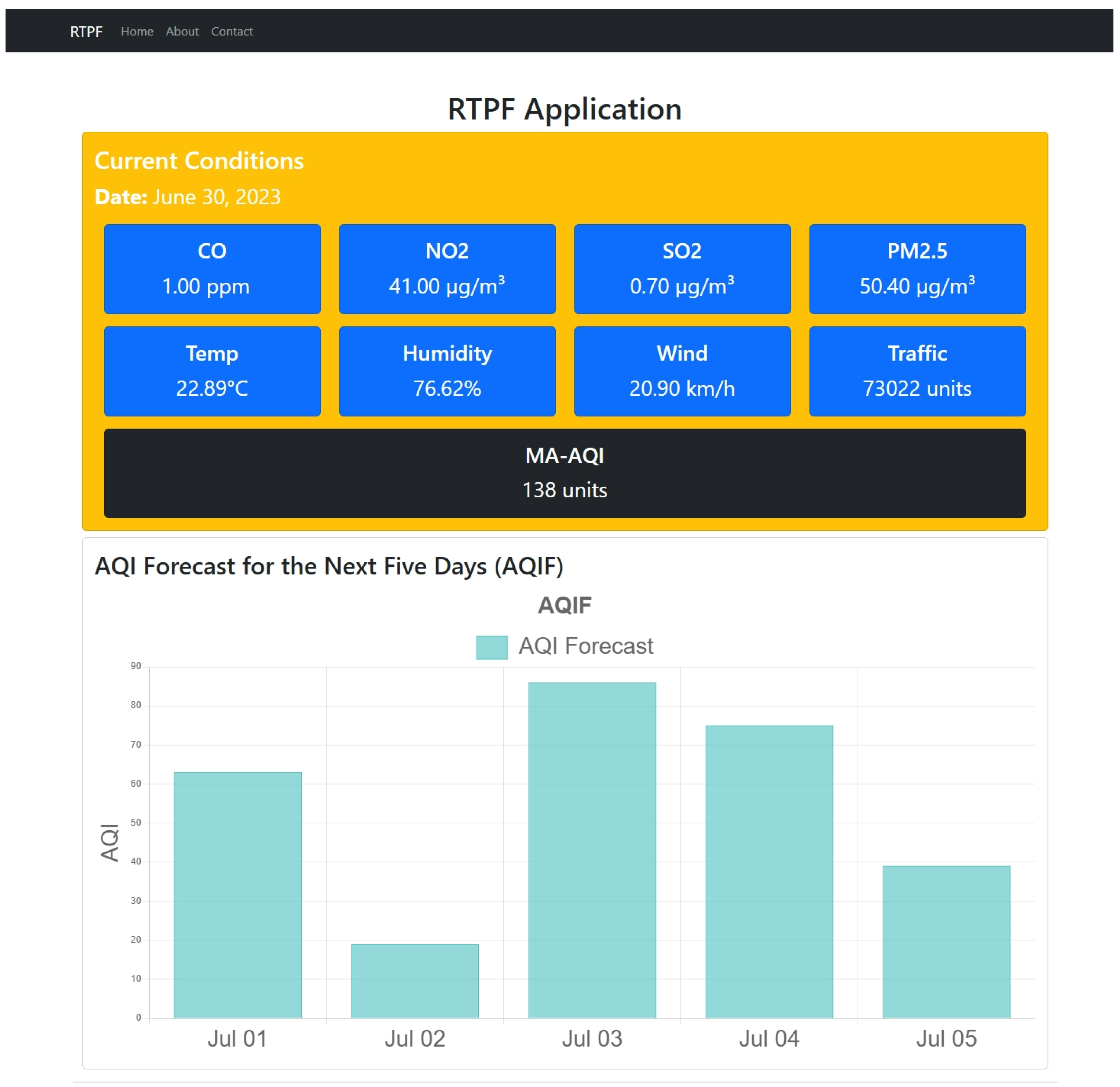
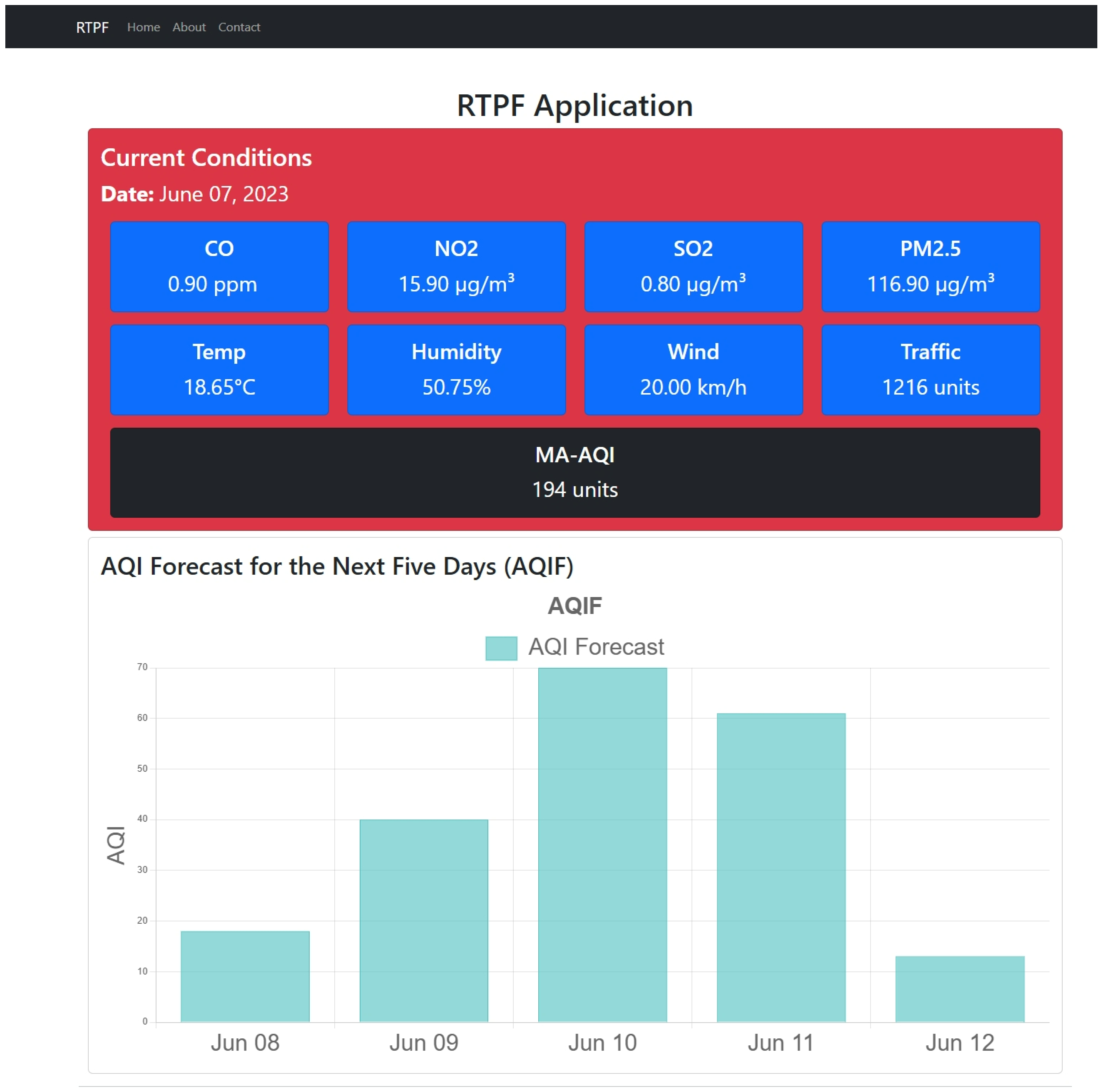
2.5. Real-Time Prediction and Forecasting Application
- The locally trained MA-AQI and AQIF models need to be hosted in the cloud to ensure they are accessible;
- A reliable data acquisition system must be established to use real-time data as inputs for the MA-AQI model. This involves collecting data from various sensors and devices and centralizing it within an IoT infrastructure. There are two primary approaches to achieve this:
- ○
- Data can be entered into a cloud-hosted database via API requests. This method facilitates data storage and retrieval while ensuring that the information remains up-to-date and accessible for analysis;
- ○
- Another solution involves employing an IoT hub service like Azure IoT Hub. This service platform connects IoT devices, enabling real-time data ingestion, management, and analysis.
- Data Collection Sources:
- Meteo Station. This component retrieves hourly data on weather parameters. The data are collected via an API when the cron job Cron_meteo runs hourly on the API. The result produced by the API is sent to the SQL Server Database hosted in Azure Cloud;
- AQ Station. AQ parameters such as CO, NO2, SO2, and PM2.5 are gathered from the AQ monitoring station. These data are also transmitted via an API to the central database hourly when the Cron_AQ job is executed;
- Traffic Monitor. The number of vehicles is collected in real-time through an API and sent to the Azure SQL Server when the Cron_traffic hourly execution is released.
- The central repository Azure SQL Server Database receives and stores all the data from the three primary sources (Meteo Station, AQ Station, and Traffic Monitor). The stored data include air pollutants, weather conditions, and traffic information, which the prediction and forecasting models then utilize.
- The MA-AQI model’s prediction receives the collected features (pollutant levels, weather data, and traffic counts) from the Azure SQL Database and predicts the AQI as the label. This is used to determine the current state of AQ based on the data inputs.
- Forecasting Model AQIF forecasts the future AQI based on historical data series from the Azure SQL Database. It predicts the future AQI trend, potentially for proactive measures or alerts.
- RTPF collects the predicted AQI from MA-AQI and the forecasted AQI from AQIF. This platform provides a real-time dashboard where users view the current and predicted AQ data on different devices (laptops, tablets, or mobile devices).
- Data Integration. All collected environmental and traffic data are integrated into a central Azure SQL Server database for further processing;
- Real-Time Prediction. The system predicts current AQI based on real-time data using the MA-AQI model;
- Forecasting. The system forecasts future AQI trends using historical data.
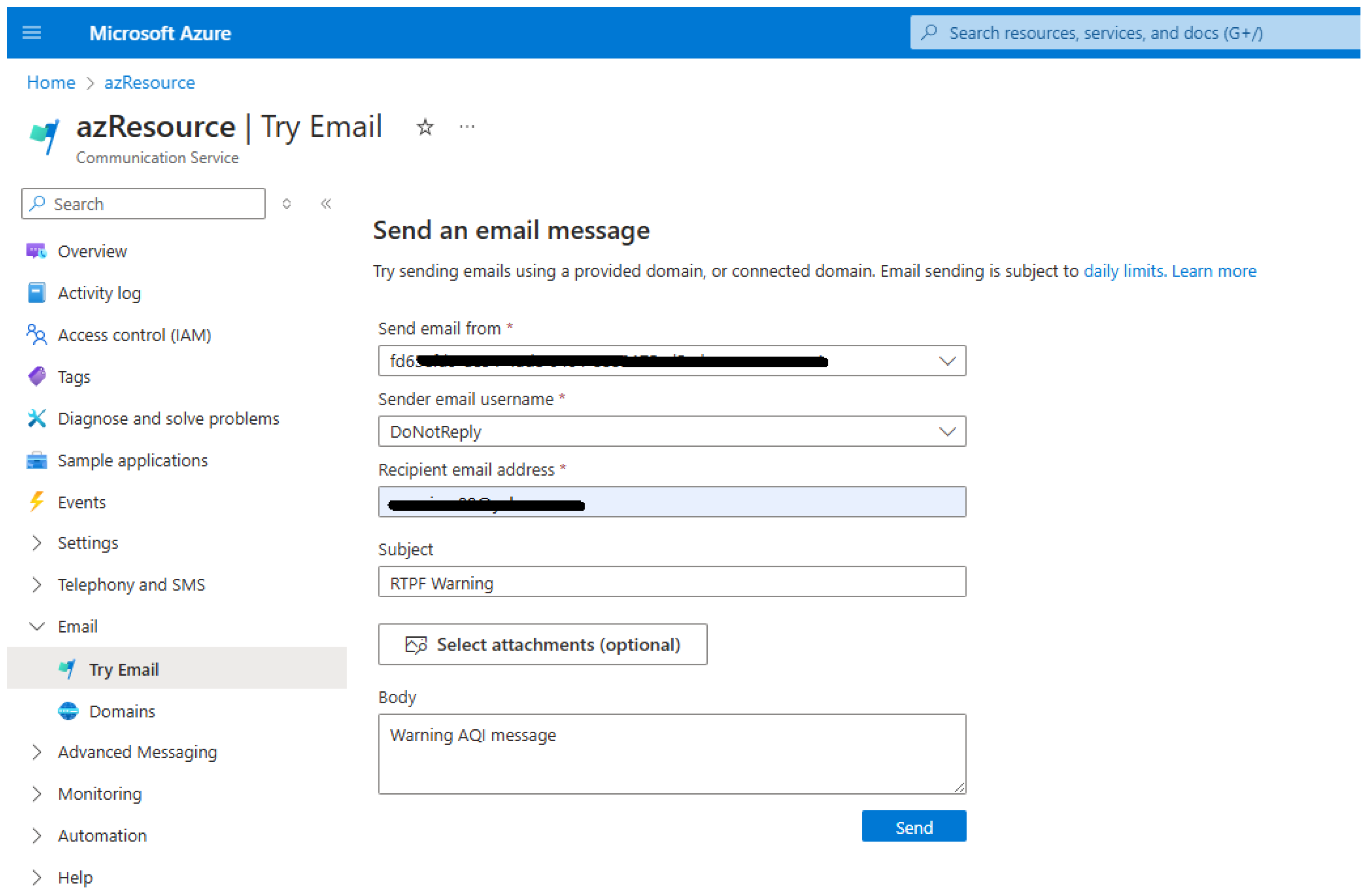
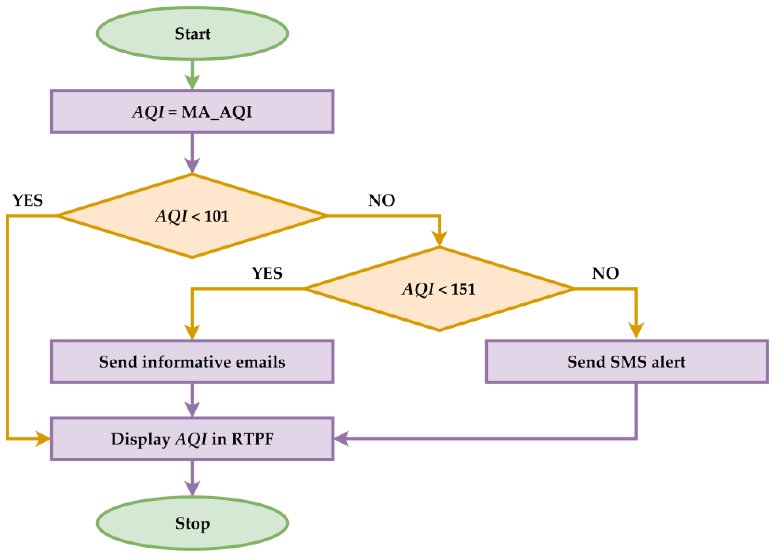
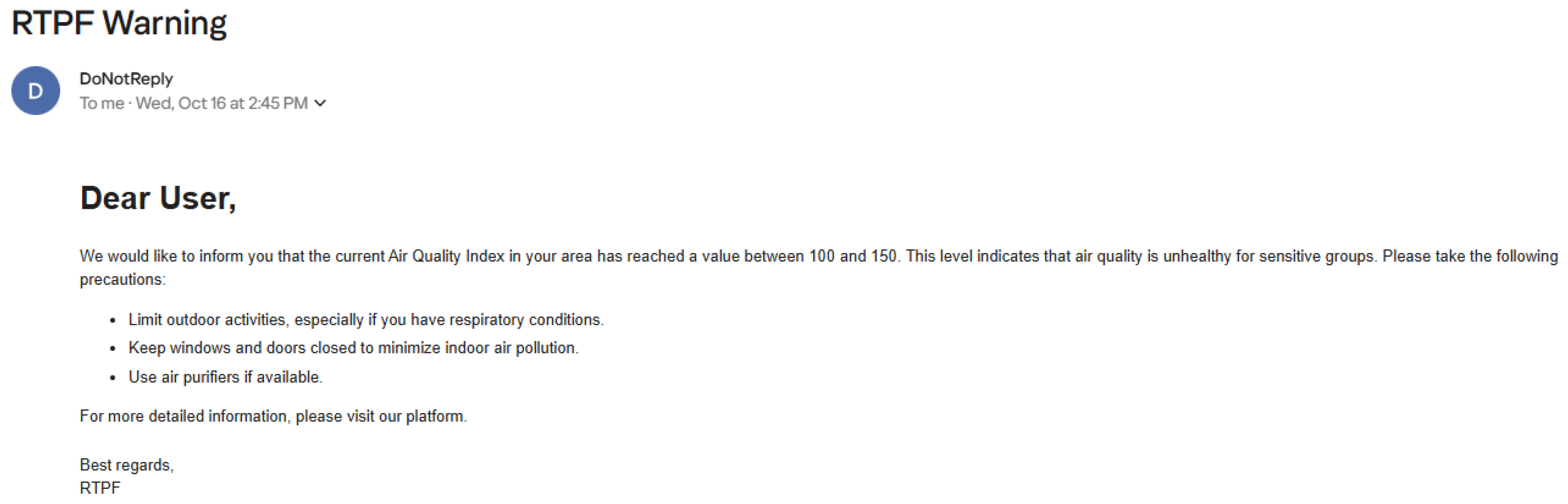
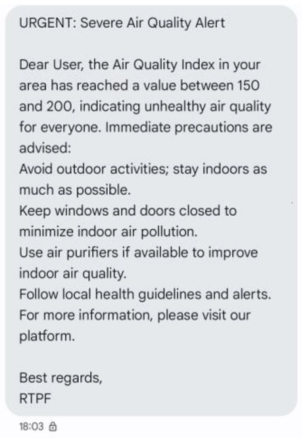
2.6. Emergency Response Protocol Integration for Exceeding Safe AQI Levels
3. Results
3.1. ML and DL Model Results
- For each customized DL algorithm (unlike the original algorithm), a dropout layer was added that ignores twenty percent of the data for network overfitting prevention, and in the case of some algorithms (for instance, for RNNs and LSTMs) was integrated a return sequence for better performances. Also, the input layer (the input shape) for some types of networks (for instance, for FNNs and GRNNs) was integrated into the network-dense layers. In contrast, for TCNs, the input shape was incorporated into the convolutional layers, with a standard kernel size of 2 and a causal type padding;
- For each customized DL algorithm, the number of layers (dense layers) of densely interconnected nodes (that are using ReLu or RBF), the number of nodes for each layer (for instance, FNNs contain nine layers of densely interconnected nodes that start at seven nodes and doubles in number up to two hundred and fifty-six nodes), the number of 1D Convolutional layers (for TCNs) that supplies the output filter starting from a number of four nodes to a number of two hundred and fifty-six nodes, and the number of flattening layers (for TCNs, such a layer being used to flatten the output to the correct size) were established. Also, the number of SimpleRNN layers (for RNNs, where the first layer contains thirty-two nodes with a return sequence, the second one has one hundred and twenty-eight nodes with a return sequence, and the third one includes two hundred and fifty-six nodes without a return sequence), the number of final layers that contains just one output (for instance, for DBNs and TCNs), and the number of layers of autoencoders (for example, for DBNs).
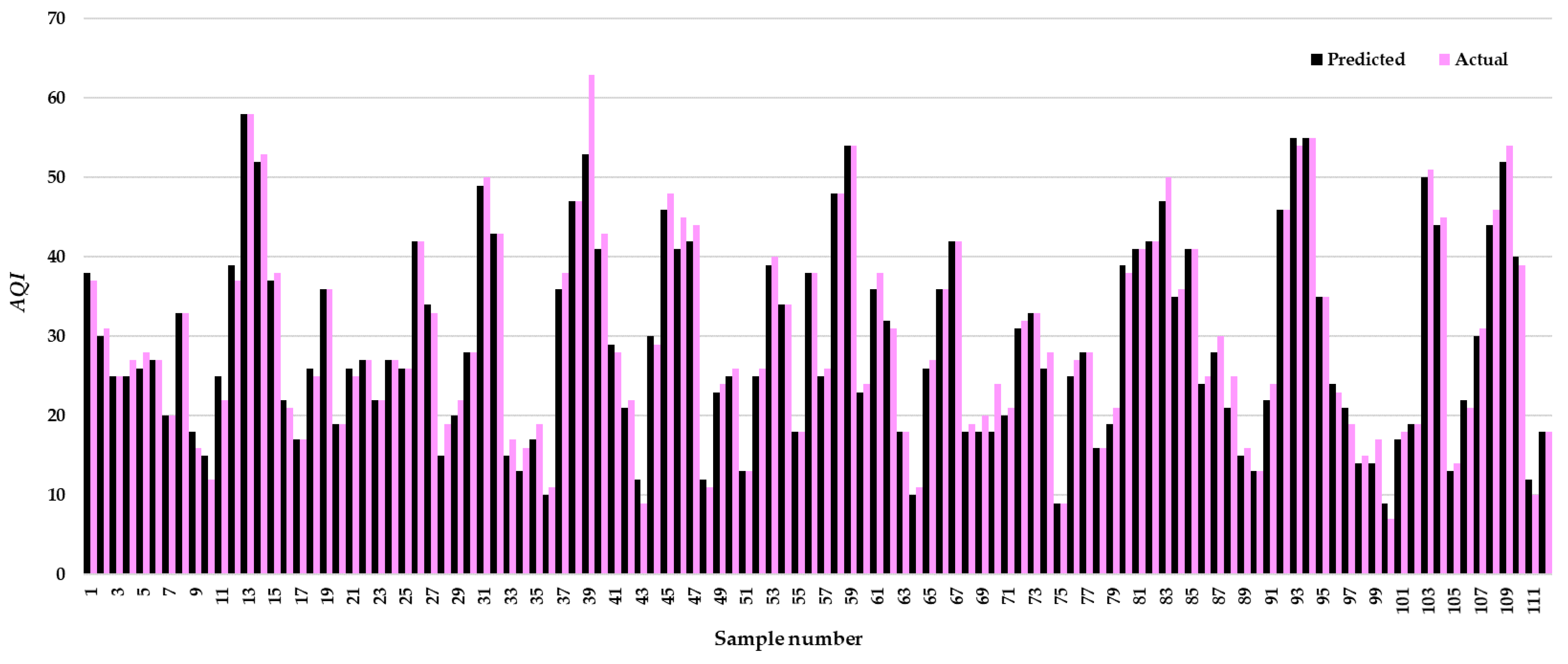
3.2. Model Validation
3.3. Forecasting Model Results
3.4. PIP Warnings and Alerts
4. Discussion
5. Conclusions
Supplementary Materials
Author Contributions
Funding
Institutional Review Board Statement
Informed Consent Statement
Data Availability Statement
Conflicts of Interest
Abbreviations
| % | Percentage |
| µg/m3 | Micrograms per cubic meter |
| ADAM | Adaptive Moment Estimation |
| AI | Artificial intelligence |
| AIS | Automatic Identification System |
| ANN | Artificial neural network |
| AQ | Air quality |
| AQI | Air quality index |
| AQIF | Air Quality Index Forecasting |
| AQMS | Air quality monitoring system |
| CNN | Convolutional neural network |
| CO | Carbon monoxide |
| DBN | Deep Belief Network |
| DL | deep learning |
| DTR | Decision Tree Regression |
| EPA | Environmental Protection Agency |
| FNN | Feedforward Neural Network |
| GAM | Generalized Additive Models |
| GBR | Gradient Boosting Regression |
| GRNN | General Regression Neural Network |
| GSM | Global System for Mobile Communications |
| GUI | Graphical user interface |
| IoT | Internet of Things |
| km/h | kilometers per hour |
| KNN | K-nearest neighbors |
| LR | Linear Regression |
| LSTM | Long Short-Term Memory |
| MA-AQI | Most accurate model for predicting AQI |
| MAE | Mean Absolute Error |
| MAPE | Mean Absolute Percentage Error |
| MedAE | Median Absolute Error |
| ML | Machine learning |
| MSE | Mean squared error |
| NO2 | Nitrogen dioxide |
| O3 | Ozone |
| OMAP | Open Meteo API Portal |
| OP | Overall precision |
| PIP | Proposed intervention protocols |
| PM | Particulate matter |
| PM10 | Particulate matter with diameters of 10 µm and smaller |
| PM2.5 | Particulate matter with diameters of 2.5 µm and smaller |
| ppm | Parts per million |
| RAQP | Recurrent air quality predictor |
| RBF | Radial Basis Function |
| ReLu | Rectified Linear Unit |
| RFR | Random Forest Regression |
| RMSE | Root mean square error |
| RNN | Recurrent neural network |
| RTPF | Real-Time Prediction and Forecasting |
| SMS | Short Message Service |
| SO2 | Sulfur dioxide |
| SVR | Support Vector Regression |
| TCN | Temporal Convolutional Network |
| TDNN | Time-Delay Neural Network |
| VOC | Volatile organic compound |
References
- Munfarida, I.; Arida, V. Air Pollution Assessment in the Main Roads of Surabaya-Indonesia During Post COVID-19. Int. J. Environ. Sustain. Soc. Sci. 2023, 4, 664–671. [Google Scholar] [CrossRef]
- Chong, C. Carbon Monoxide Pollution and Limited Health Service Access in Third-world Countries. J. Glob. Ecol. Environ. 2024, 20, 17–27. [Google Scholar] [CrossRef]
- Rosca, C.-M.; Stancu, A.; Neculaiu, C.-F.; Gortoescu, I.-A. Designing and Implementing a Public Urban Transport Scheduling System Based on Artificial Intelligence for Smart Cities. Appl. Sci. 2024, 14, 8861. [Google Scholar] [CrossRef]
- Panait, M.; Voica, M.C.; Rădulescu, I. Approaches Regarding Environmental Kuznets Curve in the European Union from the Perspective of Sustainable Development. Appl. Ecol. Environ. Res. 2009, 17, 6801–6820. [Google Scholar] [CrossRef]
- Wang, Y.; Li, C.; Ruan, Z.; Ye, R.; Yang, B.; Ho, H.C. Effects of Ambient Exposure to Nitrogen Dioxide on Outpatient Visits for Psoriasis in Rapidly Urbanizing Areas. Aerosol Air Qual. Res. 2022, 22, 220166. [Google Scholar] [CrossRef]
- Zhang, Y.; Yang, D.; Wu, R.; Li, Y.; Yang, X.; Wang, R.; Xu, H. Characterization of roadside air pollutants: An artery road of Lanzhou city in northwest China. In Proceedings of the 8th International Symposium on Vehicle Emission Supervision and Environment Protection, Wuhan, China, 23–24 June 2022; p. 01039. [Google Scholar] [CrossRef]
- Srivastava, S.; Kumar, A.; Bauddh, K.; Gautam, A.S.; Kumar, S. 21-Day Lockdown in India Dramatically Reduced Air Pollution Indices in Lucknow and New Delhi, India. Bull. Environ. Contam. Toxicol. 2020, 105, 9–17. [Google Scholar] [CrossRef]
- Rendana, M.; Komariah, L.N. The relationship between air pollutants and COVID-19 cases and its implications for air quality in Jakarta, Indonesia. J. Pengelolaan Sumberd. Alam Dan Lingkung. 2021, 11, 93–100. [Google Scholar] [CrossRef]
- Olmo, N.R.S.; Do Nascimento Saldiva, P.H.; Braga, A.L.F.; Lin, C.A.; De Paula Santos, U.; Pereira, L.A.A. A review of low-level air pollution and adverse effects on human health: Implications for epidemiological studies and public policy. Clinics 2011, 66, 681–690. [Google Scholar] [CrossRef]
- Rosca, C.M.; Popescu, M.; Patrascioiu, C.; Stancu, A. Comparative Analysis of pH Level Between Pasteurized and UTH Milk Using Dedicated Developed Application. Rev. Chim. 2019, 70, 3917–3920. [Google Scholar] [CrossRef]
- Anwar, M.Z.; Rindarjono, M.G.; Ahmad. The impact of transportation growth on the increase SO2 and NO2 gases in Surakarta City during 2013–2020. In Proceedings of the International Conference on Anthropocene, Global Environmental Change and Powerful Geography, Online, Indonesia, 27 September 2022; p. 012028. [Google Scholar] [CrossRef]
- Wyche, K.P.; Nichols, M.; Parfitt, H.; Beckett, P.; Gregg, D.J.; Smallbone, K.L.; Monks, P.S. Changes in ambient air quality and atmospheric composition and reactivity in the South East of the UK as a result of the COVID-19 lockdown. Sci. Total Environ. 2021, 755, 142526. [Google Scholar] [CrossRef]
- Apostu, S.A.; Gigauri, I.; Panait, M.; Martín-Cervantes, P.A. Is Europe on the Way to Sustainable Development? Compatibility of Green Environment, Economic Growth, and Circular Economy Issues. Int. J. Environ. Res. Public Health 2023, 20, 1078. [Google Scholar] [CrossRef] [PubMed]
- Stancu, A. Impact of COVID-19 Pandemic on International Agricultural Trade in European Countries. In Shifting Patterns of Agricultural Trade; Erokhin, V., Tianming, G., Andrei, J.V., Eds.; Springer: Singapore, 2021; pp. 263–284. [Google Scholar] [CrossRef]
- Akan, A.P.; Coccia, M. Changes of Air Pollution between Countries Because of Lockdowns to Face COVID-19 Pandemic. Appl. Sci. 2022, 12, 12806. [Google Scholar] [CrossRef]
- Alzayed, M.A.; Aljame, M.; Ahmad, I. Investigating the impact of COVID-19 lockdowns on environmental health in Kuwait. J. Eng. Res. 2023, 11, 317–328. [Google Scholar] [CrossRef]
- Sarmadi, M.; Rahimi, S.; Rezaei, M.; Sanaei, D.; Dianatinasab, M. Air quality index variation before and after the onset of COVID-19 pandemic: A comprehensive study on 87 capital, industrial and polluted cities of the world. Environ. Sci. Eur. 2021, 33, 134. [Google Scholar] [CrossRef] [PubMed]
- Schiavo, B.; Morton-Bermea, O.; Arredondo-Palacios, T.E.; Meza-Figueroa, D.; Robles-Morua, A.; García-Martínez, R.; Valera-Fernández, D.; Inguaggiato, C.; Gonzalez-Grijalva, B. Analysis of COVID-19 Lockdown Effects on Urban Air Quality: A Case Study of Monterrey, Mexico. Sustainability 2022, 15, 642. [Google Scholar] [CrossRef]
- Benchrif, A.; Wheida, A.; Tahri, M.; Shubbar, R.M.; Biswas, B. Air quality during three COVID-19 lockdown phases: AQI, PM2.5 and NO2 assessment in cities with more than 1 million inhabitants. Sustain. Cities Soc. 2021, 74, 103170. [Google Scholar] [CrossRef]
- Keller, C.A.; Evans, M.J.; Knowland, K.E.; Hasenkopf, C.A.; Modekurty, S.; Lucchesi, R.A.; Oda, T.; Franca, B.B.; Mandarino, F.C.; Díaz Suárez, M.V.; et al. Global impact of COVID-19 restrictions on the surface concentrations of nitrogen dioxide and ozone. Atmos. Chem. Phys. 2021, 21, 3555–3592. [Google Scholar] [CrossRef]
- Jacob, D.; Stowe, S.; Babarinde, I.; Sharma, A.; Christopher, A.; Vilcassim, M.J.R. The Impact of COVID-19 Related Changes on Air Quality in Birmingham, Alabama, United States. Int. J. Environ. Res. Public Health 2022, 19, 3168. [Google Scholar] [CrossRef]
- Rosca, C.M. Convergence Catalysts: Exploring the Fusion of Embedded Systems, IoT, and Artificial Intelligence. In Engineering Applications of AI and Swarm Intelligence; Yang, X.-S., Ed.; Springer Nature: Singapore, 2025; pp. 69–87. [Google Scholar] [CrossRef]
- Rosca, C.M.; Gortoescu, I.A.; Tanase, M.R. Artificial Intelligence—Powered Video Content Generation Tools. Rom. J. Pet. Gas Technol. 2024, V (LXXVI), 131–144. [Google Scholar] [CrossRef]
- Waseem, K.H.; Mushtaq, H.; Abid, F.; Abu-Mahfouz, A.M.; Shaikh, A.; Turan, M.; Rasheed, J. Forecasting of Air Quality Using an Optimized Recurrent Neural Network. Processes 2022, 10, 2117. [Google Scholar] [CrossRef]
- Tao, Q.; Liu, F.; Li, Y.; Sidorov, D. Air Pollution Forecasting Using a Deep Learning Model Based on 1D Convnets and Bidirectional GRU. IEEE Access 2019, 7, 76690–76698. [Google Scholar] [CrossRef]
- Zhang, T.; Dick, R.P. Image-Based Air Quality Forecasting Through Multi-Level Attention. In Proceedings of the IEEE International Conference on Image Processing, Bordeaux, France, 16–19 October 2022; pp. 686–690. [Google Scholar] [CrossRef]
- Murad, A.; Kraemer, F.A.; Bach, K.; Taylor, G. Probabilistic Deep Learning to Quantify Uncertainty in Air Quality Forecasting. Sensors 2021, 21, 8009. [Google Scholar] [CrossRef]
- Kodak, G. An Investigation on the Use of Air Quality Models in Ship Emission Forecasts. J. Intell. Transp. Syst. Appl. 2024, 7, 15–30. [Google Scholar] [CrossRef]
- Weissert, L.F.; Alberti, K.; Miskell, G.; Pattinson, W.; Salmond, J.A.; Henshaw, G.; Williams, D.E. Low-cost sensors and microscale land use regression: Data fusion to resolve air quality variations with high spatial and temporal resolution. Atmos. Environ. 2019, 213, 285–295. [Google Scholar] [CrossRef]
- Wang, D.; Wang, H.-W.; Lu, K.-F.; Peng, Z.-R.; Zhao, J. Regional Prediction of Ozone and Fine Particulate Matter Using Diffusion Convolutional Recurrent Neural Network. Int. J. Environ. Res. Public Health 2022, 19, 3988. [Google Scholar] [CrossRef]
- Rosca, C.-M.; Stancu, A. Earthquake Prediction and Alert System Using IoT Infrastructure and Cloud-Based Environmental Data Analysis. Appl. Sci. 2024, 14, 10169. [Google Scholar] [CrossRef]
- Sekula, P.; Ustrnul, Z.; Bokwa, A.; Bochenek, B.; Zimnoch, M. Random Forests Assessment of the Role of Atmospheric Circulation in PM10 in an Urban Area with Complex Topography. Sustainability 2022, 14, 3388. [Google Scholar] [CrossRef]
- Vu, T.V.; Shi, Z.; Cheng, J.; Zhang, Q.; He, K.; Wang, S.; Harrison, R.M. Assessing the impact of clean air action on air quality trends in Beijing using a machine learning technique. Atmos. Chem. Phys. 2019, 19, 11303–11314. [Google Scholar] [CrossRef]
- Hamami, F.; Dahlan, I.A. Air Quality Classification in Urban Environment using Machine Learning Approach. In Proceedings of the International Conference on Disaster Management and Climate Change, Surakarta, Indonesia, 9 April 2021; p. 012004. [Google Scholar] [CrossRef]
- Badrakh, O.; Choimaa, L. Air quality predictions of Ulaanbaatar using machine learning approach. In Proceedings of the International Symposium on Grids & Clouds, Taipei, Taiwan, 22–26 March 2021; pp. 1–7. [Google Scholar] [CrossRef]
- Du, S.; Li, T.; Yang, Y.; Horng, S.-J. Deep Air Quality Forecasting Using Hybrid Deep Learning Framework. IEEE Trans. Knowl. Data Eng. 2021, 33, 2412–2424. [Google Scholar] [CrossRef]
- Huang, C.-J.; Kuo, P.-H. A Deep CNN-LSTM Model for Particulate Matter (PM2.5) Forecasting in Smart Cities. Sensors 2018, 18, 2220. [Google Scholar] [CrossRef]
- Liu, Y.; Wang, P.; Li, Y.; Wen, L.; Deng, X. Air quality prediction models based on meteorological factors and real-time data of industrial waste gas. Sci. Rep. 2022, 12, 9253. [Google Scholar] [CrossRef]
- Akdi, Y.; Gölveren, E.; Ünlü, K.D.; Yücel, M.E. Modeling and forecasting of monthly PM2.5 emission of Paris by periodogram-based time series methodology. Environ. Monit. Assess. 2021, 193, 622. [Google Scholar] [CrossRef] [PubMed]
- Rosca, C.-M.; Stancu, A.; Popescu, M. The Impact of Cloud Versus Local Infrastructure on Automatic IoT-Driven Hydroponic Systems. Appl. Sci. 2025, 15, 4016. [Google Scholar] [CrossRef]
- Liu, Q.; Cui, B.; Liu, Z. Air Quality Class Prediction Using Machine Learning Methods Based on Monitoring Data and Secondary Modeling. Atmosphere 2024, 15, 553. [Google Scholar] [CrossRef]
- Fang, L.; Jin, J.; Segers, A.; Lin, H.X.; Pang, M.; Xiao, C.; Deng, T.; Liao, H. Development of a regional feature selection-based machine learning system (RFSML v1.0) for air pollution forecasting over China. Geosci. Model Dev. 2022, 15, 7791–7807. [Google Scholar] [CrossRef]
- IQAir. Air Quality in The Bronx. Available online: https://www.iqair.com/us/usa/new-york/the-bronx (accessed on 10 April 2025).
- Rosca, C.M.; Stancu, A.; Ariciu, A.V. Algorithm for child adoption process using artificial intelligence and monitoring system for children. Internet Things 2024, 26, 101170. [Google Scholar] [CrossRef]
- Bajpai, A.; Girish Kumar, T.P.; Sreenivasan, G.; Srivastav, S.K. System Design, Automatic Data Collection Framework and Embedded Software Development of Internet of Things (IoT) for Air Pollution Monitoring of Nagpur Metropolis. J. Indian Soc. Remote Sens. 2024, 52, 2347–2359. [Google Scholar] [CrossRef]
- Martín-Baos, J.Á.; Rodriguez-Benitez, L.; García-Ródenas, R.; Liu, J. IoT based monitoring of air quality and traffic using regression analysis. Appl. Soft Comput. 2022, 115, 108282. [Google Scholar] [CrossRef]
- Shahid, I.; Shahzad, M.I.; Tutsak, E.; Mahfouz, M.M.K.; Al Adba, M.S.; Abbasi, S.A.; Rathore, H.A.; Asif, Z.; Chen, Z. Carbon based sensors for air quality monitoring networks; middle east perspective. Front. Chem. 2024, 12, 1391409. [Google Scholar] [CrossRef]
- Kumar, Y.J.N.; Chandan, R.; Somanini, S.H.; Vadtya, S.; Dangi, D. Ecosense: An IoT System for Detecting Suitable and Sustainable Living Conditions. In Proceedings of the 15th International Conference on Materials Processing and Characterization, Newcastle, UK, 5–8 September 2023; p. 01085. [Google Scholar] [CrossRef]
- Marques, G.; Pitarma, R. A Cost-Effective Air Quality Supervision Solution for Enhanced Living Environments through the Internet of Things. Electronics 2019, 8, 170. [Google Scholar] [CrossRef]
- Jo, J.; Jo, B.; Kim, J.; Kim, S.; Han, W. Development of an IoT-Based Indoor Air Quality Monitoring Platform. J. Sens. 2020, 2020, 749764. [Google Scholar] [CrossRef]
- Rosca, C.-M.; Stancu, A. A Comprehensive Review of Machine Learning Models for Optimizing Wind Power Processes. Appl. Sci. 2025, 15, 3758. [Google Scholar] [CrossRef]
- Shrestha, R.; Maharjan, M.; Sharma, M. Air Pollution Monitoring System Using Micro Controller Atmega 32A and MQ135 Gas Sensor at Chandragiri Municipality of Kathmandu City. Semicond. Sci. Inf. Devices 2022, 4, 35–44. [Google Scholar] [CrossRef]
- Zheng, T.; Bergin, M.H.; Johnson, K.K.; Tripathi, S.N.; Shirodkar, S.; Landis, M.S.; Sutaria, R.; Carlson, D.E. Field evaluation of low-cost particulate matter sensors in high- and low-concentration environments. Atmos. Meas. Tech. 2018, 11, 4823–4846. [Google Scholar] [CrossRef]
- Cowell, N.; Chapman, L.; Bloss, W.; Srivastava, D.; Bartington, S.; Singh, A. Particulate matter in a lockdown home: Evaluation, calibration, results and health risk from an IoT enabled low-cost sensor network for residential air quality monitoring. Environ. Sci. Atmos. 2023, 3, 65–84. [Google Scholar] [CrossRef]
- Rosca, C.-M.; Stancu, A.; Tănase, M.R. A Comparative Study of Azure Custom Vision Versus Google Vision API Integrated into AI Custom Models Using Object Classification for Residential Waste. Appl. Sci. 2025, 15, 3869. [Google Scholar] [CrossRef]
- Tooki, O.O.; Tamasi, M.A.; Ohemu, M.F.; Ogunkeyede, O.Y.; Abolade, R.O. Implementation of a sustainable real-time air quality monitoring system using the Internet of Things for Kaduna metropolis, Nigeria. LAUTECH J. Eng. Technol. 2024, 18, 122–127. [Google Scholar] [CrossRef]
- Phala, K.S.E.; Kumar, A.; Hancke, G.P. Air Quality Monitoring System Based on ISO/IEC/IEEE 21451 Standards. IEEE Sens. J. 2016, 16, 5037–5045. [Google Scholar] [CrossRef]
- Gu, K.; Qiao, J.; Lin, W. Recurrent Air Quality Predictor Based on Meteorology- and Pollution-Related Factors. IEEE Trans. Ind. Inform. 2018, 14, 3946–3955. [Google Scholar] [CrossRef]
- Motlagh, N.H.; Lagerspetz, E.; Nurmi, P.; Li, X.; Varjonen, S.; Mineraud, J.; Siekkinen, M.; Rebeiro-Hargrave, A.; Hussein, T.; Petaja, T.; et al. Toward Massive Scale Air Quality Monitoring. IEEE Commun. Mag. 2020, 58, 54–59. [Google Scholar] [CrossRef]
- Zhang, D.; Woo, S.S. Real Time Localized Air Quality Monitoring and Prediction Through Mobile and Fixed IoT Sensing Network. IEEE Access 2020, 8, 89584–89594. [Google Scholar] [CrossRef]
- Rosca, C.-M.; Rădulescu, G.; Stancu, A. Artificial Intelligence of Things Infrastructure for Quality Control in Cast Manufacturing Environments Shedding Light on Industry Changes. Appl. Sci. 2025, 15, 2068. [Google Scholar] [CrossRef]
- Hawari, H.F.; Zainal, A.A.; Ahmad, M.R. Development of real time internet of things (IoT) based air quality monitoring system. Indones. J. Electr. Eng. Comput. Sci. 2019, 13, 1039. [Google Scholar] [CrossRef]
- Sunarno; Purwanto; Suryono. The Monitoring System of Sulfur Dioxide Gas Using a Web-based Wireless Sensor. In Proceedings of the 13th International Interdisciplinary Studies Seminar, Malang, Indonesia, 30–31 October 2019. [Google Scholar] [CrossRef]
- DiNapoli, T.P.; Bleiwas, K.B. An Economic Snapshot of the Bronx; Office of the New York State Comptroller: New York, NY, USA, 2019. Available online: https://www.osc.ny.gov/files/reports/osdc/pdf/report-4-2019.pdf (accessed on 8 October 2024).
- State of New York. Transportation. 2024. Available online: https://data.ny.gov/browse?category=Transportation&sortBy=relevance&page=1&pageSize=20 (accessed on 9 October 2024).
- Open-Meteo. Open-Meteo API. Available online: https://archive-api.open-meteo.com/v1/era5?latitude=40.8527&longitude=73.8770&start_date=2020-01-01&end_date=2023-01-31&hourly=temperature_2m,relative_humidity_2m,wind_speed_10m (accessed on 10 October 2024).
- U.S. Environmental Protection Agency. Outdoor Air Quality Data. 2024. Available online: https://www.epa.gov/outdoor-air-quality-data/download-daily-data (accessed on 12 October 2024).
- U.S. Environmental Protection Agency. Interactive Map of Air Quality. Available online: https://gispub.epa.gov/airnow/?contours=none&monitors=ozonepm&basemap=basemap_1&xmin=-8234563.212844915&xmax=-8216294.763084781&ymin=4988514.852448748&ymax=4996426.084876254 (accessed on 10 April 2025).
- Gangwar, A.; Singh, S.; Mishra, R.; Prakash, S. The State-of-the-Art in Air Pollution Monitoring and Forecasting Systems Using IoT, Big Data, and Machine Learning. Wirel. Pers. Commun. 2023, 130, 1699–1729. [Google Scholar] [CrossRef]
- American Lung Association. Air Quality Index. Available online: https://www.lung.org/clean-air/outdoors/air-quality-index (accessed on 20 October 2024).
- Roșca, C.-M.; Cărbureanu, M. A Comparative Analysis of Sorting Algorithms for Large-Scale Data: Performance Metrics and Language Efficiency. In Proceedings of the Emerging Trends and Technologies on Intelligent Systems. ETTIS 2024. Lecture Notes in Networks and Systems, Noida, India, 27–28 March 2024; pp. 99–113. [Google Scholar] [CrossRef]
- Belgiu, M.; Drăguţ, L. Random forest in remote sensing: A review of applications and future directions. ISPRS J. Photogramm. Remote Sens. 2016, 114, 24–31. [Google Scholar] [CrossRef]
- Sammut, C.; Webb, G.I. Encyclopedia of Machine Learning and Data Mining, 2nd ed.; Springer: New York, NY, USA, 2017. [Google Scholar] [CrossRef]
- Ashoor Mahani, E.; Ziarati, K. A Consolidated Tree Structure Combining Multiple Regression Trees With Varying Depths, Resulting in an Efficient Ensemble Model. Informatica 2023, 47, 17–34. [Google Scholar] [CrossRef]
- Wood, S.N. Generalized Additive Models, 2nd ed.; Chapman and Hall/CRC: New York, NY, USA, 2017. [Google Scholar] [CrossRef]
- Alamgir, M.S.M.; Sultana, M.N.; Chang, K. Link Adaptation on an Underwater Communications Network Using Machine Learning Algorithms: Boosted Regression Tree Approach. IEEE Access 2020, 8, 73957–73971. [Google Scholar] [CrossRef]
- Cocchi, G.; Galli, L.; Galvan, G.; Sciandrone, M.; Cantù, M.; Tomaselli, G. Machine learning methods for short-term bid forecasting in the renewable energy market: A case study in Italy. Wind Energy 2018, 21, 357–371. [Google Scholar] [CrossRef]
- Elith, J.; Leathwick, J.R.; Hastie, T. A working guide to boosted regression trees. J. Anim. Ecol. 2008, 77, 802–813. [Google Scholar] [CrossRef]
- Microsoft. Microsoft.ML.Trainers.FastTree Namespace. Available online: https://learn.microsoft.com/en-us/dotnet/api/microsoft.ml.trainers.fasttree?view=ml-dotnet (accessed on 4 November 2024).
- Rosca, C.-M.; Stancu, A. Fusing Machine Learning and AI to Create a Framework for Employee Well-Being in the Era of Industry 5.0. Appl. Sci. 2024, 14, 10835. [Google Scholar] [CrossRef]
- Zhou, M.; Chen, C.; Peng, J.; Luo, C.-H.; Feng, D.Y.; Yang, H.; Xie, X.; Zhou, Y. Fast Prediction of Deterioration and Death Risk in Patients With Acute Exacerbation of Chronic Obstructive Pulmonary Disease Using Vital Signs and Admission History: Retrospective Cohort Study. JMIR Med. Inform. 2019, 7, e13085. [Google Scholar] [CrossRef]
- Phillips, N.D.; Neth, H.; Woike, J.K.; Gaissmaier, W. FFTrees: A toolbox to create, visualize, and evaluate fast-and-frugal decision trees. Judgm. Decis. Mak. 2017, 12, 344–368. [Google Scholar] [CrossRef]
- Zhang, H.; Yang, Q.; Shao, J.; Wang, G. Dynamic Streamflow Simulation via Online Gradient-Boosted Regression Tree. J. Hydrol. Eng. 2019, 24, 04019041. [Google Scholar] [CrossRef]
- Rosca, C.-M. New Algorithm to Prevent Online Test Fraud Based on Cognitive Services and Input Devices Events. In Proceedings of Third Emerging Trends and Technologies on Intelligent Systems. ETTIS 2023. Lecture Notes in Networks and Systems; Noor, A., Saroha, K., Pricop, E., Sen, A., Trivedi, G., Eds.; Springer Nature: Singapore, 2023; Volume 730, pp. 207–219. [Google Scholar] [CrossRef]
- Sun, F.; He, M.; Gao, Q. Double-paralleled ridgelet neural network with IFPSO training algorithm. In Proceedings of the International Conference on Electrical and Control Engineering, Yichang, China, 16–18 September 2011; pp. 4468–4471. [Google Scholar] [CrossRef]
- Banerjee, I.; Ling, Y.; Chen, M.C.; Hasan, S.A.; Langlotz, C.P.; Moradzadeh, N.; Chapman, B.; Amrhein, T.; Mong, D.; Rubin, D.L.; et al. Comparative effectiveness of convolutional neural network (CNN) and recurrent neural network (RNN) architectures for radiology text report classification. Artif. Intell. Med. 2019, 97, 79–88. [Google Scholar] [CrossRef]
- Hindarto, D. Comparison of RNN Architectures and Non-RNN Architectures in Sentiment Analysis. sinkron 2023, 8, 2537–2546. [Google Scholar] [CrossRef]
- Ororbia, A.; Elsaid, A.; Desell, T. Investigating recurrent neural network memory structures using neuro-evolution. In Proceedings of the GECCO ’19: Genetic and Evolutionary Computation Conference, Prague, Czech Republic, 13–17 July 2019; pp. 446–455. [Google Scholar] [CrossRef]
- Shewalkar, A.; Nyavanandi, D.; Ludwig, S.A. Performance Evaluation of Deep Neural Networks Applied to Speech Recognition: RNN, LSTM and GRU. J. Artif. Intell. Soft Comput. Res. 2019, 9, 235–245. [Google Scholar] [CrossRef]
- Gryshmanov, E.; Kalimulin, T.; Zakharchenko, I. Prognosis Method of Unfavorable Airborne Events during Flight Based On Convolutional and Recurrent Neural Networks. Adv. Inf. Syst. 2019, 3, 104–108. [Google Scholar] [CrossRef]
- Puchalski, B. Neural Approximators for Variable-Order Fractional Calculus Operators (VO-FC). IEEE Access 2022, 10, 7989–8004. [Google Scholar] [CrossRef]
- Ji, X.A.; Orosz, G. Trainable Delays in Time Delay Neural Networks for Learning Delayed Dynamics. IEEE Trans. Neural Netw. Learn. Syst. 2025, 36, 5219–5229. [Google Scholar] [CrossRef]
- Zhang, Y.; Liu, F. An Improved Deep Belief Network Prediction Model Based on Knowledge Transfer. Future Internet 2020, 12, 188. [Google Scholar] [CrossRef]
- Rosca, C.-M.; Stancu, A.; Iovanovici, E.M. The New Paradigm of Deepfake Detection at the Text Level. Appl. Sci. 2025, 15, 2560. [Google Scholar] [CrossRef]
- Ayilu, J.; Dhivya, S.; Saravanane, M. Performance Analysis of Machine Learning Singular Spectrum Analysis for Forecasting Air Contamination. In Proceedings of the International Conference on System, Computation, Automation and Networking, Puducherry, India, 17–18 November 2023; pp. 1–7. [Google Scholar] [CrossRef]
- Microsoft. TimeSeriesCatalog.ForecastBySsa Method. Available online: https://learn.microsoft.com/en-us/dotnet/api/microsoft.ml.timeseriescatalog.forecastbyssa?view=ml-dotnet (accessed on 2 November 2024).
- Panaite, F.A.; Rus, C.; Leba, M.; Ionica, A.C.; Windisch, M. Enhancing Air-Quality Predictions on University Campuses: A Machine-Learning Approach to PM2.5 Forecasting at the University of Petroșani. Sustainability 2024, 16, 7854. [Google Scholar] [CrossRef]
- Chan, K.; Matthews, P.; Munir, K. Time Series Forecasting for Air Quality with Structured and Unstructured Data Using Artificial Neural Networks. Atmosphere 2025, 16, 320. [Google Scholar] [CrossRef]
- Cican, G.; Buturache, A.-N.; Mirea, R. Applying Machine Learning Techniques in Air Quality Prediction—A Bucharest City Case Study. Sustainability 2023, 15, 8445. [Google Scholar] [CrossRef]


| Model | Hyperparameters/Parameters | Value |
|---|---|---|
| RFR | n_estimators | 500 |
| random_state | 0 | |
| max_depth | 15 | |
| max_features | 10 | |
| DTR | max_depth | 5 |
| min_samples_split | 4 | |
| min_samples_leaf | 2 | |
| criterion | MSE | |
| random_state | 42 | |
| LR | features weights | [−5.14, 0.33, 3.19, −0.18, −0.03, 0.007, 0.002, 0] |
| intercept (bias) | 7.01 | |
| KNN | n_neighbors | 5 |
| weights | uniform | |
| p | 2 | |
| metric | minkowski | |
| SVR | kernel | rbf |
| C | 1.0 | |
| epsilon | 0.1 | |
| gamma | scale | |
| GBR | n_estimators | 500 |
| max_depth | 4 | |
| min_samples_split | 5 | |
| learning_rate | 0.01 | |
| loss | squared_error |
| Hyperparameters/Parameters | Model | ||||||
|---|---|---|---|---|---|---|---|
| FNNs | TCNs | RNNs | LSTMs | GRNNs | TDNNs | DBNs | |
| Layers number | 9 (Dense); 1 (Dropout); | 8 (Conv1D); 1 (Dropout); 1 (Flatten); | 3 (SimpleRNNs); 1 (Dropout); | 2 (LSTM); 2 (Dropout); | 5 (Dense); 1 (Dropout); | 5 (Dense); 1(Dropout); 1 (Flatten); | 4 encoders (dense); 1 decoder (dense) 1(Dropout); |
| Input layer | 1 (Dense) | 1 (Conv1D) | 1 (SimpleRNNs) | 1 (LSTM) | 1 (Dense) | 1 (InputLayer) | 1 (InputLayer) |
| Output layer | 1 (Dense) | 1 (Dense) | 1 (Dense) | 1 (Dense) | 1 (Dense) | 1 (Dense) | 1 (Dense) |
| Input layer size | 7 | 4 | 32 | 100 | 64 | (4, 8); time_steps = 4; number of features = 8; | 8 |
| Output layer size | 1 | 1 | 1 | 1 | 1 | 1 | 1 |
| Number of neurons per layer | [7, 8, 16, 32, 64, 128, 256, 256, 64] | [4, 8, 16, 32, 64, 128, 256, 64] | [32, 128, 256] | [100, 100] | [64, 128, 256, 256, 64] | [64, 128, 256, 256, 64] | [8, 1024, 64, 512, 32, 0, 1] |
| Dropout rate | 0.2 | 0.2 | 0.2 | [0.2, 0.2] | 0.2 | 0.2 | 0.2 |
| Optimizer | Adam | Adam | Adam | Adam | Adam | Adam | Adam |
| Loss Function | MSE | MSE | MSE | MSE | MSE | MSE | MSE |
| Epochs | 1000 | 1000 | 1000 | 1000 | 1000 | 1000 | 1000 |
| Batch Size | 32 | 32 | 32 | 32 | 32 | 32 | 32 |
| Learning rate | 0.001 | 0.001 | 0.001 | 0.001 | 0.001 | 0.001 | 0.001 |
| Activation function | ReLu | ReLu | ReLu | ReLu | RBF | ReLu | ReLu (encoder layers); Sigmoid (decoder layers); |
| Connections between layers | connected sequentially | connected sequentially | connected sequentially | connected sequentially | connected sequentially | fully connected (dense) connection | connected sequentially |
| Weights shape (selection) | (1, 7) | (2, 1, 4) | (1, 32) | (100, 1) | (64, 128) | (64, 128) | (1024, 64) |
| Biases shape (selection) | (7) | (4) | (32) | (1) | (128), | (128) | (64) |
| Algorithm | R2 | MAE [%] | MAPE [%] | MedAE [%] | OP |
|---|---|---|---|---|---|
| Implemented and customized ML algorithms | |||||
| RFR | 0.9944 | 0.2237 | 0.0068 | 0.0399 | 0.95618 |
| DTR | 0.9791 | 1.3196 | 0.0475 | 1.0153 | 0.627155 |
| LR | 0.9186 | 3.1369 | 0.1070 | 2.6027 | 0.0744 |
| KNR | −0.175 | 12.155 | 0.4481 | 11.0000 | −3.07768 |
| SVR | 0.9902 | 1.1273 | 0.0391 | 1.2282 | 0.631025 |
| GBR | 0.9940 | 0.4259 | 0.0181 | 0.1696 | 0.902845 |
| ML.NET integrated algorithms | |||||
| FastForest | 0.9482 | 2.7009 | 3.3538 | 10.1051 | −1.94776 |
| FastTree | 0.9634 | 0.9753 | 2.8193 | 2.6264 | −0.400685 |
| FastTreeTweedie | 0.9744 | 0.7510 | 2.3555 | 2.0555 | −0.137865 |
| Gam | 0.9079 | 2.8480 | 4.4729 | 10.2693 | −2.346305 |
| LbfgsPoissonRegression | −1.5016 | 19.6176 | 23.3069 | 68.3076 | −20.18149 |
| OnlineGradientDescent | −4.0409 | 29.6999 | 33.0849 | 78.9704 | −27.242375 |
| Implemented and customized DL algorithms | |||||
| FNNs | −0.0026 | 11.8325 | 0.4199 | 11.3324 | −3.001745 |
| TCNs | 0.9934 | 0.5235 | 0.0172 | 0.3395 | 0.86275 |
| RNNs | 0.9957 | 0.7009 | 0.0235 | 0.6142 | 0.793965 |
| LSTMs | 0.9788 | 1.5709 | 0.0661 | 1.4351 | 0.52079 |
| GRNNs | 0.9939 | 0.8900 | 0.0317 | 0.7995 | 0.734625 |
| TDNNs | −0.1785 | 12.483 | 0.4254 | 10.417 | −3.03402 |
| DBNs | 0.9973 | 0.5520 | 0.0182 | 0.4556 | 0.84232 |
Disclaimer/Publisher’s Note: The statements, opinions and data contained in all publications are solely those of the individual author(s) and contributor(s) and not of MDPI and/or the editor(s). MDPI and/or the editor(s) disclaim responsibility for any injury to people or property resulting from any ideas, methods, instructions or products referred to in the content. |
© 2025 by the authors. Licensee MDPI, Basel, Switzerland. This article is an open access article distributed under the terms and conditions of the Creative Commons Attribution (CC BY) license (https://creativecommons.org/licenses/by/4.0/).
Share and Cite
Rosca, C.-M.; Carbureanu, M.; Stancu, A. Data-Driven Approaches for Predicting and Forecasting Air Quality in Urban Areas. Appl. Sci. 2025, 15, 4390. https://doi.org/10.3390/app15084390
Rosca C-M, Carbureanu M, Stancu A. Data-Driven Approaches for Predicting and Forecasting Air Quality in Urban Areas. Applied Sciences. 2025; 15(8):4390. https://doi.org/10.3390/app15084390
Chicago/Turabian StyleRosca, Cosmina-Mihaela, Madalina Carbureanu, and Adrian Stancu. 2025. "Data-Driven Approaches for Predicting and Forecasting Air Quality in Urban Areas" Applied Sciences 15, no. 8: 4390. https://doi.org/10.3390/app15084390
APA StyleRosca, C.-M., Carbureanu, M., & Stancu, A. (2025). Data-Driven Approaches for Predicting and Forecasting Air Quality in Urban Areas. Applied Sciences, 15(8), 4390. https://doi.org/10.3390/app15084390