Propagation Characteristics of Multi-Cluster Hydraulic Fracturing in Shale Reservoirs with Natural Fractures

Abstract

Hydraulic fracturing of gas and oil reservoirs is the primary stimulation method for enhancing production in the field of petroleum engineering. The hydraulic fracturing technology plays a crucial role in increasing shale gas production from shale reservoirs. Understanding the effects of reservoir and fracturing conditions on fracture propagation is of great significance for optimizing the hydraulic fracturing process and has not been adequately explored in the current literature. In the context of shale reservoirs in Yibin, Sichuan Province, China, the study selects outcrops to prepare samples for uniaxial compression and Brazilian splitting tests. These tests measure the compressive and tensile strengths of shale in parallel bedding and vertical bedding directions, obtaining the shale’s anisotropic elastic modulus and Poisson’s ratio. These parameters are crucial for simulating reservoir hydraulic fracturing. This paper presents a numerical model utilizing a finite element (FE) analysis to simulate the process of multi-cluster hydraulic fracturing in a shale reservoir with natural fractures in three dimensions. A numerical simulation of the intersection of multiple clusters of 3D hydraulic fractures and natural fractures was performed, and the complex 3D fracture morphologies after the interaction between any two fractures were revealed. The influences of natural fractures, reservoir ground stress, fracturing conditions, and fracture interference concerning the spreading of hydraulic fractures were analyzed. The results highlight several key points: (1) Shale samples exhibit distinct layering with significant anisotropy. The elastic compressive modulus and Poisson’s ratio of parallel bedding shale samples are similar to those of vertical bedding shale samples, while the compressive strength of parallel bedding shale samples is significantly greater than that of vertical bedding shale samples. The elastic compressive modulus of shale is 6 to 10 times its tensile modulus. (2) The anisotropy of shale’s tensile properties is pronounced. The ultimate load capacity of vertical bedding shale samples is 2 to 4 times that of parallel bedding shale samples. The tensile strength of vertical bedding shale samples is 2 to 5 times that of parallel bedding shale samples. (3) The hydraulic fractures induced by the injection well closest to the natural fractures expanded the fastest, and the natural fractures opened when they intersected the hydraulic fractures. When the difference in the horizontal ground stress was significant, natural fractures were more inclined to open after the intersection between the hydraulic and natural fractures. (4) The higher the injection rate and viscosity of the fracturing fluid, the faster the fracture propagation. The research findings could improve the fracturing process through a better understanding of the fracture propagation process and provide practical guidance for hydraulic fracturing design in shale gas reservoirs.

1. Introduction

The role of shale oil and gas resources in the world’s energy structure is becoming increasingly prominent [1]. However, the production of shale oil and gas faces some challenges due to the low permeability of shale reservoirs, which sets it apart from conventional reservoirs. One of the main methods to boost shale gas output is hydraulic fracturing, which has been proven to be highly effective in increasing the output of shale gas [2].

Some of the most common simulation methods for fracture propagation in a shale reservoir include the extended finite element method (XFEM) [3,4], discrete element method (DEM) [5], displacement discontinuity method (DDM) [6,7], and finite element method (FEM) [8]. The extension of hydraulic fractures is often simulated using the cohesive zone method (CZM), which relies on the principles of viscoelastic–plastic damage theory and is widely applied in finite element method simulations. Chen et al. [9] studied the hydraulic fracturing procedure using the CZM and established two hydraulic fracturing models. This includes the Khristianovic–Geersma–De Klerk (KGD) problem as well as the challenges related to the interaction between hydraulic and natural fractures. A meshing method has been proposed for the fracture intersection problem. Hunsweck et al. [10] developed a hydraulic fracturing model that includes both the deformation of a solid rock and the fluid flow within fractures, with a focus on 2D aspects. Zhou et al. [11] built a 2D numerical model of hydraulic fracturing and used it to investigate the impact of model size on the propagation of fractures. Carrier et al. [12] used CZM elements to simulate the change in the hydraulic fracture propagation under different reservoir porosity conditions and fracturing conditions. Wang et al. [13] studied the propagation behavior of 3D hydraulic fractures and found that the ground stress conditions affect the height of hydraulic fractures. To understand the interference phenomena of multiple clusters of hydraulic fractures, Ping et al. [14] and Wen et al. [15] studied the deflection phenomenon of multiple fracture propagation due to interference. Cherny et al. [16] proposed a 3D model of fractures, taking into account factors such as fluid flow within the fractures [17,18]. Wang et al. [19], Li et al. [20], and Wang et al. [21] simulated the spatially extended perturbation behavior of a fracturing network in 3D hydraulic fracturing with multi-cluster fractures and different shot-hole cluster spacings. After an extensive review of existing fracture propagation simulation methods, the cohesive element method has been widely applied in simulating the fracture behavior of materials, including in shale reservoir fracture propagation simulations, etc.

Hydraulic fracture propagation and growth depend on the reservoir’s tensile and compressive strength properties. In terms of research on the compressive performance of shale, Hou Zhenkun et al. [22] and Li et al. [23] conducted uniaxial compression tests on stratified Longmaxi shale in Sichuan, finding significant anisotropy in the uniaxial compression parameters of shale, with the bedding plane direction having a considerable impact on the stress–strain curve of shale. The uniaxial compressive strength of shale increases with the increase in the bedding dip angle. Sang Jia et al. [24] conducted triaxial compression tests on Longmaxi Formation shale in Sichuan, discovering that the bedding plane direction significantly influences the elastic modulus of shale. The elastic modulus of shale vertical to the bedding plane is larger than that parallel to it. Different core angles vertical to the bedding direction exhibit strong anisotropy, but the anisotropy is not obvious in the direction parallel to the bedding. They proposed that shale can be approximated as a transversely isotropic medium. In terms of research on the tensile performance of shale, Istvan [25] and McLamore [26] suggested using the Brazilian splitting test to study the tensile properties of rocks. Debecker [27] and Liu [28] et al. conducted Brazilian splitting tests on layered rocks to obtain tensile mechanical parameters. Zhong [29] et al. performed Brazilian splitting tests on rocks with different bedding dip angles, obtaining the tensile strength of rocks under various bedding angles. Guo [30] et al. improved the testing method for tensile strength under triaxial conditions and conducted high-confining-pressure Brazilian splitting tests on Longmaxi Formation shale, obtaining the tensile strength of shale. Hou [31] et al. studied the influence of different bedding angles on the rock’s tensile strength. In these studies, more research has been conducted on the compressive mechanical properties of shale, but research on the tensile mechanical properties of shale under different bedding planes has mainly focused on tensile strength, with less study on the tensile modulus of shale. Therefore, it is necessary to study the compressive and tensile mechanical properties of shale under different bedding planes.

Furthermore, during the hydraulic fracturing process in a shale reservoir, hydraulic fractures can intersect with pre-existing natural fractures [32]. Hence, it is necessary to study the interference after the intersection of the hydraulic and natural fractures. Several scholars have studied the interaction between hydraulic and natural fractures and proposed factors that influence the fracture propagation behavior [33]. Guo et al. [34] studied the effects of ground stress parameters on this intersection problem and found that the greater the difference in the ground stress, the greater the tendency of the hydraulic fractures to pass through the natural fractures. The interference phenomena, such as the 2D intersection between hydraulic and natural fractures and the intersection between 3D single hydraulic fractures and natural fractures, have been studied. Shi et al. [35], Li et al. [36], and Zhang et al. [37] investigated the effect of 2D cluster spacing on hydraulic fracture extension and the effect of ground stress on the deflection angle of hydraulic fractures during multi-cluster fracture extension. Sarris et al. [38] and Zhang et al. [39] studied the influence of a single natural fracture on the expansion of a single hydraulic fracture. Mogilevskaya et al. [40] and Rueda et al. [41] studied the expansion behavior of a single hydraulic fracture in a reservoir with multiple natural fracture distributions and found that the hydraulic fractures can open the natural fractures and form fracture networks. Wang et al. [42] analyzed the factors affecting the fluid flow behavior after the intersection of hydraulic fractures and natural fractures in naturally fractured reservoirs, and Zou et al. [43] and Zhao et al. [44] studied the propagation of the 3D hydraulic fracture network in naturally fractured reservoirs and simulated the fluid injection process. Sanchez et al. [45] addressed the intersection problem between a 3D hydraulic fracture and a natural fracture. Although significant progress has been made in improving hydraulic fracturing technology, studies on the intersection phenomenon of natural fractures and 3D multi-cluster hydraulic fractures using the CZM are limited.

In this study, the study initially selected shale outcrops from the Changning area in Yibin City, Sichuan Province, to prepare uniaxial compression and Brazilian splitting samples. The compression and tensile strengths of the shale in both the vertical and parallel directions to the bedding planes were measured. The results obtained include the elastic modulus and Poisson’s ratio of the shale anisotropy, which provide mechanical parameters for the simulation of hydraulic fracturing in shale reservoirs. To delve into the complex interactions between natural and multi-cluster hydraulic fractures in three-dimensional space in a shale reservoir, a 3D FE model was established containing natural fractures. The effects of natural fractures, reservoir ground stress, and injection conditions on the propagation of hydraulic fractures were investigated and analyzed. The results are expected to help improve the fracturing process through a better understanding of the fracture propagation process. The study provides practical guidance for hydraulic fracturing design in shale gas reservoirs.

2. Study on the Compressive and Tensile Mechanical Properties of Shale

2.1. Uniaxial Compression and Brazilian Splitting Tests

The compressive and tensile mechanical properties of shale are often measured through uniaxial compression tests and Brazilian splitting tests. In this study, shale outcrops were obtained from Changning District, Yibin City, Sichuan Province. Drilling core samples following the direction of parallel bedding planes and vertical bedding planes (Figure 1a), uniaxial compression (Figure 1b), and Brazilian splitting samples (Figure 1c) were prepared according to international rock mechanics standards. Basic physical parameter measurements were conducted on parallel bedding and vertical bedding shale samples, and the results are shown in

Table 1. Determination results of basic physical parameters of shale samples.

Experiment Type	Bedding	Sample Number	Thickness H (mm)	Diameter D (mm)	Mass M (g)	Volume V (cm3)	Density ρ (g/cm3)
Uniaxial Compression	Parallel	sc-H-1	50.12	25.04	62.62	24.67	2.54
		sc-H-2	50.38	25.03	63.49	24.78	2.56
		sc-H-3	49.71	25.28	63.38	24.94	2.54
	Vertical	sc-V-1	49.42	25.22	63.84	24.68	2.59
		sc-V-2	49.41	25.25	63.38	24.73	2.56
		sc-V-3	49.88	25.23	63.49	24.92	2.55
Brazilian Splitting Test	Parallel	SC-H-1	15.37	24.88	18.52	7.47	2.48
		SC-H-2	15.29	24.96	18.43	7.48	2.46
		SC-H-3	15.33	24.87	18.48	7.44	2.48
	vertical	SC-V-1	15.26	25.20	20.01	7.61	2.63
		SC-V-2	15.48	25.21	19.95	7.72	2.58
		SC-V-3	15.21	25.20	20.03	7.58	2.64

.

The experiments were conducted using a TAR-1500 rock mechanics testing machine (Changchun, China). The TAR-1500 testing machine features full servo control, with a maximum vertical loading capacity of 600 kN. The axial displacement measurement range is ±100 mm, while the lateral displacement measurement range is 0–200 mm.

2.2. Study on the Compressive Strength of Shale

Figure 2 displays the crack characteristics and stress–strain curves of uniaxial compression tests on parallel bedding shale samples (designated as sc-H-1, sc-H-2, and sc-H-3). It can be observed that each rock specimen contains cracks. In the initial stage of loading, the curves slightly bend upwards, exhibiting a concave shape downward, which is indicative of the compaction phase. During this phase, the micro-cracks within the shale are compressed and closed. The length of each compaction phase varies due to the different distributions of natural cracks in the samples. As the load increases, the samples transition into the linear elastic stage, where the stress–strain curves show a good linear increase and the elastic compressive modulus of the samples is calculated at this stage. Subsequently, the samples enter the failure stage, where cracks propagate, micro-cracks gradually develop, and macroscopic cracks form. The stress–strain curves of the samples deviate from the linear section, and failure occurs at the peak of the curve, which was followed by a rapid decline in the stress–strain curve. The stress–strain curves of samples sc-H-1, sc-H-2, and sc-H-3 exhibit minor fluctuations in the linear elastic stage, which are caused by the natural cracks in the shale. The post-peak stress in the shale samples shows a serrated or stepped decline. This phenomenon is similar to the experimental results of Huang et al. [46], Xiao et al. [47], and Huang et al. [48], mainly due to the influence of natural cracks in the rock samples on the characteristics of crack initiation, propagation, and penetration; that is, the stress reduction on the stress–strain curve corresponds to the crack propagation behavior of the samples. The more noticeable serrated stress–strain curve in the sc-H-3 test is due to the greater number of natural cracks within the shale sample, which also indicates that the compressive strength of the sc-H-3 sample is lower than that of samples sc-H-1 and sc-H-2. The results of the uniaxial compression tests on the parallel bedding shale samples are shown in

Table 2. Results of uniaxial compression tests for shale samples with parallel bedding.

Average Value	$\mathbf{Elastic} \mathbf{Compression} \mathbf{Modulus} {\mathit{E}}^{\mathit{h}}$ (GPa)	$\mathbf{Poisson}’\mathbf{s} \mathbf{Ratio} {\mathit{v}}^{\mathit{h}}$	$\mathbf{Compressive} \mathbf{Strength} {\mathit{\sigma }}_{\mathit{b}\mathit{c}}^{\mathit{h}}$ (MPa)
sc-H-1	29.24	0.15	222.22
sc-H-2	32.74	0.14	223.21
sc-H-3	22.42	0.11	127.82
Average Value	28.13	0.13	191.08

, from which it can be seen that the elastic compressive modulus of the parallel bedding shale samples ranges from 22.42 to 32.74 GPa with an average value of 28.13 GPa; the Poisson’s ratio ranges from 0.11 to 0.15 with an average value of 0.13; and the compressive strength ranges from 127.82 to 223.21 MPa with an average value of 191.08 MPa.

Figure 3 presents the crack characteristics and stress–strain curves of uniaxial compression tests on vertical bedding shale samples (designated as sc-V-1, sc-V-2, and sc-V-3). It can be observed that the failure patterns of the vertical bedding shale samples are essentially the same as those of the parallel bedding shale samples. During the initial loading compaction phase and the linear elastic phase, the stress–strain curves of the vertical bedding shale samples are similar to those of the parallel bedding shale samples. The stress–strain curve of sample sc-V-3 exhibits more serrated behavior, which is due to the greater number of natural cracks present in the shale sample. This corresponds to the more serrated stress–strain curve observed in the uniaxial compression test for sc-V-3 and indicates that the compressive strength of sc-V-3 is lower than that of the samples sc-H-1 and sc-H-2. The results of the uniaxial compression tests on the vertical bedding shale samples are shown in

Table 3. Results of uniaxial compression tests for shale samples with vertical bedding.

Average Value	$\mathbf{Elastic} \mathbf{Compression} \mathbf{Modulus} {\mathit{E}}^{\mathit{v}}$ (GPa)	$\mathbf{Poisson}’\mathbf{s} \mathbf{Ratio} {\mathit{v}}^{\mathit{v}}$	$\mathbf{Compressive} \mathbf{Strength} {\mathit{\sigma }}_{\mathit{b}\mathit{c}}^{\mathit{v}}$ (MPa)
Variance	31.90	0.15	127.25
sc-V-2	25.56	0.18	158.22
sc-V-3	28.25	0.13	83.53
Average Value	28.57	0.15	123.00

, from which it can be seen that the elastic compressive modulus of the vertical bedding shale ranges from 25.56 to 31.90 GPa with an average value of 28.57 GPa; the Poisson’s ratio ranges from 0.13 to 0.18 with an average value of 0.15; and the compressive strength ranges from 83.53 to 158.22 MPa with an average value of 123.00 MPa.

By comparing the compressive characteristics of parallel bedding and vertical bedding shale samples, a distinct feature can be observed: the elastic compressive modulus and Poisson’s ratio of the parallel bedding shale samples are approximately equal to those of the vertical bedding shale samples, while the compressive strength of the parallel bedding shale samples is 1.7 to 2.6 times that of the vertical bedding shale samples. This clearly reflects the anisotropic compressive properties of shale. Compared with Refs. [49,50], in which the samples were from the Longmaxi Formation in Chongqing, China, our experiments, which involved core extraction parallel and perpendicular to the bedding planes, demonstrated significant anisotropic outcomes.

2.3. Study on the Tensile Properties of Shale

Figure 4 shows the crack characteristics after the Brazil splitting test of parallel bedding and vertical bedding shale samples. It can be observed that all shale samples developed a distinct main crack that is primarily aligned with the central axis, demonstrating a clear tensile failure. The crack patterns of the vertical bedding and parallel bedding shale samples are not significantly different. Figure 5 presents the axial load-axial displacement curves for the Brazil splitting test of parallel bedding shale samples (SC-H-1, SC-H-2, SC-H-3), which exhibit similar compaction, elastic, and failure stages as observed in the uniaxial compression tests. Utilizing Equations (1) and (2) in conjunction with Figure 5, the Brazil splitting test results for parallel bedding shale samples are shown in

Table 4. Results of Brazilian splitting test for parallel bedding shale samples.

Sample Number	$\mathbf{Destruction} \mathbf{Load} {\mathit{P}}_{\mathit{m}\mathit{a}\mathit{x}}^{\mathit{h}}$ (kN)	$\mathbf{Tensile} \mathbf{Strength} {\mathit{\sigma }}_{\mathit{t}}^{\mathit{h}}$ (MPa)	$\mathbf{Tensile} \mathbf{Modulus} {\mathit{E}}_{\mathit{t}}^{\mathit{h}}$ (GPa)
SC-H-1	4.15	6.91	4.71
SC-H-2	4.51	7.54	5.19
SC-H-3	2.20	3.68	4.52
Average Value	3.62	6.04	4.81
Variance	1.03	2.86	0.08

. The failure limit load of the parallel bedding shale samples ranges from 2.20 to 4.51 kN with an average value of 3.62 kN; the tensile strength ranges from 3.68 to 7.54 MPa with an average of 6.04 MPa; the tensile modulus ranges from 4.52 to 5.19 GPa with an average of 4.81 GPa; and the peak energy rate ranges from 0.10 to 0.32 kJ/m² with an average of 0.23 kJ/m².

Referencing the calculation of shale tensile strength from Ref. [51] and combining the ultimate load from Figure 5 for parallel bedding, Formula (1) can be used to derive the tensile strength calculation formula for the sample as follows:

$${\sigma }_t=-{\displaystyle \frac{2P_{max}}{\pi DH}},$$

(1)

where ${\sigma }_t$ is the tensile strength of shale (unit: MPa).

Referring to the relevant research on anisotropy of disks by Lekhnitskii et al. [52] and Chen et al. [53], an expression (2) for the tensile modulus $E_t^h$ of shale has been derived:

$${\displaystyle \frac{\pi DH}{P_{max}^h}}\left\{\begin{array}{c}{\epsilon }_x\\ {\epsilon }_y\\ {\gamma }_{xy}\end{array}\right\}=\left[\begin{array}{ccc}1/E_t& -v/E_t& 0\\ -v/E_t& 1/E_t^h& 0\\ 0& 0& 2(1+v)/E_t\end{array}\right]\left\{\begin{array}{c}-2\\ 6\\ 0\end{array}\right\},$$

(2)

where ${\epsilon }_x$, ${\epsilon }_y$, and ${\gamma }_{xy}$ represent the strain values, while $E_t$ and $E_t$ are the tensile modulus and Poisson’s ratio, respectively.

Figure 6 illustrates the load–displacement curves for the Brazil splitting test of vertical bedding shale samples, which are similar to those of the parallel bedding shale samples. By applying Equations (1) and (3) in conjunction with Figure 6, the Brazil splitting test results for the vertical bedding shale samples are presented in

Table 5. Results of Brazilian splitting tests for vertical bedding shale samples.

Sample Number	$\mathbf{Destruction} \mathbf{Load} {\mathit{P}}_{\mathit{m}\mathit{a}\mathit{x}}^{\mathit{v}}$ (kN)	$\mathbf{Tensile} \mathbf{Strength} {\mathit{\sigma }}_{\mathit{t}}^{\mathit{v}}$ (MPa)	$\mathbf{Tensile} \mathbf{Modulus} {\mathit{E}}_{\mathit{t}}^{\mathit{v}}$ (GPa)
SC-V-1	7.91	13.01	3.52
SC-V-2	8.66	14.29	3.64
SC-V-3	8.98	14.65	3.75
Average Value	8.52	13.98	3.64
Variance	0.20	0.50	0.01

. The failure limit load for the vertical bedding shale samples ranges from 7.91 to 8.98 kN with an average value of 8.52 kN; The tensile strength ranges from 13.01 to 14.65 MPa with an average of 13.98 MPa; the tensile modulus ranges from 3.52 to 3.75 GPa with an average value of 3.64 GPa.

By comparing the results presented in Figure 4 and Table 5, it can be observed that the failure load of the vertical bedding shale samples is greater than that of the parallel bedding shale samples. The tensile strength of the parallel bedding shale is lower than that of the vertical bedding shale samples, while the tensile modulus of the parallel bedding shale samples is slightly higher than that of the vertical bedding shale samples, indicating a noticeable anisotropy in the tensile properties of shale. Compared with the Brazilian disk tests for the shale outcrop of the Longmaxi Formation in Chongqing, China in Ref. [54], our experiments, which included core extraction both parallel and perpendicular to the bedding planes, produced a more comprehensive set of results, indicating significant anisotropy in shale. Furthermore, by comparing the elastic compressive modulus and the tensile modulus of the shale, it is found that the elastic compressive modulus is 6 to 10 times the tensile modulus. This highlights the significant difference in the elastic properties of shale under compression versus tension.

Utilizing both the uniaxial compression test and the Brazilian splitting test, essential parameters were obtained for the shale, including the elastic compressive modulus, Poisson’s ratio, compressive strength, tensile strength, and tensile modulus for both parallel and perpendicular orientations to the bedding planes. These parameters can provide the necessary data for subsequent numerical calculations.

3. Numerical Model for Multi-Cluster Hydraulic Fracturing in Shale Reservoirs with Natural Fractures

In this section, the modeling methods for hydraulic fracturing are first introduced, and a 3D FE model with multi-cluster shale horizontal wells and natural fractures is established to investigate the perforation fracturing with natural fracture in a shale reservoir. The influences of natural fractures, horizontal and vertical reservoir ground stress, and injection conditions on the propagation of hydraulic fractures are investigated.

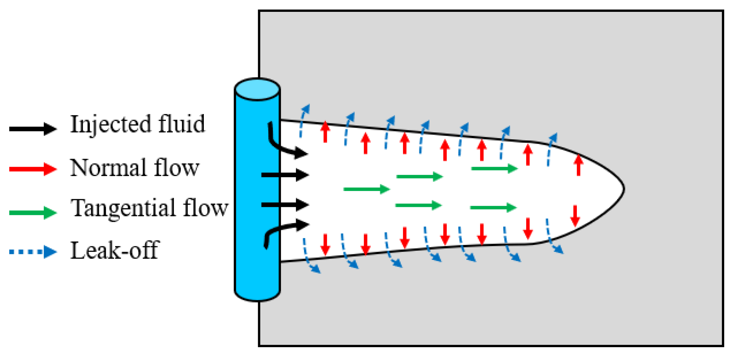
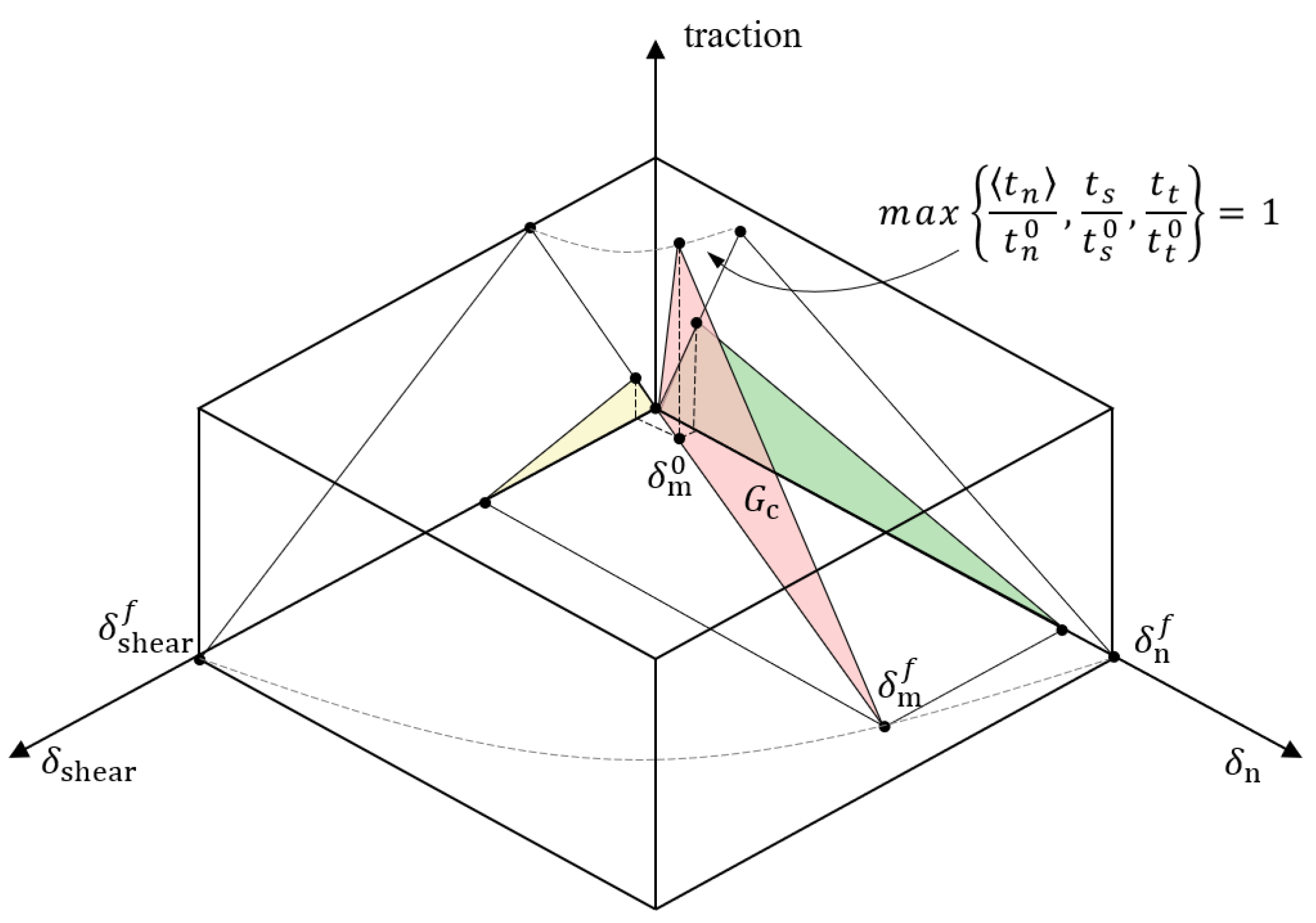
3.1. Modeling Methods for Hydraulic Fracturing

It is assumed that the fluid flowing in fractures is incompressible. The flow is then split into tangential flow, which occurs along the fracture plane, and normal flow, which occurs perpendicular to the fracture plane, as shown in Figure 7. The tangential flow rate formula for the fractures can be expressed as [55]:

$$q_i=-{\displaystyle \frac{d^3}{12\mu }}\nabla p$$

(3)

where $q_i$ is the flow velocity, $d$ is the fracture width; $p$ is the fluid pressure in the fracture, and $\mu$ is the fluid viscosity.

The flow pattern on both the upper and lower surfaces of the fracture can be described as follows [56]:

$$\left\{\begin{array}{c}{q}_t=c_t\left(p-p_t\right)\\ q_b=c_b\left(p-p_b\right)\end{array}\right\}$$

(4)

where $q_t$ and $q_b$ are the volume flow rates of the upper and lower surfaces of the fracture, respectively; $c_t$ and $c_b$ represent the filtration coefficient; $p_t$ and $p_b$ are the pore fluid pressures on both the top and bottom sides of the breakage, respectively.

Hydraulic fracturing simulation is depicted as shown in Figure 7. Fracturing fluid is injected into the fracture through the wellbore, and under the effect of fluid pressure, the crack is opened. When the fluid pressure at the tip reaches the strength of the formation, the crack will propagate and begin to extend.

In hydraulic fracturing simulation calculation, the element damage mode of the CZM follows the traction-separation law, and in its core lies the relationship between the traction force and separation displacement. The process of rock damage and hydraulic fracture propagation is governed by the traction-separation law. The traction force acting on a cohesive element can be expressed as:

$$\left\{\begin{array}{c}{t}_n\\ t_s\\ t_t\end{array}\right\}=\left[\begin{array}{ccc}{E}_{nn}& E_{ns}& E_{nt}\\ E_{sn}& E_{ss}& E_{st}\\ E_{tn}& E_{ts}& E_{tt}\end{array}\right]\left\{\begin{array}{c}{\delta }_n/T_0\\ {\delta }_s/T_0\\ {\delta }_t/T_0\end{array}\right\}$$

(5)

where $t_n$ is the normal stress exerted on the element, $t_s$ and $t_t$ are the shear stresses exerted on the element in two directions, $E_{nn}$, $E_{ns}$, $E_{nt}$, $E_{ss}$, $E_{st}$, and $E_{tt}$ are the six components of the stiffness matrix of the cohesive elements, ${\delta }_n$, ${\delta }_s$, and ${\delta }_t$ are the normal and shear separation. $T_0$ is the thickness of the initial cohesive element.

In numerical simulations, the bedding plane is selected as the x-y plane, with the outward normal direction of the bedding plane parallel to the z-axis. According to this treatment, $E_{ns}=E_{nt}=E_{sn}=E_{st}=E_{tn}=E_{ts}=0$. The other components of the stiffness matrix $E_{nn}$, $E_{ss}$, and $E_{tt}$ could be obtained from the tensile moduli for the vertical bedding planes and parallel bedding planes as per Table 4 and Table 5, respectively. $T_0$ is the thickness of the initial cohesive element.

As shown in Figure 8, the total fracture energy is represented by the area of the pink triangle, which can be divided into a yellow part (the shear component) and a green part (the normal component). When the fracture energy reaches the critical energy, the material will be completely failed and unable to support any traction force. As the initial damage criterion, a quadratic nominal stress criterion is widely used in hydraulic fracturing simulations [57]. As shown in Figure 8, $t_n^0$ is the critical normal stress for the failure of the element; $t_s^0$ and $t_t^0$ are the critical tangential stresses of failure in the two directions of the element. The symbol <> signifies that the element can withstand tensile stress and does not undergo damage when subjected to compressive stress. Once the damage criterion is reached, the traction force decreases with the increase in the separation displacement according to:

$$\begin{array}{c}{t}_n=\left\{\begin{array}{c}\left(1-D\right){\stackrel{\_}{t}}_n\\ {\stackrel{\_}{t}}_n\end{array}\right.\begin{array}{c}\left({\stackrel{\_}{t}}_n\ge 0\right)\\ otherwise\end{array}\\ t_s=\left(1-D\right){\stackrel{\_}{t}}_s\\ t_t=\left(1-D\right){\stackrel{\_}{t}}_t\end{array}$$

(6)

where ${\stackrel{\_}{t}}_n$ and ${\stackrel{\_}{t}}_s$ are the stress components expressed in Equation (5), determined by the elastic traction-separation behavior for the current strains without any damage. D is the damage factor. A material with a D value of 0 would not have yet experienced any damage. Conversely, a material with a D value of 1 would have undergone complete damage. The calculation formula for the damage factor D is as follows:

$$D={\displaystyle \frac{{\delta }_m^f\left({\delta }_m^{max}-{\delta }_m^0\right)}{{\delta }_m^{max}\left({\delta }_m^f-{\delta }_m^0\right)}}$$

(7)

where ${\delta }_m^{max}$ is the maximum displacement achieved by the element in the loading process; ${\delta }_m^f$ is the displacement when the element is destroyed, and ${\delta }_m^0$ is the displacement of the element at damage initiation.

After the initiation, fracture propagation is followed by the Benzeggagh–Kenane criterion that is described by:

$$G_{\mathrm{IC} }+\left(G_{\mathrm{IIC} }-G_{\mathrm{IC} }\right)\left({\displaystyle \frac{G_{\mathrm{II} }}{G_{\mathrm{I}}+G_{\mathrm{II} }}}\right)=G_{\mathrm{C}}$$

(8)

where $G_{\mathrm{I}}$ and $G_{\mathrm{II}}$ are the fracture energy in the normal mode and shear mode, respectively, and the subscript $C$ indicates the critical value of the fracture energy.

3.2. Multi-Cluster Hydraulic Fracturing in Shale Reservoirs with Natural Fractures

During the process of multi-cluster fracturing, the hydraulic fractures may intersect each other while propagating, which can significantly influence the trends in the fracture propagation and initiation pressure [21]. The objective of this study was to investigate the perforation fracturing process in shale horizontal wells with multiple clusters of natural fractures. A three-dimensional finite element model has been established for a subsurface setting approximately 1305 m deep, incorporating three horizontal wells and one natural fracture. As shown in Figure 9 below, the specific model had dimensions of 20 m × 20 m × 10 m and exhibited natural fracturing with a horizontal tilt angle of 15° and a length of 18 m (red area in Figure 3). Injection wells (Wells 1, 2, and 3) and natural fractures were preset. The spacing of two adjacent injection wells was 5 m, the water injection well was located at the central position of the model, and the three wells were injected simultaneously. The model was meshed using 16,710 elements, and COH3D8P elements (the COH3D8P element is a 12-node three-dimensional cohesive element) were set to simulate the 3D nonlinear fracture propagation on the planes vertical to the direction of the lowest horizontal ground stress of the reservoir.

Based on the mechanical parameters of the shale, such as elastic compression modulus, Poisson’s ratio, compressive strength, tensile strength, and tensile modulus, obtained in Table 2, Table 3, Table 4 and Table 5 and actual engineering test data [24,30],

Table 6. Parameters of multi-cluster hydraulic fracturing of shale reservoirs with natural fractures (Case 1).

Parameter	Parallel to the Bedding	Vertical to the Bedding	Parameter	Value
$\mathrm{Compression} \mathrm{modulus} E_c$ (GPa)	28.13	28.57	$\mathrm{Reservoir} \mathrm{vertical} \mathrm{ground} \mathrm{stress} {\sigma }_v$ (MPa)	32
$\mathrm{Tensile} \mathrm{modulus} E_t$ (GPa)	4.81	3.64	$\mathrm{Maximum} \mathrm{horizontal} \mathrm{ground} \mathrm{stress} \mathrm{of} \mathrm{reservoir} {\sigma }_h^{max}$ (MPa)	30
$\mathrm{Poisson}’\mathrm{s} \mathrm{ratio} \nu$	0.13	0.15	$\mathrm{Minimum} \mathrm{horizontal} \mathrm{ground} \mathrm{stress} \mathrm{of} \mathrm{reservoir} {\sigma }_h^{min}$ (MPa)	28
$\mathrm{Compressive} \mathrm{strength} {\sigma }_{bc}$ (MPa)	191.08	123	$\mathrm{Reservoir} \mathrm{filtration} \mathrm{coefficient} c_1$ (m/s1/2)	1 × 10−14
Shear stiffness (GPa/m)	3000	3000	$\mathrm{Natural} \mathrm{fracture} \mathrm{filtration} \mathrm{coefficient} c_2$ (m/s1/2)	1 × 10−13
$\mathrm{Tensile} \mathrm{strength} {\sigma }_t$ (MPa)	6.04	13.98	$\mathrm{Natural} \mathrm{fracture} \mathrm{tensile} \mathrm{strength} {{\sigma }_t}^{\prime }$ (MPa)	2
$\mathrm{Hydraulic} \mathrm{fracture} \mathrm{energy} G_c$ (Pa·m)	5000	5000	$\mathrm{Natural} \mathrm{fracture} \mathrm{energy} {G_c}^{\prime }$ (Pa·m)	1000
$\mathrm{Density} \rho$ (g/cm3)	2.5	2.5	$\mathrm{Injection} \mathrm{rate} Q$ (L/min)	60
Initial porosity e (%)	3	3	Fluid viscosity $\eta$ (mPa·s)	1

presents the hydraulic fracturing simulation parameters for multi-cluster hydraulic fractures in the shale reservoirs with natural fractures. To investigate the effects of the variables associated with hydraulic fracturing, the case in Table 6 is called Case 1. Here, the vertical ground stress of the reservoir was 32 MPa, the maximum horizontal ground stress of the reservoir was 30 MPa, and the lowest ground stress in the horizontal direction of the reservoir was 28 MPa. In Case1, each well has an injection rate of 60 L/min, with all three wells injecting simultaneously. The other cases are listed in

Table 7. Material parameters of the other four cases.

Case	${\mathit{\sigma }}_{\mathit{v}}$ (MPa)	${\mathit{\sigma }}_{\mathit{h}}^{\mathit{m}\mathit{a}\mathit{x}}$ (MPa)	${\mathit{\sigma }}_{\mathit{h}}^{\mathit{m}\mathit{i}\mathit{n}}$ (MPa)	$\mathit{Q}$ (L/min)	$\mathit{\eta }$ (m·Pa)
Case 2	34 MPa	30 MPa	28 MPa	60 L/min	1 mPa·s
Case 3	32 MPa	—	25 MPa	—	—
Case 4	—	—	28 MPa	30 L/min	—
Case 5	—	—	—	30 L/min	20 mPa·s

, which shows only the parameters that are different from Case 1.

In the fracture propagation simulation, the hydraulic fractures may interact with the natural fractures. Therefore, it is necessary to apply a special treatment to the CZM elements to ensure the continuity of the fluid flow at the intersections of 3D fractures. Figure 10a shows the grid diagram at the intersection of these fractures; Figure 10b shows the arrangement diagram of the pore pressure nodes at the intersection between the 3D hydraulic fractures and natural fractures. Notably, each fracture element comprises nodes representing the pore pressure, indicated by the blue dots in Figure 10b. To achieve continuity, the pore pressure nodes located at the intersection of the fractures are combined, as depicted in Figure 10c. Specifically, the pore pressure node 1 of the natural fracture element is merged with the pore pressure node 3 of the adjacent natural hydraulic element. Similarly, the pore pressure node 2 of the natural fracture element is combined with the pore pressure node 4 of the adjacent hydraulic fracture element. By combining the pore pressure nodes at the intersection of the fractures, the pressure is transferred within the fluid. Consequently, the flow continuity at the fracture intersection is ensured. This enables the simulation of the propagation of 3D fractures at the intersection points.

4. Results and Analysis

In this section, first, the results of Case 1 (the parameters of which are shown in Table 6) are presented. The effects of the ground stress and fracturing conditions (the parameters of which are shown in Table 7) on fracture propagation are then discussed.

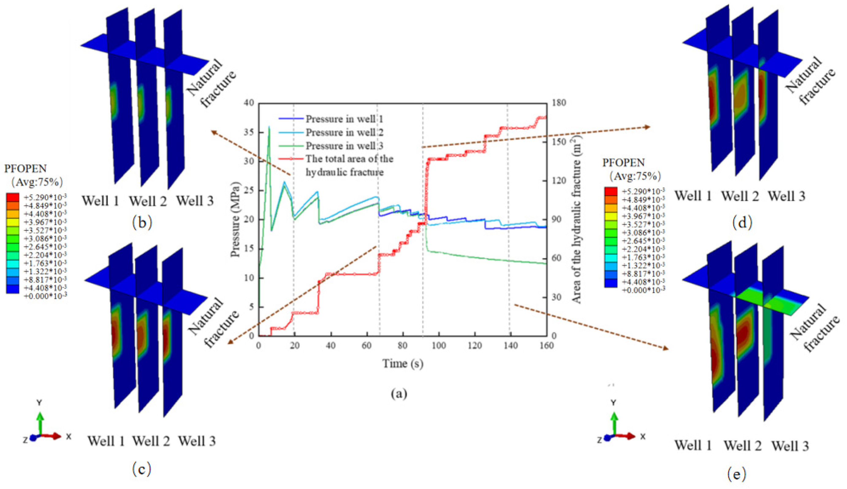
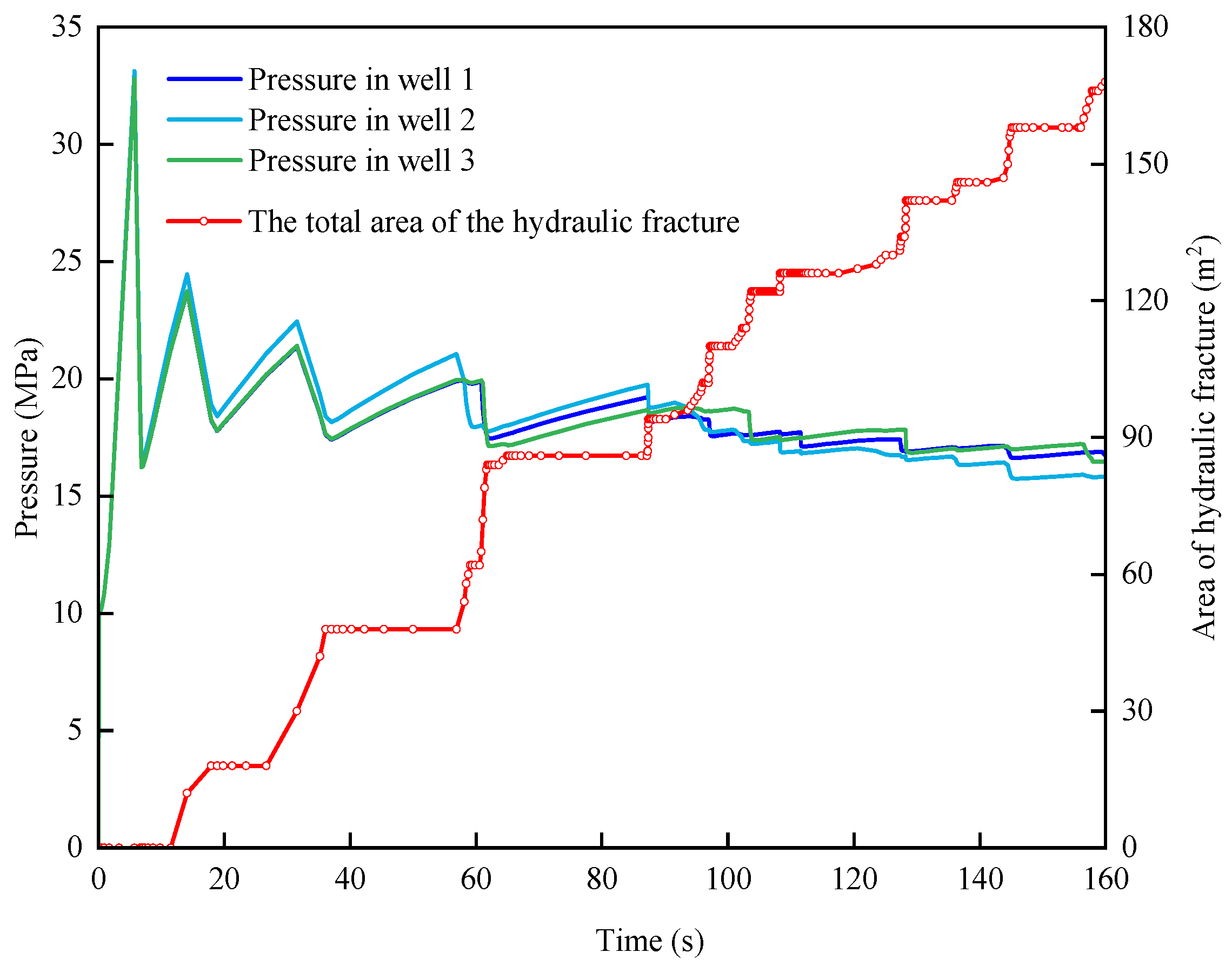
4.1. Hydraulic Fracture Propagation in Case 1

Figure 11 shows the bottom-hole pressure, hydraulic fracture area, and fracture shape at the corresponding time for Case 1. As shown in Figure 11a, the bottom-hole pressures in Wells 1, 2, and 3 do not differ significantly during the initial injection phase. The bottom-hole pressure increases from 12 MPa to 31 MPa and then drops rapidly to 18 MPa. With the decrease in the bottom-hole pressure, the hydraulic fractures enlarge. During this stage, the hydraulic fractures gradually expand, and the PFOPEN (the opening displacements of a crack) in Figure 11b (t = 20 s) shows that the fracture shape is semi-circular. In Figure 11c (t = 75 s), the three hydraulic fractures continue to expand and interfere with each other. The hydraulic fracture in Well 3 that extended further upward near the natural fracture in Well 2 expanded vertically along the Z axis, which represents the maximum horizontal ground stress, while the fracture in Well 1 expanded horizontally along the Y direction.

When the injection time reaches t = 90 s, the total area of the hydraulic fractures quickly increases, and the bottom-hole pressures of Wells 1 and 2 remain the same, while the bottom-hole pressure of Well 3 drops to 17 MPa, as shown in Figure 11a. From Figure 11d, an interaction between the hydraulic fracture from Well 3 and the pre-existing natural fracture can be observed. As the injection time reaches t = 140 s, the hydraulic fractures continue to spread along the natural fractures, as depicted in Figure 11e.

The hydraulic fractures in Well 2 extended in the direction of the highest horizontal ground stress, and the hydraulic fractures in Well 1 expanded vertically in the negative direction of the Y-axis. The pressure curve and hydraulic fracture morphology obtained from the numerical calculation were in agreement with the experimental results [17].

During the actual process of hydraulic fracturing, it is crucial to highlight the significance regarding the fact that the bottom-hole pressure could be relatively stable after fracture expansion, rather than constantly fluctuating, as shown in Figure 11a. The hydraulic fracture area should also increase linearly rather than in a stepwise manner. This is because the expansion of the hydraulic fractures by the CZM depends on whether the next cohesive element is damaged, and the damaged cohesive elements are opened stepwise.

Figure 12 shows the curve of the hydraulic fracture volume with time during injection. Evidently, the hydraulic fracture volume increases suddenly after the natural fracture opens at around 9 s. This is because the filtration coefficient of the natural fractures is greater than that of the shale reservoir matrix. While the injection rate remains constant, the filtration hydraulic volume undergoes a more rapid propagation, thereby decreasing the volume expansion of the hydraulic fractures. In summary, the graph furnishes valuable insights into the dynamic nature of hydraulic fracturing processes and underscores the necessity of accurately modeling and understanding both artificial and natural fractures. This is essential for optimizing well performance and maximizing hydrocarbon recovery rates.

Figure 11 shows that the hydraulic fracture through Well 3 expands the fastest, gradually approaches the natural fracture, and then expands along the natural fracture. Due to the effect of hydraulic fracture interference, the hydraulic fracture in Well 2 expands toward the horizontal direction of the minimum ground stress, while the hydraulic fracture in Well 1 extends downward. At the beginning, the bottom-hole pressure curve of Well 2 is higher compared with those of Wells 1 and 3. However, thereafter, the bottom-hole pressure curve of Well 3 reaches its minimum point.

4.2. Influence of Ground Stress on Fracture Propagation

The ground stress in a shale gas reservoir can affect the propagation of hydraulic fractures [40]. In the following, the effects of ground stress on fracture propagation in the reservoir through Cases 2 and 3 are studied.

4.2.1. Effect of Vertical Ground Stress

To study the effect of vertical ground stress on fracture propagation, the vertical ground stress was varied from 32 MPa in Case 1 to 34 MPa for Case 2, while the other parameters were kept unchanged.

Figure 13 shows the bottom-hole pressure and hydraulic fracture area at a corresponding time during injection for Case 2. In terms of the bottom-hole pressure, the curve of Well 2 initially maintains a higher level than those of Wells 1 and 3. However, in the later stages, the bottom-hole pressure curve of Well 2 becomes lower compared with those of Wells 1 and 3. Moreover, the well-bottom pressure curves of Wells 1 and 3 have similarities. There exists an evident difference in the area of the hydraulic fractures compared with that in Case 1. From the figure, it can be observed that the increase in hydraulic fracture area might influence the pressure distribution among the wells. A larger fracture area could result in more fluids entering the fracture system, thus reducing the bottomhole pressure. The growth of the hydraulic fracture area is not linear but rather exhibits nonlinear behavior, reflecting the complexity of the fracture extension process, such as closure, reopening, or other intricate geological effects. By analyzing these data, injection strategies can be optimized to maximize hydraulic fracture extension and enhance production efficiency. For instance, adjusting the injection rate or pressure can control the fracture’s expansion to achieve the most favorable fracture geometry and maximum fracture area.

Figure 14 shows the hydraulic fracture shape in Case 2 when the injection times are t = 109 s and t = 140 s. In Figure 14a, the hydraulic fracture in Well 2 interacts with the natural fracture at t = 109 s and expands upward, while the hydraulic fractures in Wells 1 and 3 expand in a downward direction due to the interference from hydraulic fractures. The hydraulic fracture in Well 2, shown in Figure 14b, continues to expand within the existing natural fracture, and the natural fracture remains unopened. Figure 14 shows that the fracture shape in Case 2 is significantly different from that in Case 1, in which the hydraulic fracture induced by Well 3 interacts with the natural fracture, and the natural fracture is opened.

Figure 15 shows the volume of the hydraulic fracture during injection under different vertical ground stress conditions in Cases 1 and Case 2; Figure 16 shows the filtration loss over time in the two cases. During the initial injection stage, the varying vertical ground stress does not significantly affect the volume of the hydraulic fracture and the extent of filtration loss. However, during the later stages of injection, the volume growth of the hydraulic fractures decelerates after the opening of the natural fracture in Case 1, whereas in Case 2, a strong linear correlation can be seen with the injection time. This phenomenon can be attributed to the fact that the filtration coefficient of the natural fracture exceeds that of the shale reservoir matrix. After the opening of the natural fracture in Case 1, as time progresses, the filtration loss in Case 1 becomes increasingly greater than that in Case 2, as shown in Figure 16.

Notably, in Figure 15, the volume of hydraulic fractures is measured based on the cumulative volume from three wells. Assuming each well has an injection rate of 60 L/min (equivalent to 0.06 m³), the combined injection rate for all three wells would be 0.18 m³. According to this rate, the theoretical volume of fluid injected after 60 s would be 0.18 m³. However, Figure 11 illustrates that at the 60 s mark, the observed fracture volume is approximately 0.12 m³. This discrepancy can be attributed to partial fluid loss, estimated at around 0.06 m³ at the 60 s interval. Therefore, taking into account the effect of fluid loss, the actual volume within the fractures is less than the theoretical value.

The following observations can be made from the changes in the fracture growth morphology and fracture volume with time under different vertical ground stresses in Cases 1 and 2: When the vertical ground stress is low, as in Case 1, in the initial phase, the natural fractures significantly influence the expansion of the hydraulic fractures. The hydraulic fracture closest to the natural fracture experiences a faster expansion, gradually approaching the natural fracture, and the natural fracture is opened after intersecting with the natural fracture. When the vertical ground stress of the reservoir is high, as in Case 2, the main factor controlling the hydraulic fracture propagation is the vertical ground stress of the reservoir. The hydraulic fracture of the injection well located in the middle expands at a higher rate, gradually reaching the natural fracture and eventually passing through it once they have merged.

4.2.2. Effect of the Difference in the Horizontal Ground Stress

To study the effect of the horizontal ground stress on fracture propagation, the difference in the horizontal ground stress was varied from 2 MPa in Case 1 to 5 MPa in Case 3, while the other parameters were kept unchanged.

Figure 17 shows the fracture shape in Case 3, in which the horizontal ground stress difference is 5 MPa when t = 111 s and t = 140 s. In this case, the hydraulic fracture in Well 3 interacts with the natural fracture at t = 111 s and expands upward by passing through the natural fracture after encountering it, rather than propagating along the natural fracture as in Case 1. The hydraulic fracture in Well 2 propagates downward due to fracture interference. Fracture interference causes the expansion of fractures in Well 1 toward the direction of the maximum horizontal ground stress.

Figure 18 shows the pressure at the bottom hole of Well 3 and the hydraulic fracture area of all the wells in Case 3. Compared with Case 1, the area of the fracture observed in Case 3 continues to steadily increase around t = 90 s, whereas it rapidly increases at this time in Case 1. The pressure change in Well 3 in Case 3 is not significant compared with that in Case 1 at t = 90 s. This is because the natural fracture has not been clearly opened. This phenomenon is in accordance with the fracture shape shown in Figure 18.

When the difference in the horizontal ground stress changes from 2 MPa to 5 MPa, the fracture propagation is dominated by the vertical ground stress of the reservoir, and after the hydraulic fractures intersect with the natural fractures, they expand upward and cross through the natural fractures. Simultaneously, the hydraulic fractures in the adjacent intermediate injection wells spread downward due to the fracture interference.

4.3. Effect of Injection Conditions on Fracture Propagation

The injection parameters influence the propagation of hydraulic fractures. The effects of injection parameters on the reservoir fracture growth were studied through Cases 4 and 5.

4.3.1. Effect of Injection Rate

To study the effect of the injection rate on fracture growth, the injection rate in Case 1 was varied from 60 L/min to 30 L/min in Case 4, while the other parameters were kept unchanged.

Figure 19 shows the fracture shape in Case 4, in which the injection rate is 30 L/min when t = 265 s and t = 270 s. In this case, the hydraulic fracture of Well 3 interacts with the natural fracture at t = 265 s, and then 5 s later, it propagates along the natural fracture. Compared with Case 1, the time required for the hydraulic fracture induced by Well 3 to intersect the natural fracture changes from 90 s in Case 1 to 265 s in Case 4.

Figure 20 shows the bottom-hole pressure over time at different injection rates. Evidently, when the injection rate is 30 L/min in Case 4, the initial bottom-hole pressure is lower compared with that in Case 1. The time required for convergence between the hydraulic and natural hydraulic fractures in Case 4 increases, and more time is required for the sharp drop in the bottom-hole pressure of Well 2. The lowest bottom-hole pressure at an injection rate of 30 L/min in Case 4 does not differ significantly from that observed at an injection rate of 60 L/min in Case 1.

Figure 21 shows the hydraulic fracture area with time under different injection rates. A variation in the injection rate of the fracturing fluid brings about a corresponding change in the hydraulic fracture area over time.

By analyzing the changes in the pressure at the bottom of the hole and the hydraulic fracture area over time at different injection rates, it becomes evident that a higher injection rate corresponds to increased pressure at the bottom hole during the pressure-holding stage, accelerated growth of the hydraulic fracture area, and faster fracture expansion.

4.3.2. Effect of Fracturing Fluid Viscosity

To study the effect of the fracturing fluid viscosity on the fracture growth, the injection fluid viscosity in Case 4 was varied from 1 mPa·s to 20 mPa·s in Case 5, while the other parameters were kept unchanged.

Figure 22 shows the fracture shape in Case 5, in which the injection rate is 30 L/min and the injection fluid viscosity is 20 mPa·s when t = 200 s and t = 270 s. In this case, the hydraulic fracture in Well 3 interacts with the natural fracture when t = 200 s. From Figure 22b, the propagation of the hydraulic fracture induced by Well 3 along the natural fractures is evident. The time required for the hydraulic fracture induced by Well 3 to intersect the natural fracture in Case 5 is 200 s, which is longer than that (90 s) in Case 1 and shorter than that (265 s) in Case 4. Compared with Figure 19b, from Figure 22b, it is evident that with the increase in the injection fluid viscosity, the opened area of the natural fracture is greater than that in Case 4.

Figure 23 shows the temporal variation in the bottom-hole pressure. Notably, once the viscosity of the fracturing fluid reaches 20 mPa·s, the convergence of the hydraulic and natural fractures becomes more rapid compared with that in Case 4. Consequently, the time taken for the bottom-hole pressure of Well 3 to sharply decrease is shorter. Figure 24 shows the temporal variation in the hydraulic fracture area under different fracturing fluid viscosities. When the viscosity of the injection fluid is 20 mPa·s, the area propagation rate is greater than that when the viscosity is 1 mPa·s. By comparing the temporal variation in the pressure at the bottom hole and hydraulic fracture area under different fracturing fluid viscosities, it can be found that when the viscosity of the fracturing fluid increases, the hydraulic fracture intersects with the natural fracture more quickly, leading to a more rapid fracture expansion. Consequently, a higher fracturing fluid viscosity results in an accelerated propagation of the hydraulic fractures.

5. Conclusions

This chapter involves cutting and processing the outcrop shale from the Changning area in Yibin City, Sichuan Province, to prepare core samples parallel and vertical to the bedding planes. Uniaxial compression tests and Brazilian splitting tests were conducted to obtain the mechanical parameters of shale compression and tension. The anisotropic mechanical parameters of shale were systematically characterized in both bedding-perpendicular and bedding-parallel orientations. The elastic compressive modulus, Poisson’s ratio, compressive strength, tensile modulus, and tensile strength of the shale with parallel and vertical bedding planes were calculated and compared. Experimental results demonstrated significant anisotropic behavior in the studied shale formations. The quantified anisotropy parameters were subsequently implemented in a finite element model for hydraulic fracturing simulation. A 3D multi-cluster fracturing model of a heterogeneous shale reservoir with natural fractures was established, and the complex 3D fracture morphologies after the interaction between any two fractures were revealed. The bottom-hole pressure, hydraulic fracture area volume, and hydraulic fracture propagation morphology at the corresponding time under different reservoir conditions were obtained. The effects of the reservoir conditions and fracture propagation conditions were studied and discussed. This computational framework enabled comprehensive investigation of fracture propagation patterns and three-dimensional morphology evolution under anisotropic geomechanical conditions, providing critical insights into hydraulic fracture-geological structure interactions in shale reservoirs. The results are summarized as follows:

(1)

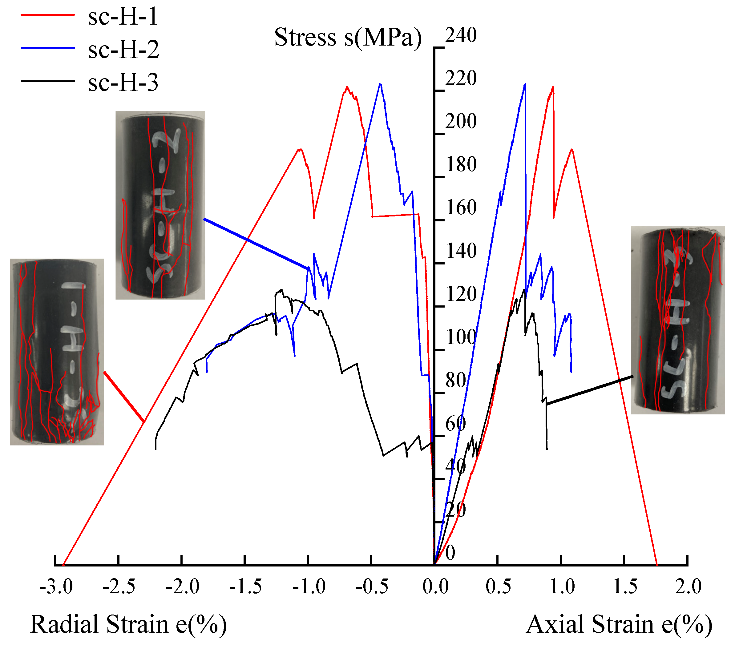
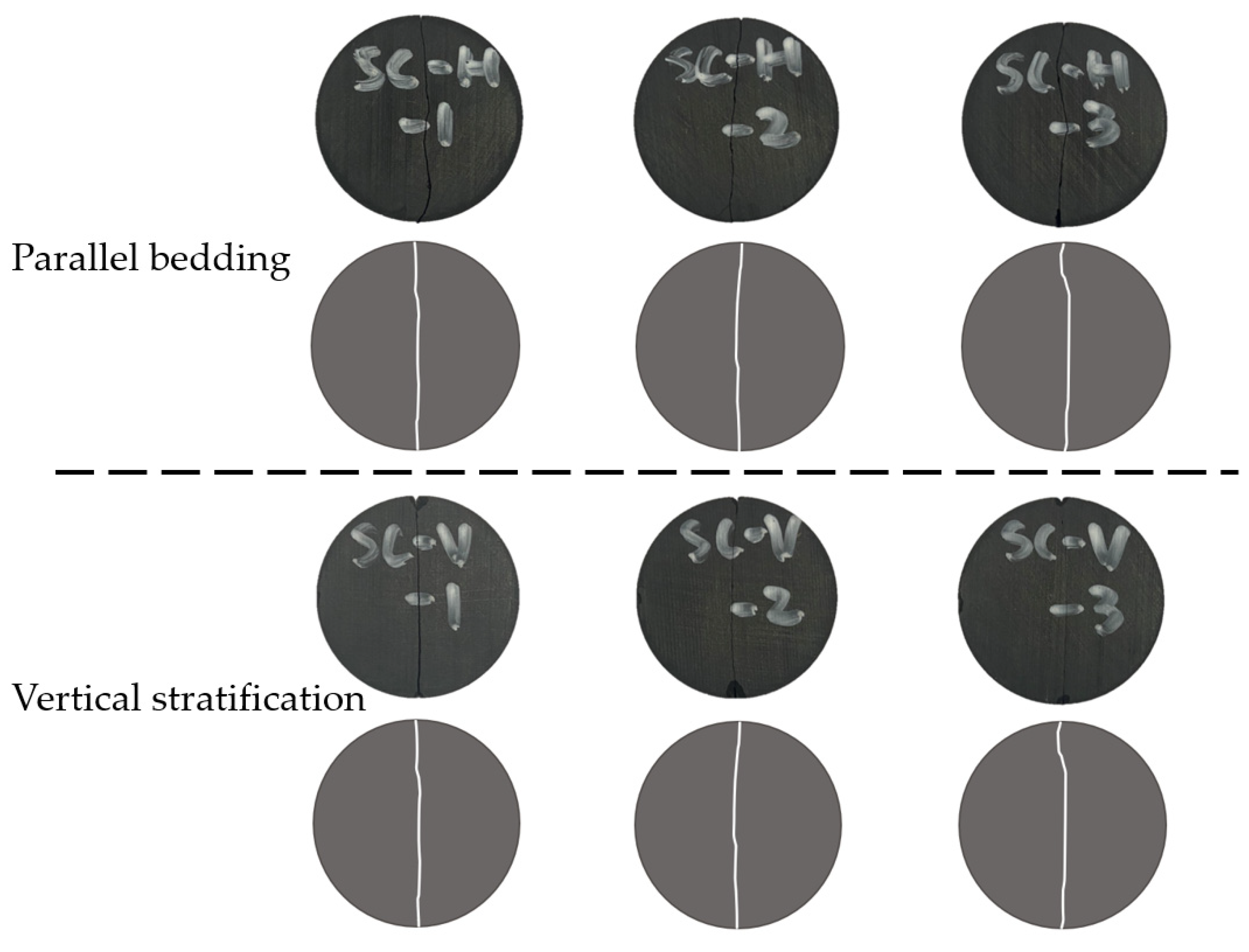
The shale samples exhibit distinct bedding planes, showing significant anisotropy. The elastic compressive modulus and Poisson’s ratio of the parallel bedding shale samples are similar to those of the vertical bedding shale samples, while the compressive strength of the parallel bedding shale samples is significantly greater than that of the vertical bedding shale samples. The elastic compressive modulus of the parallel bedding shale samples ranges from 22.42 to 32.74 GPa with a Poisson’s ratio between 0.11 and 0.15 and a compressive strength ranging from 127.82 to 223.21 MPa. The elastic compressive modulus of the vertical bedding shale samples ranges from 25.56 to 31.90 GPa with a Poisson’s ratio between 0.13 and 0.18 and a compressive strength ranging from 83.53 to 158.22 MPa.

(2)

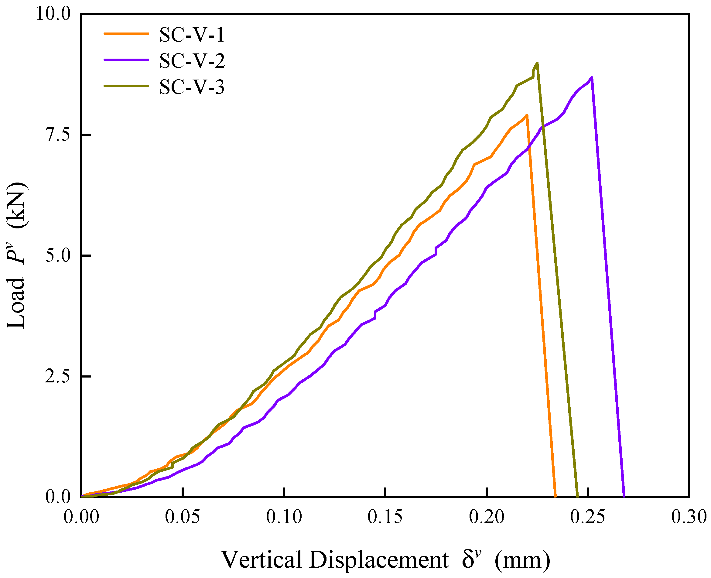
The anisotropy in the tensile performance of shale by Brazilian splitting test is significant. Both vertical and horizontal bedding shale curves from the tests show increasing load with more vertical displacement, then a sharp drop in load. The ultimate failure load and tensile strength of the parallel bedding shale samples are less than those of the vertical bedding shale samples. The ultimate failure load of the parallel bedding shale samples ranges from 2.20 to 4.51 kN with a tensile strength of 3.68 to 7.54 MPa. The ultimate failure load of the vertical bedding shale samples ranges from 7.91 to 8.98 kN with a tensile strength of 13.01 to 14.65 MPa.

(3)

The tensile modulus of the parallel bedding shale samples is greater than that of the vertical bedding shale samples. The tensile modulus of the parallel bedding shale samples ranges from 4.52 to 5.19 GPa, while the tensile modulus of the vertical bedding shale samples ranges from 3.52 to 3.75 GPa. The elastic compressive modulus of the shale is 6 to 10 times the tensile modulus.

(4)

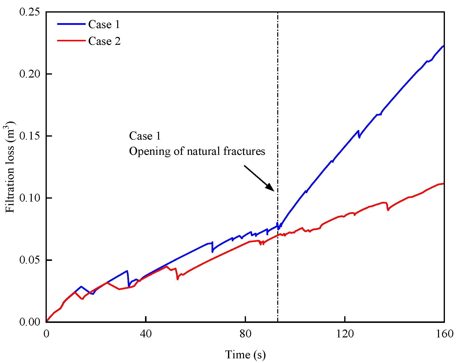
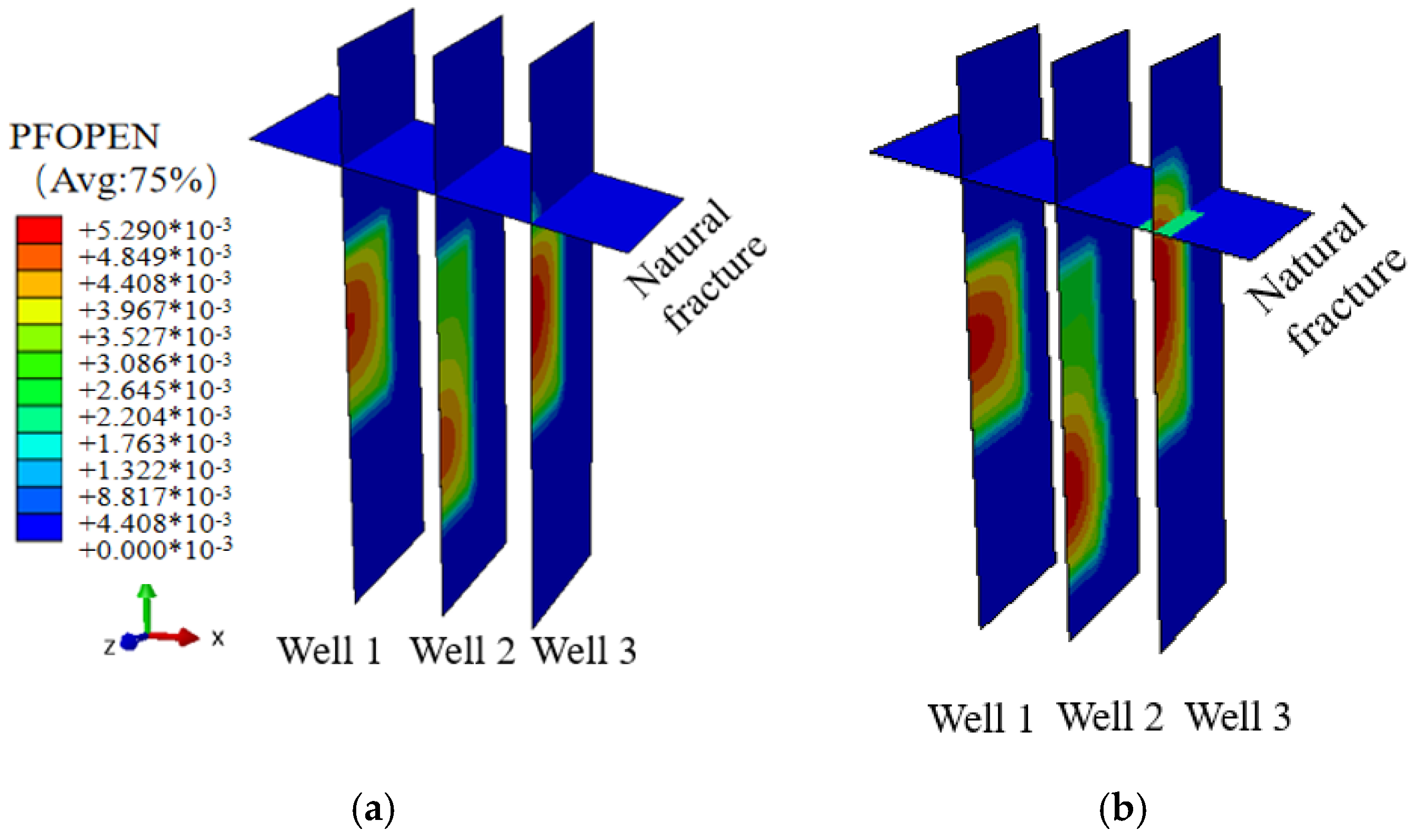
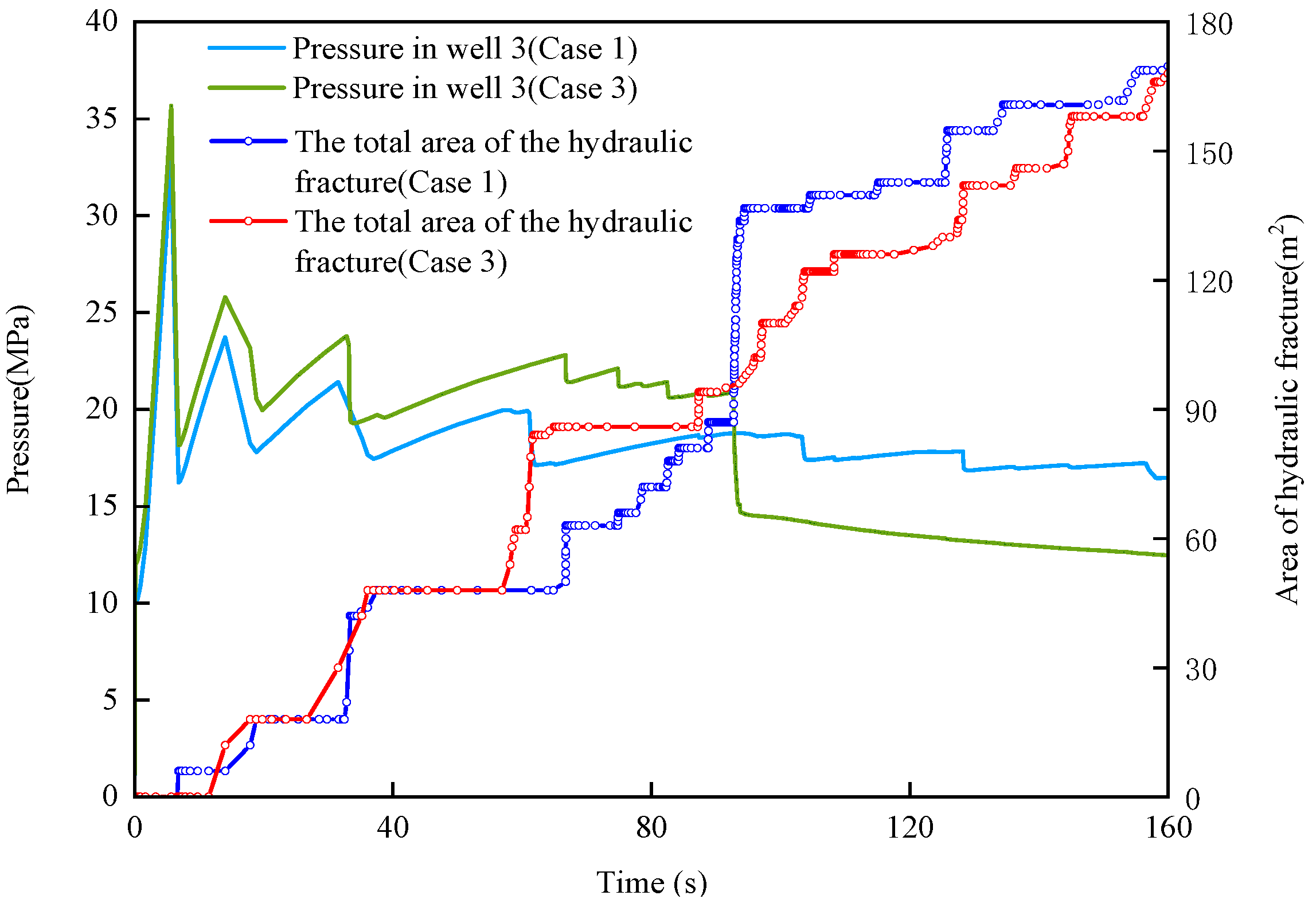
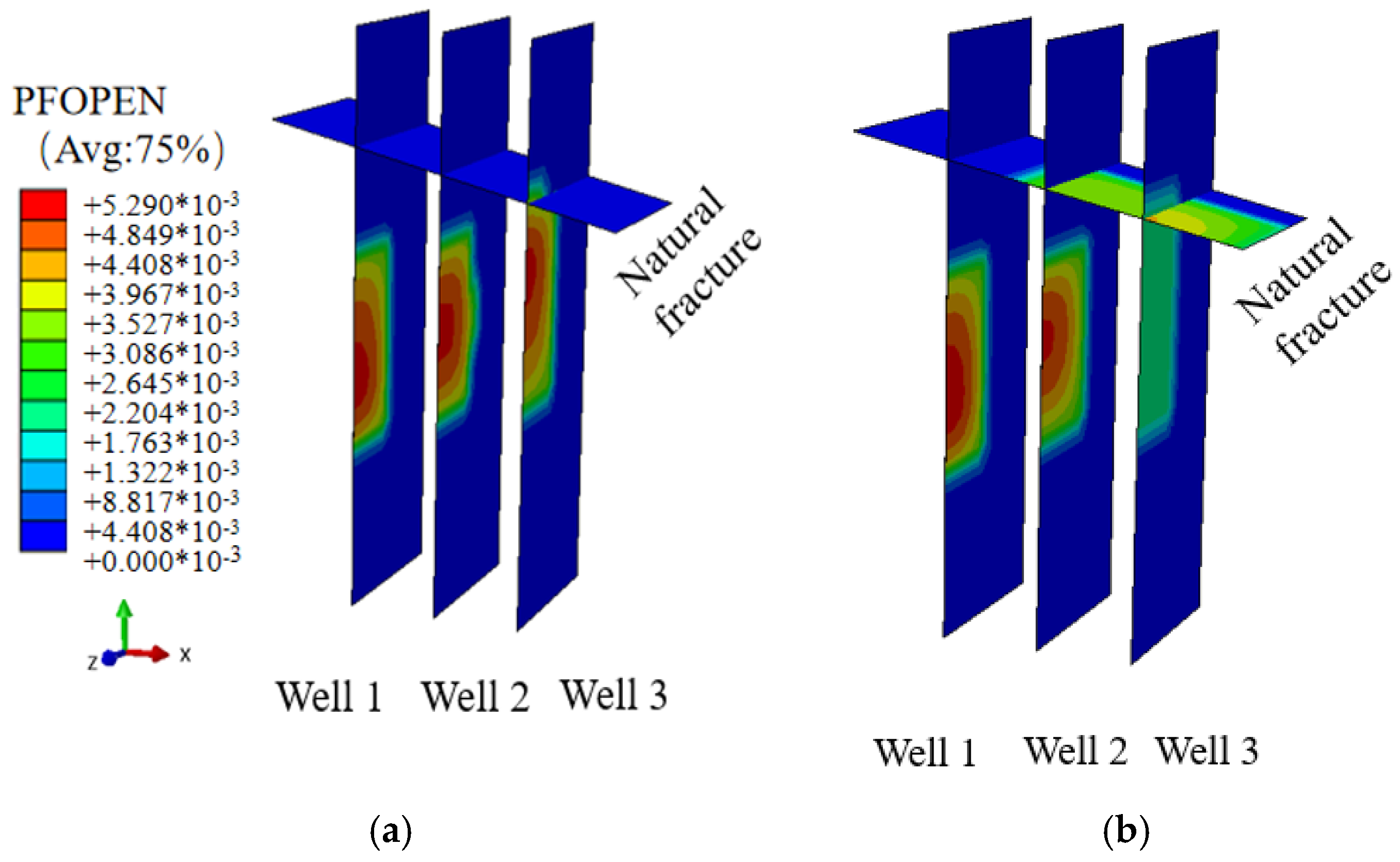
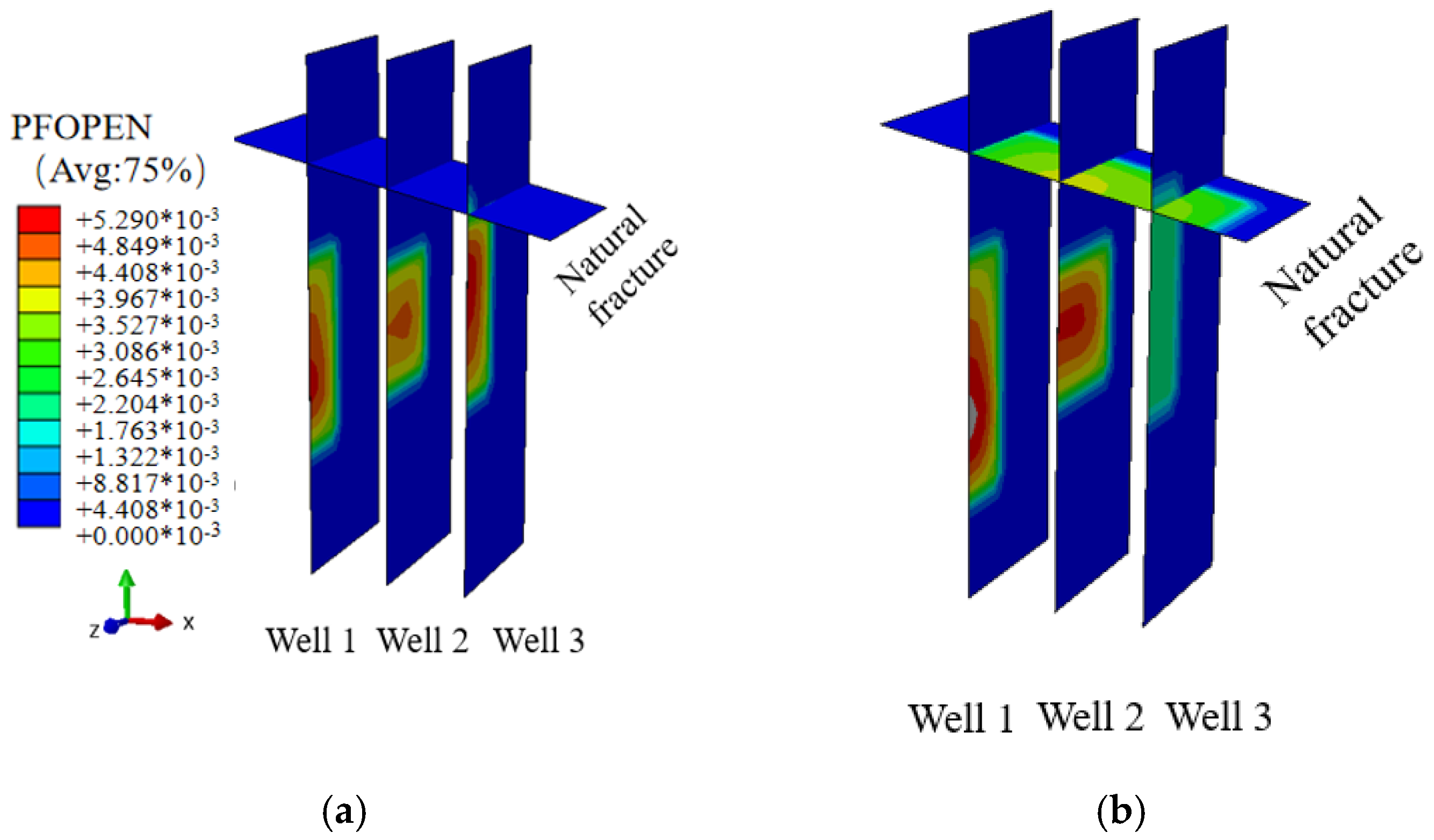
Under two different levels of the vertical ground stress (Cases 1 and 2), when the vertical ground stress of the reservoir was low, the hydraulic fracture induced by the injection well closest to the natural fracture expanded the fastest, and the natural fracture opened when it intersected with the hydraulic fracture. Through studies on two different levels of the horizontal ground stress (Cases 1 and 3), it was evident that when there was a greater difference in the horizontal ground stress, the natural fractures were more inclined to open after the point at which the hydraulic and natural fractures intersected.

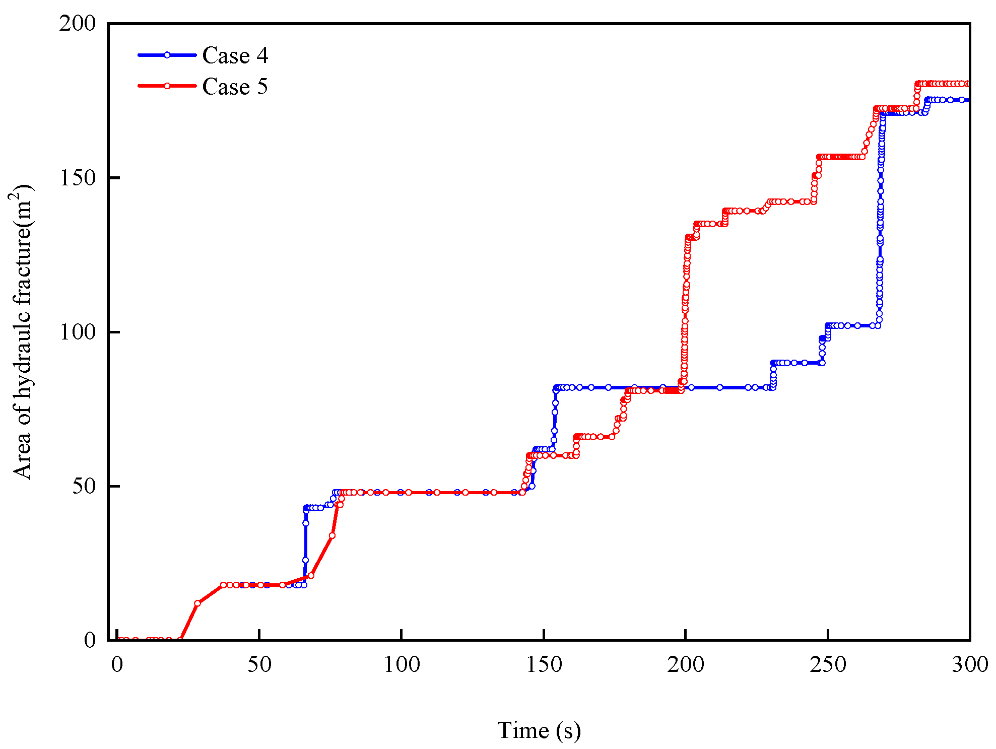
(5)

The results from Case 4 revealed that as the injection rate increased, there was a corresponding increase in the initial pressure, the speed at which the hydraulic fracture area increased, and the speed of fracture spreading. Compared with the simulation results from Cases 4 and 5, it was evident that a higher viscosity of the fracturing fluid led to a faster propagation of the hydraulic fractures.

(6)

The experimental and numerical research findings could improve the fracturing process through a better understanding of the fracture propagation process and offer a scientific foundation for the efficient development of shale gas reservoirs and to foster advancements in hydraulic fracturing technology.

References

1. Fateh, B.; Aisha, A.; Raed, A. Balancing climate mitigation and energy security goals amid converging global energy crises: The role of green investments. Renew. Energy 2023, 205, 534–542. [Google Scholar] [CrossRef]
2. Li, S.; Hu, Z.; Chang, X. Mechanistic study on the influence of stratigraphy on the initiation and expansion pattern of hydraulic fractures in shale reservoirs. Appl. Sci. 2022, 16, 8082. [Google Scholar] [CrossRef]
3. Weber, N.; Fries, T. The XFEM with an Implicit-Explicit Crack Description for a Plane-Strain Hydraulic Fracture Problem. PAMM 2013, 1, 83–84. [Google Scholar] [CrossRef]
4. Wang, X.; Shi, F.; Liu, H.; Wu, H. Numerical simulation of hydraulic fracturing in orthotropic formation based on the extended finite element method. J. Nat. Gas Sci. Eng. 2016, 33, 56–69. [Google Scholar] [CrossRef]
5. Fatahi, H.; Hossain, M.M.; Sarmadivaleh, M. Numerical and experimental investigation of the interaction of natural and propagated hydraulic fracture. J. Nat. Gas Sci. Eng. 2017, 37, 409–424. [Google Scholar] [CrossRef]
6. Olga, K.; Weng, X. Numerical Modeling of 3D Hydraulic Fractures Interaction in Complex Naturally Fractured Formations. Rock Mech. Rock Eng. 2018, 51, 3863–3881. [Google Scholar] [CrossRef]
7. Xie, L.; Min, K.B.; Shen, B. Simulation of hydraulic fracturing and its interactions with a pre-existing fracture using displacement discontinuity method. J. Nat. Gas Sci. Eng. 2016, 36, 1284–1294. [Google Scholar] [CrossRef]
8. Shakib, T.J.; Shahri, A.G.A. Analysis of hydraulic fracturing in fractured reservoir: Interaction between hydraulic fracture and natural fractures. Life Sci. J. 2012, 9, 1862. [Google Scholar] [CrossRef]
9. Chen, M.; Li, M.; Wu, Y.; Bang, K. Simulation of hydraulic fracturing using different mesh types based on zero thickness cohesive element. Processes 2020, 82, 189. [Google Scholar] [CrossRef]
10. Hunsweck, M.; Shen, Y.; Lew, A. A finite element approach to the simulation of hydraulic fractures with lag. Int. J. Numer. Anal. Methods Geomech. 2013, 79, 993–1015. [Google Scholar] [CrossRef]
11. Zhou, J.; Zhang, L.; Braun, A.; Han, Z. Numerical Modeling and Investigation of Fluid-Driven Fracture Propagation in Reservoirs Based on a Modified Fluid-Mechanically Coupled Model in Two-Dimensional Particle Flow Code. Energies 2016, 9, 699. [Google Scholar] [CrossRef]
12. Carrier, B.; Granet, S. Numerical modeling of hydraulic fracture problem in permeable medium using cohesive zone model. Eng. Fract. Mech. 2012, 79, 312–328. [Google Scholar] [CrossRef]
13. Wang, D.; Dong, Y.; Sun, D.; Yu, B. A three-dimensional numerical study of hydraulic fracturing with degradable diverting materials via CZM-based FEM. Eng. Fract. Mech. 2020, 237, 107251. [Google Scholar] [CrossRef]
14. Ping, E.; Zhao, P.; Zhu, H.; Zi, J.; Qing, Z.; Gan, F. Numerical Simulation of the Simultaneous Development of Multiple Fractures in Horizontal Wells Based on the Extended Finite Element Method. Energies 2024, 17, 1057. [Google Scholar] [CrossRef]
15. Wen, J.; Xiang, T.; Zhu, M.; Hu, P.; Mao, J.; Jing, Y.H. Investigation of shale hydraulic fracturing propagation laws based on extended finite element analysis. Drill. Eng. 2022, 5, 177–188. [Google Scholar]
16. Cherny, S.; Lapin, V.; Esipov, D.; Avdyushenko, A.; Lyutov, A.; Karnakov, P. Simulating fully 3D non-planar evolution of hydraulic fractures. Int. J. Fract. 2016, 2, 209–211. [Google Scholar] [CrossRef]
17. Zhang, F.; Wang, X.; Tang, M.; Du, X.F.; Xu, C.C.; Tang, J.Z.; Damjanac, B. Numerical investigation on hydraulic fracturing of extremely limited entry perforating in plug-and-perforation completion of shale oil reservoir in Changqing oilfield, China. Rock Mech. Rock Eng. 2021, 54, 2925–2941. [Google Scholar] [CrossRef]
18. Kang, X.; Jiang, M.; Huan, G.; Wu, J.N.; Tang, M.; Wang, Z.Y. Application research on fracture propagation law of combined hydraulic pressure in multiple coal fractures. J. Min. Saf. Eng. 2021, 3, 602–608. [Google Scholar]
19. Wang, Y.; Liu, N.; Wang, H. Simulation investigation on spatial deflection of multiples fractures of multistage perforation clusters in hydraulic fracturing. Coal Sci. Technol. 2023, 5, 160–169. [Google Scholar]
20. Li, M.; Zhou, D.; Su, Y. Simulation of fully coupled hydro-mechanical behavior based on an analogy between hydraulic fracturing and heat conduction. Comput. Geotech. 2023, 156, 105259. [Google Scholar] [CrossRef]
21. Wang, Y.; Ju, Y.; Zhang, H.; Song, J.X.; Li, Y.; Chen, J. Adaptive finite element-discrete element analysis for the stress shadow effects and fracture interaction behaviors in three-dimensional multistage hydrofracturing considering varying perforation cluster spaces and fracturing scenarios of horizontal wells. Rock Mech. Rock Eng. 2021, 54, 1815–1839. [Google Scholar] [CrossRef]
22. Hou, Z.; Yang, C.; Guo, Y.; Zhang, B.; Wei, Y.; Heng, S.; Wang, L. Study on the anisotropic characteristics of Longmaxi Formation shale under uniaxial compression. Rock Soil Mech. 2015, 36, 2541–2550. [Google Scholar]
23. Li, Z. Study on the Anisotropic Characteristics of Rock under Uniaxial Compression. J. Railw. Sci. Eng. 2008, 3, 69–72. [Google Scholar]
24. Jia, C.; Chen, J.; Guo, Y. Research on the Mechanical Properties and Failure Modes of Laminated Shale. Rock Soil Mech. 2013, 34 (Suppl. S2), 57–61. [Google Scholar]
25. Istvan, J.A.; Evans, L.J.; Weber, J.H.; Devine, C. Rock mechanics for gas storage in bedded salt caverns. Int. J. Rock Mech. Min. Sci. 1997, 34, 142. [Google Scholar] [CrossRef]
26. McLamore, R.; Gray, E. The mechanical behavior of anisotropic sedimentary rocks. J. Eng. Industry. 1967, 89, 62–73. [Google Scholar] [CrossRef]
27. Debecker, B.; Vervoort, A. Experimental observation of fracture patterns in layered slate. Int. J. Fract. 2009, 159, 51–62. [Google Scholar] [CrossRef]
28. Liu, Y.; Fu, H.; Rao, J.; Dong, H.; Cao, Q. Research on Brazilian disc splitting tests for anisotropy of slate under influence of different bedding orientations. Chin. J. Rock Mech. Eng. 2012, 31, 785–791. [Google Scholar]
29. Zhong, S.; Zuo, S.; Luo, S. Brazilian tensile strength and tensile damage anisotropy of laminated limestone. Sci. Technol. Eng. 2020, 20, 6578–6584. [Google Scholar]
30. Guo, W.; Guo, Y.; Yang, H.; Wang, L.; Liu, B.H.; Yang, C.H. Tensile mechanical properties and AE characteristics of shale in triaxial Brazilian splitting tests. J. Pet. Sci. Eng. 2022, 219, 111080. [Google Scholar] [CrossRef]
31. Hou, P.; Gao, F.; Yang, Y.; Zhang, Z.Z.; Gao, Y.N.; Zhang, X.X.; Zhang, J. Effect of bedding plane direction on acoustic emission characteristics of shale in Brazilian tests. Rock Soil Mech. 2016, 37, 1603–1612. [Google Scholar]
32. Wang, W.; Wu, K.; Olson, J. Characterization of hydraulic fracture geometry in shale rocks through physical modeling. Int. J. Fract. 2019, 216, 71–85. [Google Scholar] [CrossRef]
33. Xiao, Y.; Zhanz, L.; Deng, H.; Deng, Y.; He, W.; Wang, D. Intersection and propagation laws of hydraulic fractures and natural fractures and true axial physical simulation experiment. Oil Drill. Prod. Technol. 2021, 1, 83–88. [Google Scholar]
34. Guo, J.; Luo, B.; Lu, C.; Lai, J.; Ren, J.C. Numerical investigation of hydraulic in a layered reservoir using the cohesive zone method. Eng. Fract. Mech. 2017, 186, 195–207. [Google Scholar] [CrossRef]
35. Shi, X.; Huang, H.; Zeng, B.; Guo, T.; Jiang, S. Perforation cluster spacing optimization with hydraulic fracturing-reservoir simulation modeling in shale gas reservoir. Geomech. Geophys. Geo-Energy Geo-Resour. 2022, 8, 141. [Google Scholar] [CrossRef]
36. Li, H.; Lei, H.; Yang, Z.; Wu, J.Y.; Zhang, X.X.; Li, S.D. A hydro-mechanical-damage fully coupled cohesive phase field model for complicated fracking simulations in poroelastic media. Comput. Methods Appl. Mech. Eng. 2022, 399, 115451. [Google Scholar] [CrossRef]
37. Zhang, R.; Chen, M.; Tang, H.; Xiao, H.-S.; Zhang, D.-L. Production performance simulation of a horizontal wells in a shale gas reservoir considering the propagation of hydraulic fractures. J. Pet. Sci. Eng. 2023, 21, 111272. [Google Scholar] [CrossRef]
38. Sarris, E.; Papanastasiou, P. The influence of the cohesive process zone in hydraulic fracturing modelling. Int. J. Fract. 2011, 1, 33–45. [Google Scholar] [CrossRef]
39. Zhang, J.; Yu, H.; Wang, Q.; Lv, C.S.; Liu, C.; Shi, F.; Wu, H.A. Hydraulic fracture propagation at weak interfaces between contrasting layers in shale using XFEM with energy-based criterion. J. Nat. Gas Sci. Eng. 2022, 101, 104502. [Google Scholar] [CrossRef]
40. Mogilevskaya, S.; Rothenburg, L.; Dusseault, M. Growth of Pressure-Induced Fractures in the Vicinity of a Wellbore. Int. J. Fract. 2000, 104, 23–30. [Google Scholar] [CrossRef]
41. Rueda, J.; Mejia, C.; Roehl, D. 3D unrestricted fluid-driven fracture propagation based on coupled hydromechanical interface elements. Eng. Fract. Mech. 2022, 272, 108680. [Google Scholar] [CrossRef]
42. Wang, D.; Zhou, F.; Ding, W.; Ge, H.; Jia, X.F.; Shi, Y.; Wang, X.Q.; Yan, X.M. A numerical simulation study of fracture reorientation with a degradable fiber-diverting agent. J. Nat. Gas Sci. Eng. 2015, 25, 215–225. [Google Scholar] [CrossRef]
43. Zou, J.; Jiao, Y.; Tan, F.; Lv, J.H.; Zhang, Q.Y. Complex hydraulic-fracture-network propagation in a naturally fractured reservoir. Comput. Geotech. 2021, 135, 104165. [Google Scholar] [CrossRef]
44. Zhao, H.; Li, X.; Zhen, H.; Wang, X.H.; Li, S. Study on H-shaped fracture propagation and optimization in shallow dull-type coal fractures in the Hancheng block, China. J. Pet. Sci. Eng. 2023, 221, 111226. [Google Scholar] [CrossRef]
45. Cordero, E.S.; Roehl, D.; Roehl, D. Numerical simulation of three-dimensional fracture interaction. Comput. Geotech. 2020, 122, 103528. [Google Scholar] [CrossRef]
46. Huang, D.; Gu, D.; Yang, C.; Huang, R.Q.; Fu, G.Y. Investigation on mechanical behaviors of sandstone with two preexisting flaws under triaxial compression. Rock Mech. Rock Eng. 2016, 49, 375–399. [Google Scholar] [CrossRef]
47. Xiao, T.; Li, X.; Jia, S. Failure characteristics of rock with two pre-existing transfixion cracks under triaxial compression. Chin. J. Rock Mech. Eng. 2015, 34, 2455–2462. [Google Scholar] [CrossRef]
48. Huang, Y.; Yang, S.; Ju, Y.; Zhou, X.P.; Gao, F. Experimental study on mechanical behavior of rock-like materials containing pre-existing intermittent fissures under triaxial compression. Chin. J. Geotech. Eng. 2016, 38, 1212–1220. [Google Scholar]
49. He, R.; Ren, L.; Zhang, R. Anisotropy characterization of the elasticity and energy flow of Longmaxi shale under uniaxial compression. Energy Rep. 2022, 8, 1410–1424. [Google Scholar] [CrossRef]
50. Mengyang, Z.; Lei, X.; Fengchang, B.; Yang, B.C.; Huang, X.L.; Liang, N.; Ding, H. Effects of bedding planes on progressive failure of shales under uniaxial compression: Insights from acoustic emission characteristics. Theor. Appl. Fract. Mech. 2022, 119, 103343. [Google Scholar] [CrossRef]
51. Shen, Z.; Zhou, L.; Li, X.; Zhang, S.Y.; Zhou, L. Hydraulic fracturing characteristics of laminated shale and its implications for fracture pressure. Coal Sci. Technol. 2023, 51, 119–128. [Google Scholar]
52. Lekhnitskii, S.; Fern, P.; Brandstatter, J.; Dill, E.H. Theory of Elasticity of an Anisotropic Elastic Body. Phys. Today 2009, 17, 84. [Google Scholar] [CrossRef]
53. Chen, C.; Pan, E.; Amadei, B. Determination of deformability and tensile strength of anisotropic rock using Brazilian tests. Int. J. Rock Mech. Min. Sci. 1998, 35, 43–61. [Google Scholar] [CrossRef]
54. Wang, H.; Li, Y.; Cao, S.; Pan, R.K.; Yang, H.Y.; Zhang, K.W.; Liu, Y.B. Brazilian Splitting Test Study on Crack Propagation Process and Macroscopic Failure Pattern of Black Shale Containing Prefabricated Fractures. Chin. J. Rock Mech. Eng. 2020, 39, 912–926. [Google Scholar] [CrossRef]
55. Wang, J.; Xie, H.-P.; Matthai, S.K.; Hu, J.-J.; Li, C.-B. The role of natural fracture activation in hydraulic fracturing for deep unconventional geo-energy reservoir stimulation. Pet. Sci. 2023, 4, 2141–2164. [Google Scholar] [CrossRef]
56. Chen, Z. Finite element modelling of viscosity-dominated hydraulic fractures. J. Pet. Sci. Eng. 2012, 88, 136–144. [Google Scholar] [CrossRef]
57. Yin, P.-F.; Yang, S.-Q.; Gao, F.; Tian, W.-L.; Zeng, W. Numerical investigation on hydraulic fracture propagation and multi-perforation fracturing for horizontal well in Longmaxi shale reservoir. Theor. Appl. Fract. Mech. 2023, 125, 103921. [Google Scholar] [CrossRef]
Figure 1. Diagram of core drilling method and shale sample preparation.
Applsci 15 04418 g001
Figure 2. Uniaxial compression stress–strain curve of shale with parallel bedding.
Applsci 15 04418 g002
Figure 3. Uniaxial compression stress–strain curve of shale with vertical bedding.
Applsci 15 04418 g003
Figure 4. Split shale samples after Brazilian test.
Applsci 15 04418 g004
Figure 5. Stress–strain curve of parallel bedding shale samples under the Brazilian splitting test.
Applsci 15 04418 g005
Figure 6. Load–displacement curves of vertical bedding shale samples under the Brazilian splitting test.
Applsci 15 04418 g006
Figure 7. Diagram of fluid flow in a fracture.
Applsci 15 04418 g007
Figure 8. Quadratic nominal stress criterion.
Applsci 15 04418 g008
Figure 9. Multi-cluster hydraulic fracturing model for shale reservoirs with natural fractures.
Applsci 15 04418 g009
Figure 10. Diagram of shared pore pressure at fracture intersections (a) Grid diagram at the intersection of fractures, (b) Arrangement diagram of the pore pressure nodes at the intersection, (c) Pore pressure nodes located at the intersection of the fractures.
Applsci 15 04418 g010
Figure 11. Bottom-hole pressure, hydraulic fracture area, and fracture shape at the corresponding time in Case 1. (a) Bottom-hole pressure variation curves for Wells 1, 2, and 3, (b) Fracture shape at t = 20 s, (c) Fracture shape at t = 75 s, (d) Fracture shape at t = 90 s, and (e) Fracture shape at t = 140 s.
Applsci 15 04418 g011
Figure 12. Volume of hydraulic fractures with time in Case 1.
Applsci 15 04418 g012
Figure 13. Bottom hole pressure and hydraulic fracture area with time in Case 2.
Applsci 15 04418 g013
Figure 14. Shape of the hydraulic fractures in Case 2. (a) t = 109 s (b) t = 140 s.
Applsci 15 04418 g014
Figure 15. Volume of hydraulic fractures with time in Cases 1 and 2.
Applsci 15 04418 g015
Figure 16. Temporal variation in the fluid loss in Cases 1 and 2.
Applsci 15 04418 g016
Figure 17. Hydraulic fracture shape in Case 3. (a) t = 111 s (b) t = 140 s.
Applsci 15 04418 g017
Figure 18. Temporal variations in the bottom-hole pressure and hydraulic fracture area in Case 3.
Applsci 15 04418 g018
Figure 19. Hydraulic fracture shape in Case 4. (a) t = 265 s (b) t = 270 s.
Applsci 15 04418 g019
Figure 20. Bottom-hole pressure with time for Cases 1 and 4.
Applsci 15 04418 g020
Figure 21. Hydraulic fracture area with time for Cases 1 and 4.
Applsci 15 04418 g021
Figure 22. Hydraulic fracture shape in Case 5. (a) t = 200 s (b) t = 270 s.
Applsci 15 04418 g022
Figure 23. Temporal variation in the bottom-hole pressure in Cases 1 and 5.
Applsci 15 04418 g023
Figure 24. Temporal variation in the hydraulic fracture area in Cases 4 and 5.
Applsci 15 04418 g024