A Dynamic Assessment Methodology for Accident Occurrence Probabilities of Gas Distribution Station

Abstract
1. Introduction
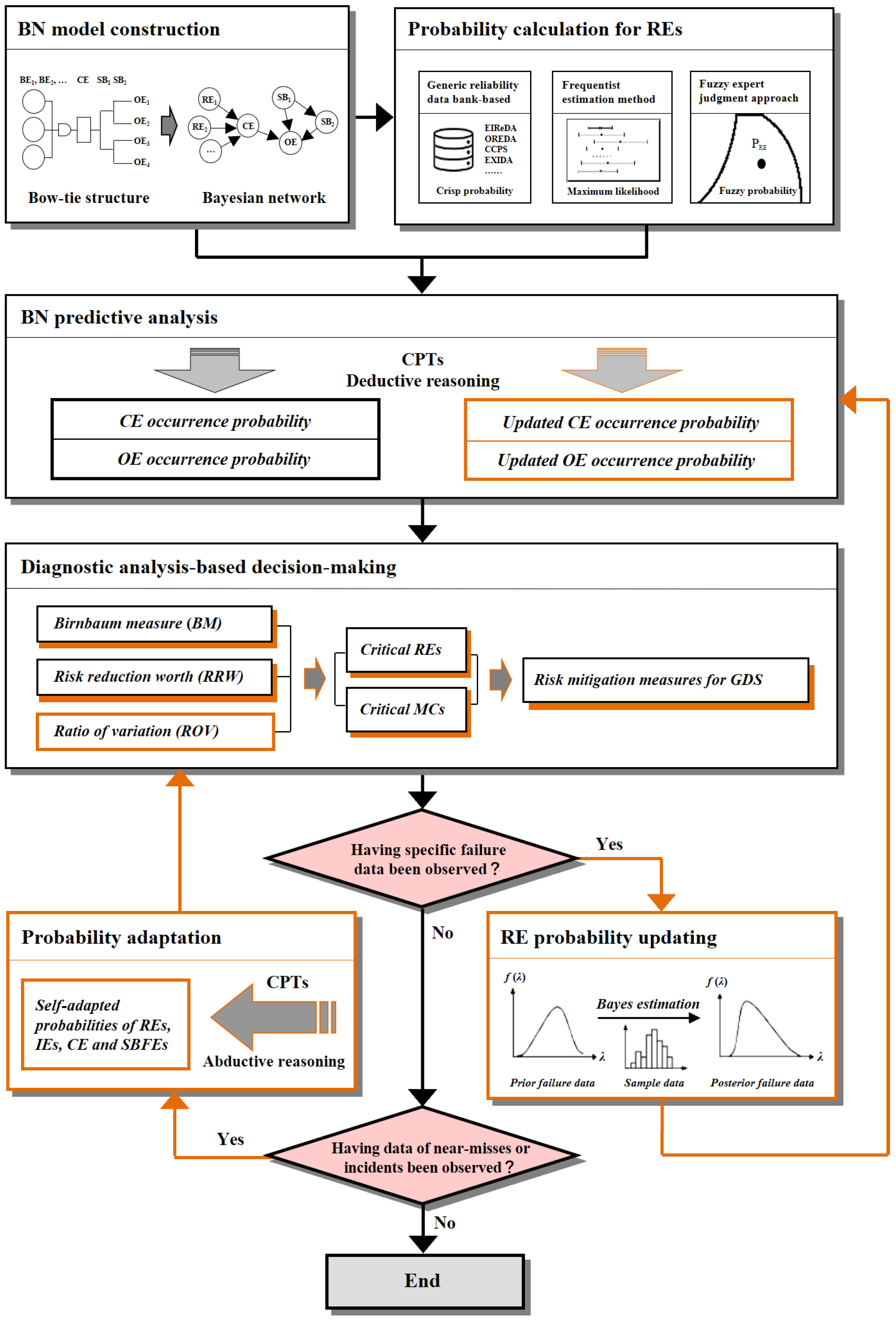
2. Methodology
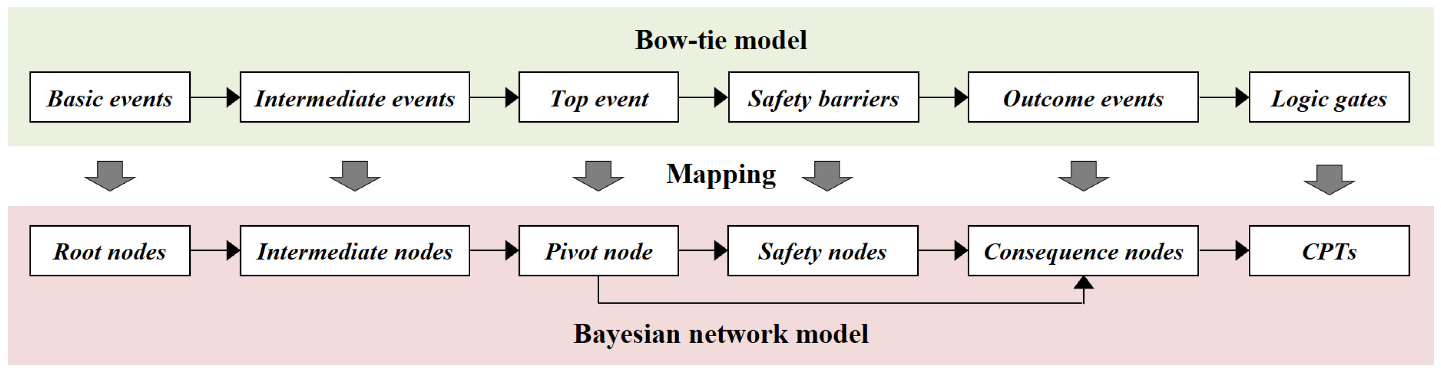
2.1. Accident Model Construction Using Bayesian Network
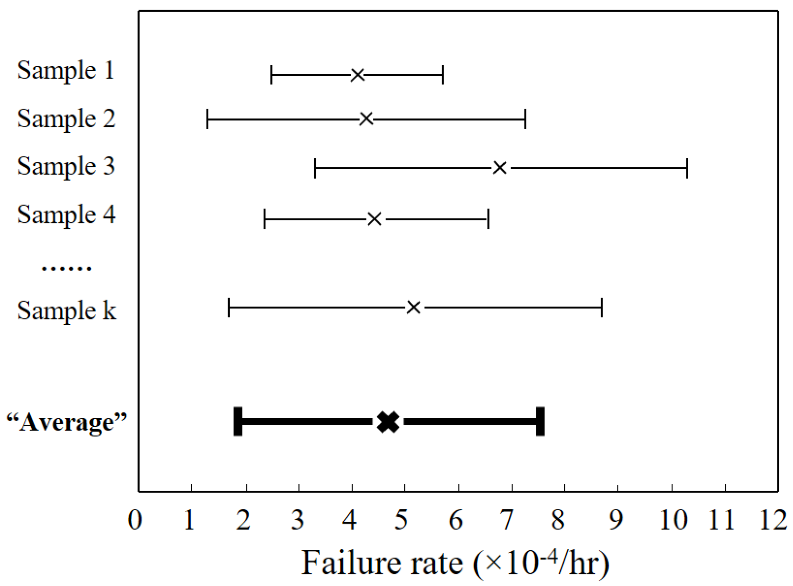
2.2. Probability Estimation Methods for REs
2.2.1. Frequentist Estimation Methods
2.2.2. Fuzzy Set Theory-Based Expert Judgment Method
- Evaluate the likelihood of occurrence for each RE using natural language terms.
- Convert the experts’ linguistic assessments into fuzzy numbers to quantify their subjective evaluations.
- Aggregate the individual experts’ assessments into a unified, comprehensive fuzzy possibility score.
- Transform the fuzzy possibility score into a probability value for subsequent analysis or application.
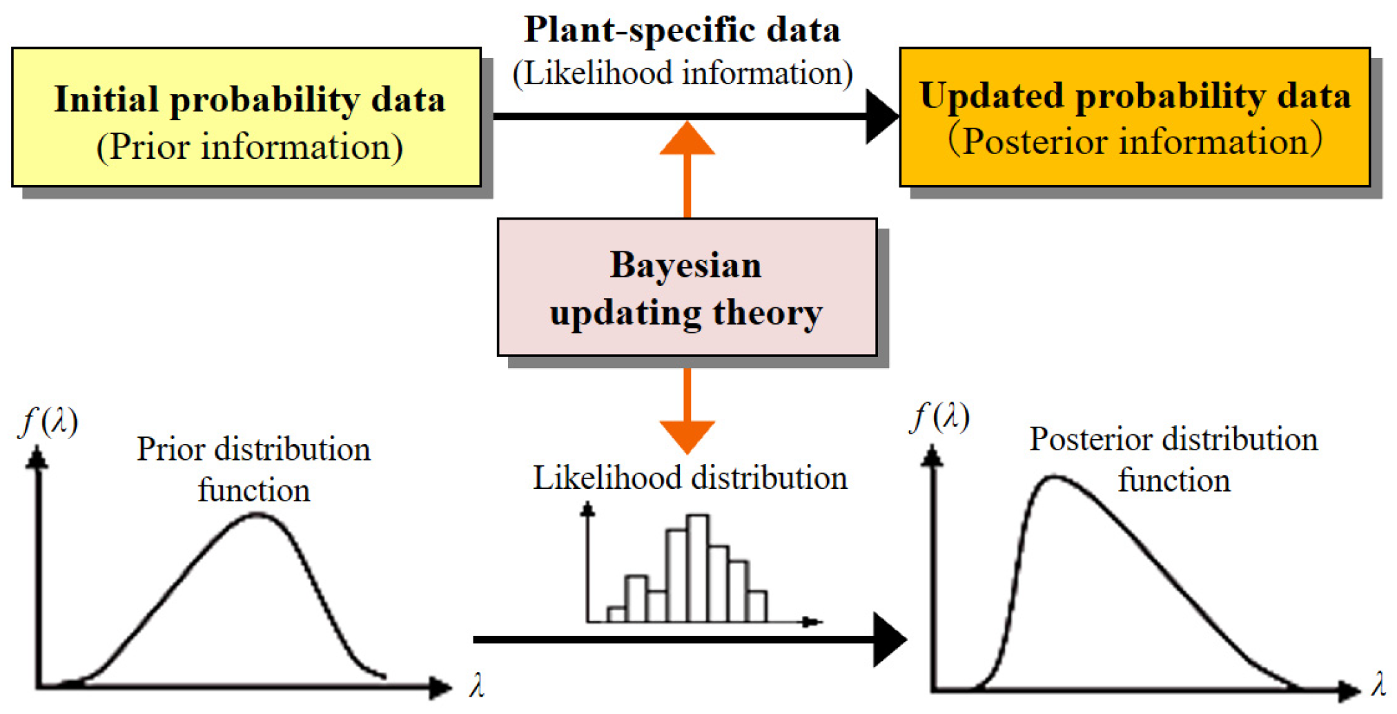
2.3. Dynamic Bayesian Network Analysis
2.3.1. Bayesian Updating Estimation of RE Probabilities
2.3.2. Predictive Analysis
2.3.3. Probability Adaptation
2.3.4. Diagnostic Analysis
3. Application of the Methodology
3.1. Constructing a Bayesian Network Model for GDS Accident Scenarios
3.2. Calculating Prior Probabilities of REs, CE, and OEs
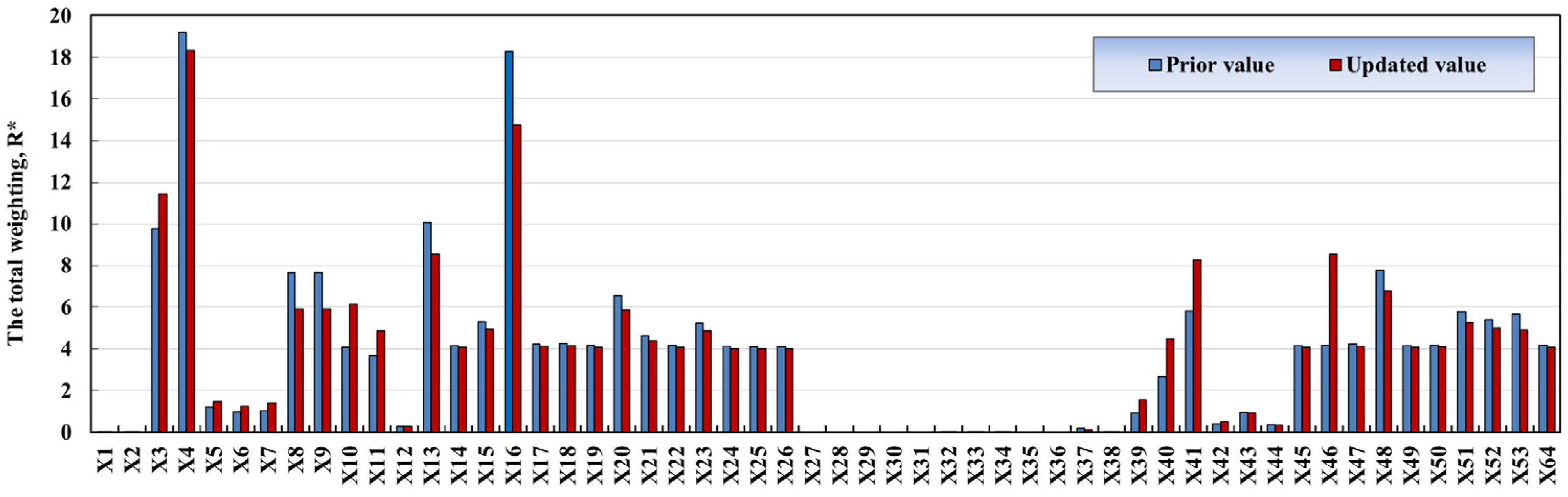
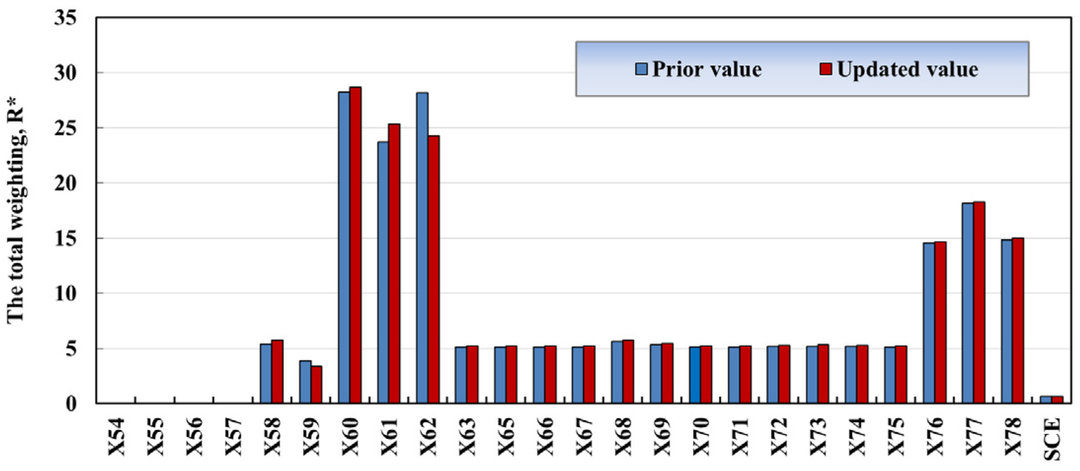
3.3. Determining Contributions of REs to GDS Accident
3.4. Updating Probabilities and Impact Contributions of REs
3.5. Adapting Probabilities for Accident Cause Diagnosis
3.6. Practical and Managerial Implications
- Prioritize Critical Components: The importance measures (e.g., BM, RRW) identify high-risk REs (e.g., X4: non-compliance with operating procedures, X60: automatic emergency cut-off controller failure), enabling targeted inspections and resource allocation.
- Real-Time Risk Mitigation: Integration with GDS integrity management platforms allows automatic updates using new failure data. For instance, if X60’s failure probability increases, maintenance teams can immediately inspect controller units or schedule replacements.
- Adaptive Maintenance Plans: The probability adaptation feature (Section 2.3.3) refines maintenance schedules based on near-misses. For example, a leakage incident triggers adjustments to RE probabilities, highlighting vulnerabilities in corrosion detection (X37) or valve integrity (X55), prompting preemptive repairs.
- Regulatory Compliance: Updated UE probabilities (e.g., CE: 6.18 × 10⁻² post-update) provide quantifiable metrics to ensure compliance with safety thresholds, avoiding penalties and enhancing public trust.
4. Conclusions
4.1. Theoretical Contributions
- By integrating Bayesian network technology, fuzzy expert judgment, and Bayesian updating methods, the framework addresses data uncertainty challenges in safety assessments. Unlike existing approaches limited to unidirectional updates (e.g., backward diagnosis), this framework uniquely supports both forward dynamic prediction (updating UE probabilities with new RE data) and backward dynamic adaptation (adjusting RE probabilities based on observed incidents), enabling comprehensive risk-evolution analysis.
- A novel scenario-deduction model explicitly maps the causal chain from root events (e.g., X4: procedural non-compliance) to critical events (CE: gas leakage) and outcome events (e.g., OE6: long-duration jet fires). This model fills a gap in prior studies by systematically quantifying dynamic interactions among risk factors.
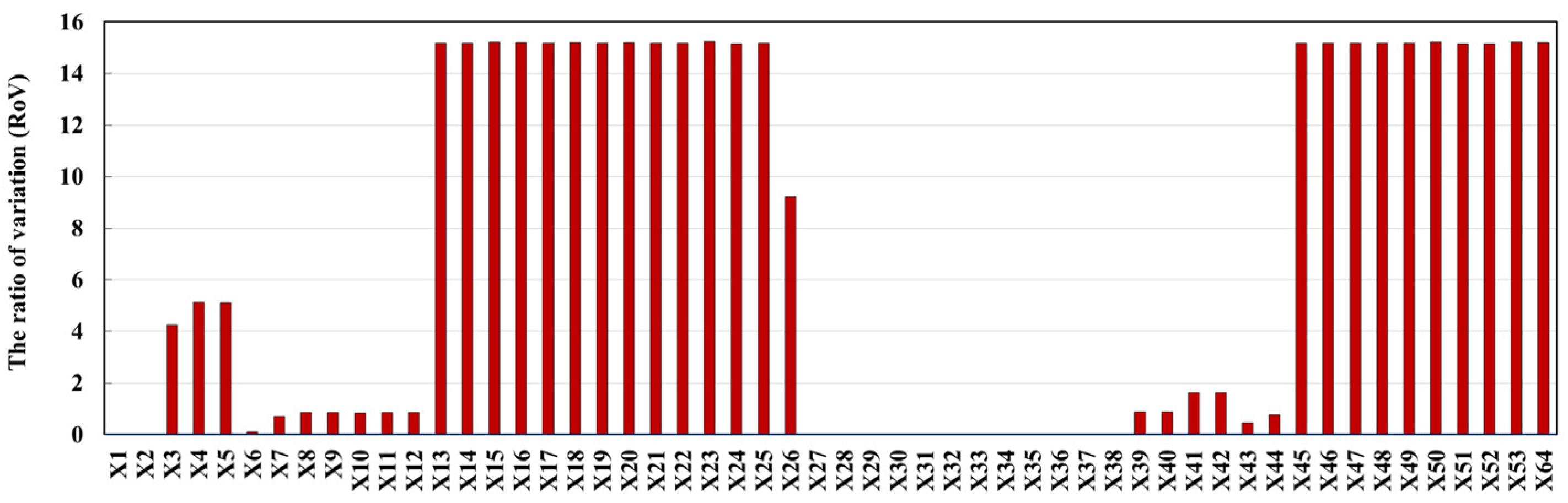
- The introduction of the RoV (ratio of variation) and hybrid importance measures (BM, RRW) establishes a quantifiable linkage between component-level failures and system-level risks, enhancing the precision of causal inference under uncertainty.
4.2. Practical Contributions
- Real-time updates of RE probabilities (e.g., X6’s probability increasing from 9.57 × 10⁻² to 1.69 × 10⁻¹ in Table 4) enable operators to prioritize inspections on high-risk components.
- Updated UE probabilities (e.g., CE: 6.18 × 10⁻²) provide quantifiable metrics to align with safety thresholds, avoiding regulatory penalties and enhancing public trust in GDS operations.
- Integration with GDS integrity management platforms automates risk alerts (e.g., triggering controller replacements when X60 exceeds 3.0 × 10⁻¹), transforming reactive protocols into adaptive strategies.
- Diagnostic analysis (Section 3.3, Section 3.4 and Section 3.5) identifies non-critical REs (e.g., X29: internal coating peeling), allowing operators to reallocate maintenance budgets from low-impact areas to high-priority interventions, such as procedural training (X4) and controller redundancy (X60).
4.3. Cross-Regional Application Expansion
4.4. Future Work
Author Contributions
Funding
Institutional Review Board Statement
Informed Consent Statement
Data Availability Statement
Conflicts of Interest
Glossary
| Abbreviation | Full Name | Description |
| BM | Birnbaum measure | Quantifies the importance of a component in preventing system failure. |
| BN | Bayesian network | A graphical representation of variable dependencies for probabilistic reasoning. |
| BT | Bow-tie | A visual risk-management map linking top events to their causes and consequences. |
| BTA | Bow-tie analysis | An analysis technique that identifies, assesses, and mitigates risks through a bow-tie diagram. |
| CE | Critical event | An event with a major impact on the safety, performance, or reliability of a system. |
| CPT | Conditional probability table | Specifies conditional distribution of a variable based on other variables’ values in a Bayesian network. |
| ETA | Event tree analysis | Identifies and evaluates event sequences leading to specific outcomes in risk assessment. |
| FST | Fuzzy set theory | A mathematical framework for representing partial set membership, capturing degrees of truth. |
| FTA | Fault tree analysis | A top-down analysis of component failures that can lead to system failure. |
| GDS | Gas distribution station | A facility for the safe and stable distribution of natural gas to long-distance pipeline users. |
| ID | Importance degree | A measure of the significance of a component or event to overall performance or safety. |
| IE | Intermediate event | An event that occurs between a root event and an outcome event in a Bayesian network analysis. |
| OE | Outcome event | A node in a Bayesian network signifying the system outcome based on the event sequence. |
| PRA | Probabilistic risk assessment | A risk assessment method that quantifies likelihood and consequences to aid decision-making. |
| QRA | Quantitative risk assessment | Quantifies risk by estimating the probabilities and impacts of potential hazards. |
| RAD | Relative agreement degree | A measure of consensus among individuals or groups on a specific issue, decision, or assessment. |
| RE | Root event | The initiating or fundamental event in a Bayesian network, from which other events are derived. |
| RoV | Ratio of variation | A metric assessing REs’ significance in GDS by comparing pre- and post-RE probability shifts. |
| RRW | Risk reduction worth | A measure ranking REs by criticality and risk impact significance. |
| SB | Safety barrier | A measure mitigating or preventing undesired events and hazards. |
| SBFE | Safety barrier failure event | A safety barrier malfunction that may elevate risk or cause unintended consequences. |
| SCE | Spatial confinement event | Gas accumulation in confined spaces due to environmental constraints. |
| UE | Undesired event | An event that is not intended or desired, often leading to harm, loss, or negative consequences. |
References
- Brogan, M.J. Evaluating risk and natural gas pipeline safety. Politics Policy 2017, 45, 657–680. [Google Scholar] [CrossRef]
- Dong, Y.H.; Yu, D.T. Estimation of failure probability of oil and gas transmission pipelines by fuzzy fault tree analysis. J. Loss Prev. Process Ind. 2005, 18, 83–88. [Google Scholar]
- Kabir, G.; Sadiq, R.; Tesfamariam, S. A fuzzy Bayesian belief network for safety assessment of oil and gas pipelines. Struct. Infrastruct. Eng. 2016, 12, 874–889. [Google Scholar] [CrossRef]
- Markowski, A.S.; Mannan, M.S. Fuzzy logic for piping risk assessment (pfLOPA). J. Loss Prev. Process Ind. 2009, 22, 921–927. [Google Scholar] [CrossRef]
- Shan, K.; Shuai, J.; Xu, K.; Zheng, W. Failure probability assessment of gas transmission pipelines based on historical failur+related data and modification factors. J. Nat. Gas Sci. Eng. 2018, 52, 356–366. [Google Scholar] [CrossRef]
- Bajcar, T.; Cimerman, F.; Širok, B. Model for quantitative risk assessment on naturally ventilated metering-regulation stations for natural gas. Saf. Sci. 2014, 64, 50–59. [Google Scholar] [CrossRef]
- Wang, D.; Liang, P.; Yu, Y.; Fu, X.; Hu, L. An integrated methodology for assessing accident probability of natural gas distribution station with data uncertainty. J. Loss Prev. Process Ind. 2019, 62, 103941. [Google Scholar] [CrossRef]
- Zarei, E.; Azadeh, A.; Khakzad, N.; Aliabadi, M.M.; Mohammadfam, I. Dynamic safety assessment of natural gas stations using Bayesian network. J. Hazard. Mater. 2017, 321, 830–840. [Google Scholar] [CrossRef]
- Lavasani, S.M.; Zendegani, A.; Celik, M. An extension to Fuzzy Fault Tree Analysis (FFTA) application in petrochemical process industry. Process Saf. Environ. Prot. 2015, 93, 75–88. [Google Scholar] [CrossRef]
- Wang, D.; Zhang, P.; Chen, L. Fuzzy fault tree analysis for fire and explosion of crude oil tanks. J. Loss Prev. Process Ind. 2013, 26, 1390–1398. [Google Scholar] [CrossRef]
- Ferdous, R.; Khan, F.; Sadiq, R.; Amyotte, P.; Veitch, B. Veitch Handling data uncertainties in event tree analysis. Process Saf. Environ. Prot. 2009, 87, 283–292. [Google Scholar] [CrossRef]
- Ramzali, N.; Lavasani, M.R.M.; Ghodousi, J. Safety barriers analysis of offshore drilling system by employing Fuzzy Event Tree Analysis. Saf. Sci. 2015, 78, 49–59. [Google Scholar] [CrossRef]
- Ferdous, R.; Khan, F.; Sadiq, R.; Amyotte, P.; Veitch, B. Analyzing system safety and risks under uncertainty using a bow-tie diagram: An innovative approach. Process Saf. Environ. Prot. 2013, 91, 1–18. [Google Scholar] [CrossRef]
- Shahriar, A.; Sadiq, R.; Tesfamariam, S. Risk analysis for oil & gas pipelines: A sustainability assessment approach using fuzzy based bow-tie analysis. J. Loss Prev. Process Ind. 2012, 25, 505–523. [Google Scholar]
- Rathnayaka, S.; Khan, F.; Amyotte, P. SHIPP methodology: Predictive accident modeling approach. Part I: Methodology and model description. Process Saf. Environ. Prot. 2011, 89, 151–164. [Google Scholar] [CrossRef]
- Landquist, H.; Rosén, L.; Lindhe, A.; Norberg, T.; Hassellöv, I.-M. Hassellöv Bayesian updating in a fault tree model for shipwreck risk assessment. Sci. Total Environ. 2017, 590, 80–91. [Google Scholar] [CrossRef]
- Khakzad, N.; Khan, F.; Amyotte, P. Dynamic risk analysis using bow-tie approach. Reliab. Eng. Syst. Saf. 2012, 104, 36–44. [Google Scholar] [CrossRef]
- Ahmed, S.; Li, T.; Huang, S.; Cao, J. Dynamic and quantitative risk assessment of Cruise ship pod propulsion system failure: An integrated Type-2 Fuzzy-Bayesian approach. Ocean Eng. 2023, 279, 114601. [Google Scholar] [CrossRef]
- Cai, B.; Fan, H.; Shao, X.; Liu, Y.; Liu, G.; Liu, Z.; Ji, R. Remaining useful life re-prediction methodology based on Wiener process: Subsea Christmas tree system as a case study. Comput. Ind. Eng. 2020, 151, 106983. [Google Scholar] [CrossRef]
- Fan, H.H.; Enshaei, S.G. Jayasinghe Dynamic quantitative risk assessment of LNG bunkering SIMOPs based on Bayesian network. J. Ocean Eng. Sci. 2023, 8, 508–526. [Google Scholar] [CrossRef]
- Liu, Z.; Ma, Q.; Shi, X.; Chen, Q.; Han, Z.; Cai, B.; Liu, Y. A dynamic quantitative risk assessment method for drilling well control by integrating multi types of risk factors. Process Saf. Environ. Prot. 2022, 167, 162–172. [Google Scholar] [CrossRef]
- Yazdi, M.; Kabir, S. A fuzzy Bayesian network approach for risk analysis in process industries. Process Saf. Environ. Prot. 2017, 111, 507–519. [Google Scholar] [CrossRef]
- Zarei, E.; Khakzad, N.; Cozzani, V.; Reniers, G. Safety analysis of process systems using Fuzzy Bayesian Network (FBN). J. Loss Prev. Process Ind. 2019, 57, 7–16. [Google Scholar] [CrossRef]
- Zong, S.; Wang, Z.; Liu, K.; Wang, G.; Lu, Y.; Huang, T. Risk assessment of general FPSO supply system based on hybrid fuzzy fault tree and Bayesian network. Ocean Eng. 2024, 311, 118767. [Google Scholar] [CrossRef]
- Mahmood, Y.; Chen, J.; Yodo, N.; Huang, Y. Optimizing natural gas pipeline risk assessment using hybrid fuzzy bayesian networks and expert elicitation for effective decision-making strategies. Gas Sci. Eng. 2024, 125, 205283. [Google Scholar] [CrossRef]
- Sinaki, Y.Y.; Baradaran, S.; Gilani, N. Insight process safety of a hydrogen turbine supply system: A comprehensive dynamic risk assessment using a fuzzy Bayesian network. Int. J. Hydrogen Energy 2024, 89, 474–485. [Google Scholar] [CrossRef]
- Wang, Q.-A.; Chen, J.; Ni, Y.; Xiao, Y.; Liu, N.; Liu, S.; Feng, W. Application of Bayesian networks in reliability assessment: A systematic literature review. Structures 2025, 71, 108098. [Google Scholar] [CrossRef]
- Khakzad, N.; Khan, F.; Amyotte, P. Dynamic safety analysis of process systems by mapping bow-tie into Bayesian network. Process Saf. Environ. Prot. 2013, 91, 46–53. [Google Scholar] [CrossRef]
- SINTEF Industrial Management. Offshore Reliability Data Handbook; Oreda Participants: Stavanger, Norway, 2015. [Google Scholar]
- Exida, L. Safety Equipment Reliability Handbook; Exida: Sellesville, PA, USA, 2005. [Google Scholar]
- Center for Chemical Process Safety (CCPS). Guidelines for Process Equipment Reliability Data, with Data Tables, 1st ed.; American Institute of Chemical Engineers, CCPS: New York, NY, USA, 1989. [Google Scholar]
- Atwood, C.; LaChance, J.; Martz, H.; Anderson, D.; Englehardt, M.; Whitehead, D.; Wheeler, T. Handbook of Parameter Estimation for Probabilistic Risk Assessment; US Nuclear Regulatory Commission: Rockville, MD, USA, 2003. [Google Scholar]
- Zhang, L.; Wu, X.; Skibniewski, M.J.; Zhong, J.; Lu, Y. Bayesian-network-based safety risk analysis in construction projects. Reliab. Eng. Syst. Saf. 2014, 131, 29–39. [Google Scholar] [CrossRef]


| RE | Description | Prior Probability | RE | Description | Prior Probability |
|---|---|---|---|---|---|
| X1 | Improper inspection and maintenance | 2.47 × 10⁻³ | X41 | Vent valve of pig trap failure | 4.67 × 10⁻² |
| X2 | Solid impurities in natural gas | 1.90 × 10⁻⁴ | X42 | Pig indicator failed | 8.00 × 10⁻⁴ |
| X3 | Separator outlet valve fails to shutdown | 2.70 × 10⁻² | X43 | Safety valve fails to active | 1.70 × 10⁻² |
| X4 | Non-compliance with operating procedure | 4.50 × 10⁻² | X44 | Gas erosion abrasion | 2.37 × 10⁻³ |
| X5 | Non-professional operation | 4.30 × 10⁻⁴ | X45 | Seal failure of blind plate | 1.70 × 10⁻⁴ |
| X6 | Separator drain valve fails to open | 9.57 × 10⁻² | X46 | Flange gasket breakage | 4.32 × 10⁻³ |
| X7 | Separator inlet valve fails to close | 3.12 × 10⁻² | X47 | Improper selection of flange gasket | 2.30 × 10⁻⁴ |
| X8 | Separator inlet pressure gauge failure | 8.64 × 10⁻² | X48 | Flange gasket aging | 2.69 × 10⁻³ |
| X9 | Separator pressure gauge failure | 8.64 × 10⁻² | X49 | Flange connection bolt failure | 1.70 × 10⁻⁴ |
| X10 | Separator manual vent valve failure | 4.67 × 10⁻² | X50 | Poor installation quality | 1.90 × 10⁻⁴ |
| X11 | Separator high pressure alarm failure | 4.22 × 10⁻² | X51 | Valve body defect | 1.30 × 10⁻³ |
| X12 | No human response to high voltage alarm | 8.00 × 10⁻⁴ | X52 | Seal packing failure | 1.04 × 10⁻³ |
| X13 | Seal ring of manhole cover failure | 4.32 × 10⁻³ | X53 | Poor seal between valve body and cover | 9.50 × 10⁻⁴ |
| X14 | Fastening bolt of manhole cover failure | 1.70 × 10⁻⁴ | X54 | Artificial blockage leakage point failure | 2.50 × 10⁻² |
| X15 | Equipment material defect | 9.80 × 10⁻⁴ | X55 | Automatic ball valve fails to close | 1.18 × 10⁻² |
| X16 | Equipment manufacturing defect | 1.00 × 10⁻² | X56 | Manual shutdown valve failure | 1.31 × 10⁻³ |
| X17 | Insufficient strength design | 2.30 × 10⁻⁴ | X57 | No response to manual valve | 4.00 × 10⁻² |
| X18 | Calculation method error | 2.50 × 10⁻⁴ | X58 | Automatic emergency shut−off valve failure | 4.67 × 10⁻² |
| X19 | Outdated design specifications | 1.80 × 10⁻⁴ | X59 | Automatic emergency cut−off sensor failure | 2.89 × 10⁻² |
| X20 | Poor coating repair | 1.84 × 10⁻³ | X60 | Automatic emergency cut−off controller failure | 2.50 × 10⁻¹ |
| X21 | Material damaged in handling | 4.90 × 10⁻⁴ | X61 | Manual emergency cut−off valve failure | 3.12 × 10⁻² |
| X22 | Material damage during installation | 1.80 × 10⁻⁴ | X62 | No response to manual emergency valve | 4.00 × 10⁻² |
| X23 | Weld defect | 9.30 × 10⁻⁴ | X63 | Lightning spark | 1.80 × 10⁻⁴ |
| X24 | Earthquake | 1.30 × 10⁻⁴ | X64 | Accidental external impact | 1.81 × 10⁻⁴ |
| X25 | Flood | 1.20 × 10⁻⁴ | X65 | Sparks caused by short circuit | 1.80 × 10⁻⁴ |
| X26 | Subsidence | 1.20 × 10⁻⁴ | X66 | Non−explosion−proof monitoring equipment | 1.80 × 10⁻⁴ |
| X27 | Corrosion inhibitor failure | 5.10 × 10⁻⁴ | X67 | Other non−explosion−proof electrical appliances | 2.20 × 10⁻⁴ |
| X28 | Inner coating thinning | 9.60 × 10⁻⁴ | X68 | Clothing friction electrification | 1.95 × 10⁻³ |
| X29 | Internal coating peeling | 9.80 × 10⁻⁴ | X69 | Other electrostatic | 9.80 × 10⁻⁴ |
| X30 | With water | 1.22 × 10⁻³ | X70 | Station domestic fire | 1.90 × 10⁻⁴ |
| X31 | Acid medium | 2.30 × 10⁻⁴ | X71 | Smoking | 1.10 × 10⁻⁴ |
| X32 | Harsh environment | 1.90 × 10⁻⁴ | X72 | Vehicles not fitted with spark arrestor | 4.20 × 10⁻⁴ |
| X33 | Outer coating thinning | 1.32 × 10⁻³ | X73 | Friction at the leak | 4.80 × 10⁻⁴ |
| X34 | Outer coating peeling | 1.66 × 10⁻³ | X74 | High speed collisions of solid impurities | 4.60 × 10⁻⁴ |
| X35 | Residual stress | 1.80 × 10⁻⁴ | X75 | Tool impact sparks | 1.30 × 10⁻⁴ |
| X36 | Stress concentration | 1.90 × 10⁻⁴ | X76 | Hot work without permission | 3.30 × 10⁻² |
| X37 | Lack of periodic corrosion detection | 5.00 × 10⁻² | X77 | Not following hot work permit | 4.50 × 10⁻² |
| X38 | Corrosion detection instrument failure | 2.40 × 10⁻⁴ | X78 | Insufficient supervision | 3.40 × 10⁻² |
| X39 | Electric ball valve of pig trap outlet fails to open | 1.18 × 10⁻² | SCE | Spatial confinement event | 1.21 × 10⁻⁴ |
| X40 | Drain valve of pig traps fails to close | 3.86 × 10⁻² |
| Parameter | Values | Parameter | Values |
|---|---|---|---|
| n1 | 1 failures | τ1 | 43,800 h |
| n2 | 0 failures | τ2 | 26,280 h |
| n3 | 1 failures | τ3 | 61,320 h |
| n4 | 0 failures | τ4 | 43,800 h |
| 1.14 × 10⁻⁵ | 1.09 × 10⁻⁵ | ||
| S1 | 1.75 × 10⁵ | 7.90 × 10⁴ | |
| S2 | 8.29 × 10⁹ | 8.63 × 10⁻¹ | |
| ν | 1.63 × 10⁻⁵ | θ0.05 | 6.52 × 10⁻⁷ |
| 1.38 × 10⁻¹⁰ | θ0.95 | 3.79 × 10⁻⁵ | |
| = (6.52 × 10⁻⁷, 1.09 × 10⁻⁵, 3.79 × 10⁻⁵) hr−1 = (5.63 × 10⁻³, 9.57 × 10⁻², 3.28 × 10⁻¹) yr−1 | |||
| Undesired Event | Description | Prior Probability |
|---|---|---|
| CE | Natural gas release from GDS | 5.23 × 10⁻² |
| OE1 | Minor material losses | 4.54 × 10⁻² |
| OE2 | Flash-fire | 6.98 × 10⁻⁷ |
| OE3 | Short-duration jet fire | 5.77 × 10⁻³ |
| OE4 | Major material losses | 9.93 × 10⁻⁴ |
| OE5 | Vapor cloud explosion | 1.53 × 10⁻⁸ |
| OE6 | Long-duration jet fire | 1.26 × 10⁻⁴ |
| RE | Cumulative Plant-Specific Failure Data | Number of Samples | Updated Probability | UE | Updated Probability |
|---|---|---|---|---|---|
| X3 | 2 times within 56,160 h | 8 | 3.34 × 10⁻² | CE | 6.18 × 10⁻² |
| X6 | 1 times within 17,520 h | 2 | 1.69 × 10⁻¹ | OE1 | 5.35 × 10⁻² |
| X7 | 0 times within 105,500 h | 8 | 2.42 × 10⁻² | OE2 | 8.22 × 10⁻⁷ |
| X10 | 1 times within 73,270 h | 8 | 8.94 × 10⁻² | OE3 | 6.80 × 10⁻³ |
| X11 | 1 times within 73,270 h | 8 | 7.17 × 10⁻² | OE4 | 1.34 × 10⁻³ |
| X39 | 1 times within 87,640 h | 10 | 2.12 × 10⁻² | OE5 | 2.06 × 10⁻⁸ |
| X40 | 1 times within 98,480 h | 10 | 6.38 × 10⁻² | OE6 | 1.70 × 10⁻⁴ |
| X41 | 1 times within 121,040 h | 10 | 6.43 × 10⁻² | ||
| X43 | 1 times within 103,680 h | 12 | 2.45 × 10⁻² | ||
| X55 | 1 times within 141,080 h | 12 | 1.99 × 10⁻² | ||
| X56 | 1 times within 109,820 h | 10 | 4.11 × 10⁻³ | ||
| X58 | 1 times within 165,600 h | 14 | 4.93 × 10⁻² | ||
| X59 | 0 times within 146,300 h | 14 | 2.22 × 10⁻² | ||
| X61 | 1 times within 107,900 h | 10 | 4.24 × 10⁻² |
| RE | Adapted Probability | RE | Adapted Probability | RE | Adapted Probability |
|---|---|---|---|---|---|
| X1 | 2.47 × 10⁻³ | X19 | 2.91 × 10⁻³ | X37 | 5.17 × 10⁻² |
| X2 | 1.92 × 10⁻⁴ | X20 | 2.98 × 10⁻² | X38 | 2.48 × 10⁻⁴ |
| X3 | 1.75 × 10⁻¹ | X21 | 7.93 × 10⁻³ | X39 | 3.99 × 10⁻² |
| X4 | 2.75 × 10⁻¹ | X22 | 2.91 × 10⁻³ | X40 | 1.20 × 10⁻¹ |
| X5 | 2.62 × 10⁻³ | X23 | 1.51 × 10⁻² | X41 | 1.68 × 10⁻¹ |
| X6 | 1.83 × 10⁻¹ | X24 | 2.10 × 10⁻³ | X42 | 2.09 × 10⁻³ |
| X7 | 4.11 × 10⁻² | X25 | 1.94 × 10⁻³ | X43 | 3.57 × 10⁻² |
| X8 | 1.60 × 10⁻¹ | X26 | 1.94 × 10⁻³ | X44 | 4.17 × 10⁻³ |
| X9 | 1.60 × 10⁻¹ | X27 | 5.10 × 10⁻⁴ | X45 | 2.75 × 10⁻² |
| X10 | 1.65 × 10⁻¹ | X28 | 9.60 × 10⁻⁴ | X46 | 6.99 × 10⁻² |
| X11 | 1.33 × 10⁻¹ | X29 | 9.80 × 10⁻⁴ | X47 | 3.72 × 10⁻³ |
| X12 | 1.48 × 10⁻³ | X30 | 1.22 × 10⁻³ | X48 | 4.35 × 10⁻² |
| X13 | 6.99 × 10⁻² | X31 | 2.30 × 10⁻⁴ | X49 | 2.75 × 10⁻³ |
| X14 | 2.75 × 10⁻³ | X32 | 1.90 × 10⁻⁴ | X50 | 3.08 × 10⁻³ |
| X15 | 1.59 × 10⁻² | X33 | 1.32 × 10⁻³ | X51 | 2.10 × 10⁻² |
| X16 | 1.62 × 10⁻¹ | X34 | 1.66 × 10⁻³ | X52 | 1.68 × 10⁻² |
| X17 | 3.72 × 10⁻³ | X35 | 1.80 × 10⁻⁴ | X53 | 1.54 × 10⁻² |
| X18 | 4.05 × 10⁻³ | X36 | 1.90 × 10⁻⁴ | X64 | 2.93 × 10⁻² |
Disclaimer/Publisher’s Note: The statements, opinions and data contained in all publications are solely those of the individual author(s) and contributor(s) and not of MDPI and/or the editor(s). MDPI and/or the editor(s) disclaim responsibility for any injury to people or property resulting from any ideas, methods, instructions or products referred to in the content. |
© 2025 by the authors. Licensee MDPI, Basel, Switzerland. This article is an open access article distributed under the terms and conditions of the Creative Commons Attribution (CC BY) license (https://creativecommons.org/licenses/by/4.0/).
Share and Cite
Wang, D.; Huang, H.; Wang, B.; Tian, S.; Liang, P.; Yu, W. A Dynamic Assessment Methodology for Accident Occurrence Probabilities of Gas Distribution Station. Appl. Sci. 2025, 15, 4464. https://doi.org/10.3390/app15084464
Wang D, Huang H, Wang B, Tian S, Liang P, Yu W. A Dynamic Assessment Methodology for Accident Occurrence Probabilities of Gas Distribution Station. Applied Sciences. 2025; 15(8):4464. https://doi.org/10.3390/app15084464
Chicago/Turabian StyleWang, Daqing, Huirong Huang, Bin Wang, Shaowei Tian, Ping Liang, and Weichao Yu. 2025. "A Dynamic Assessment Methodology for Accident Occurrence Probabilities of Gas Distribution Station" Applied Sciences 15, no. 8: 4464. https://doi.org/10.3390/app15084464
APA StyleWang, D., Huang, H., Wang, B., Tian, S., Liang, P., & Yu, W. (2025). A Dynamic Assessment Methodology for Accident Occurrence Probabilities of Gas Distribution Station. Applied Sciences, 15(8), 4464. https://doi.org/10.3390/app15084464