Abstract
The paper presents an innovative matrix method for defect analysis in heterogeneous structures with significant differences in stiffness parameters. The proposed approach modifies the finite element method (FEM) by introducing a refined type of finite element capable of handling regions with varying material and geometrical properties. Unlike traditional FEM discretization, which increases computational time calculations due to mesh refinement in stiffness-variable areas, the proposed method maintains a consistent discretization while adjusting shape functions to reflect internal stiffness changes. An original functional for modifying linear shape function distributions is introduced, leading to piecewise broken-line shape functions. This enhancement significantly improves the accuracy of numerical calculations, as verified by computational calculations. The explicit formulation of the stiffness matrix enhances computational efficiency, making the approach particularly useful for periodic structures with inclusions, voids, or localized material defects. The results of numerical tests demonstrate that the proposed method provides solutions closely aligned with conventional FEM results while substantially reducing computational costs. The approach is particularly relevant for structural engineering applications where defect analysis and material heterogeneity play a critical role in design and safety evaluation.
1. Introduction
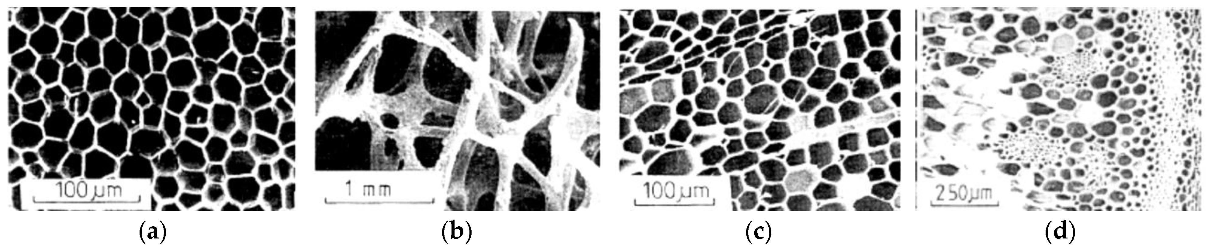
The natural environment and all human products include materials with heterogeneous and variable structure, both at the microscale and macroscale level. As examples, structures created by animate and inanimate nature can be given. In Figure 1, examples of biological structures with a mesh structure filled with biological fluids are presented. In Figure 2, examples of manmade construction materials that contain inclusions with different strength properties are shown. Some materials are heterogeneous due to the production process itself, while others are heterogeneous due to defects and material losses.
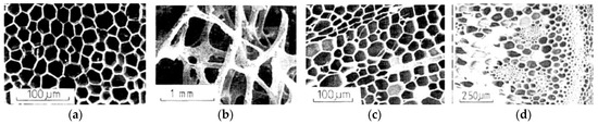
Figure 1.
Natural biological structures: (a) oak bark; (b) cellular bone; (c) balsa wood; (d) plant stem [1].
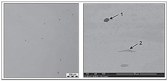
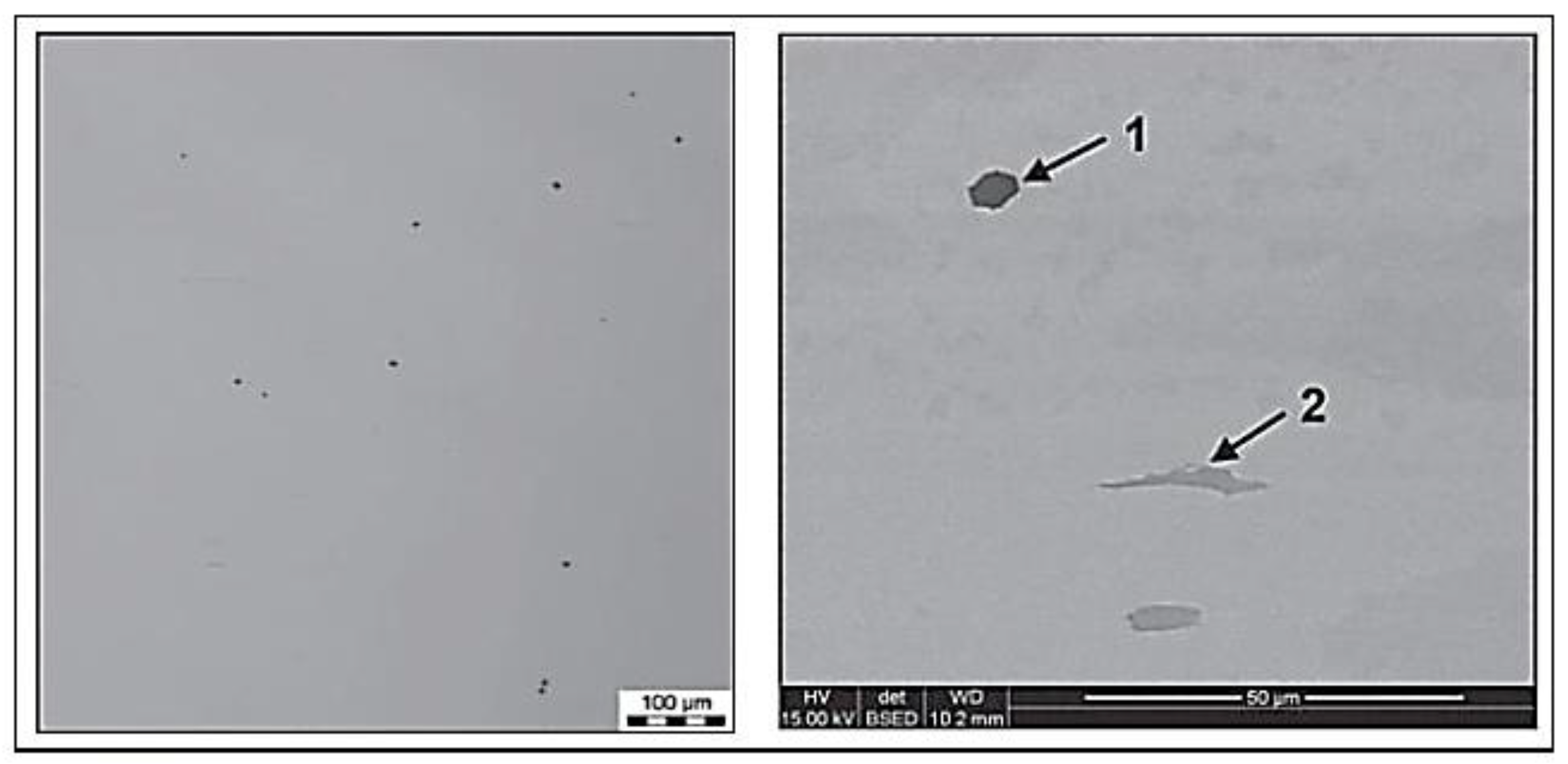
Figure 2.
Non-metallic inclusions in steel [2].
In order to analyze the distribution of internal forces, stress, and deformations in structural elements and materials, the FEM can be used. The method is universal and allows for modeling practically any material and any structure. However, problems related to the computational work involved can be encountered. Specifically, these concern the number of unknowns depending on the number of finite elements. The more complex a structure is, the more unknowns are generated in the computational model. Examples of potential discretization patterns of complex structures are presented in Figure 3.
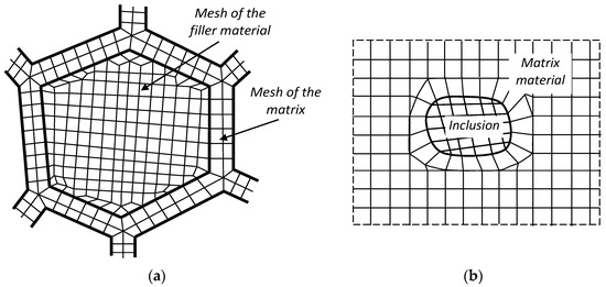
Figure 3.
Examples of standard discretization: (a) bone tissue; (b) single inclusion.
One solution is to use special finite elements, which are dedicated to enabling averaging of parameters at the level of repeatable finite elements. Examples of alternative discretization of structures are shown in Figure 4, where special elements are used. The tendency to describe larger surfaces of structures with single finite elements is quite common in the literature. In the case of masonry structures, the aim is to include entire parts of the wall [3,4,5,6] or to include at least several layers of bricks and mortar [7]. New types of finite elements have been developed specifically to address issues related to the need to take into account the content of inclusions, voids [8], as well as the propagation of cracks [9]. It is also important to consider the time computational calculations and the need for significant computing power of computers. In order to reduce the costs of the computational calculations, optimizations of the calculation procedures are constantly being developed [10].
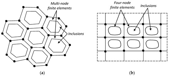
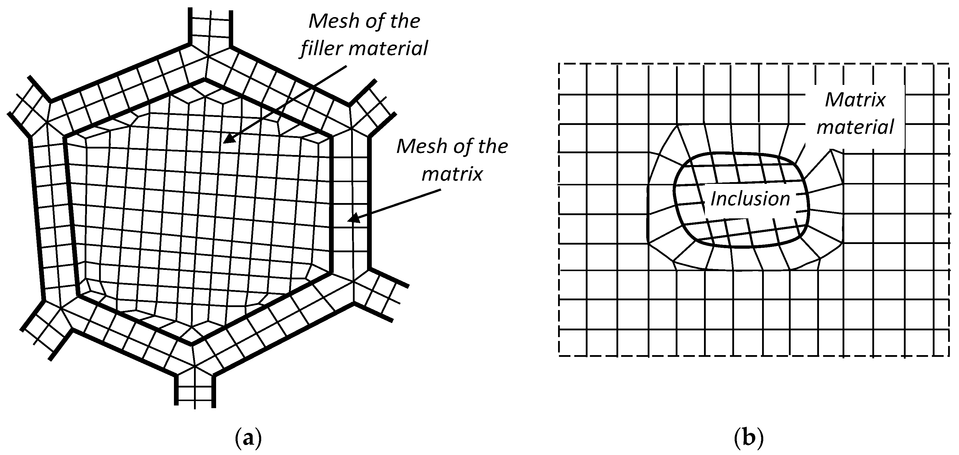
Figure 4.
Example of discretization using special elements: (a) multi-node; (b) four-node.
Heterogeneous materials usually contain various types of inclusions. The influence of inclusions on crack propagation and on increase in failure risk is evident and is often analyzed and studied at various levels, i.e., considering both micro- and macrostructures [11,12,13,14]. A pioneering approach and probably the most important analytical result of micromechanics in the analysis of inclusions is a solution based on the effective approximation of inhomogeneous material developed by Eshelby [15,16]. The heterogeneous material is replaced by homogeneous material with the resultant properties obtained on the basis of an analytical or semi-analytical solution to a boundary mechanics problem. The obtained original, analytical solution concerning the infinite matrix containing an ellipsoidal inclusion was later developed by many other authors [17,18,19]. For example, in [20], based on Eshelby’s formulation, a finite matrix containing an inclusion was analyzed.
The problem of modeling inhomogeneous and porous materials was also analyzed by the authors in [21]. The presented homogenization method for heterogeneous and non-linear materials differs from those described in the literature and is particularly suitable for the calculation of more complex structures. In the case of a non-linear non-homogeneous material, its representative volume element (RVE) and the load space consisting of all boundary conditions to be imposed on the RVE should be considered first.
Another method of homogenization is proposed in [22]. Higher-order FEM has been successfully applied to multi-mesh homogenization of incoherent material. As the authors emphasize in [23], the main achievement is improved representation inside the mesh, what is characteristic for bubble functions. The effect is in the form of rapid, exponential convergence of displacements and stresses in the numerical tests performed in relation to the number of degrees of freedom and the duration of calculations.
In order to perform the two-scale analysis for non-linear heterogeneous materials with periodic microstructure, the authors of [24] introduced a parallel algorithm to achieve the appropriate computational efficiency. Despite the usefulness of the two-scale non-linear method in the analysis of non-linear heterogeneous materials, it was observed that the method is quite computationally demanding. It was decided to increase the computational efficiency by performing microscale analyses on separate PC computers included in the PC set to minimize the transfer of information between individual processors. The numerical examples presented suggest the usefulness of parallel calculations in the analysis of practical problems.
Another way to analyze non-homogeneous materials is the extended multiscale finite element method (EMsFEM). The key factor in the efficiency and accuracy of EMsFEM is the application of numerical basis functions (NBFs). In [25], a general method of constructing basis functions (NBFs) is presented and a generalized isoparametric interpolation based on the rigid displacement properties of these functions is proposed. Theoretical and numerical aspects of the algorithm support the conclusion that computer calculations using EMsFEM are much more efficient than direct solutions. The algorithm has been verified by linear analysis of materials with random impurities and holes, and the efficiency of the method can be improved by parallel calculations.
Finite elements can provide a solution to the problem of rare inclusions (Figure 2). In such cases, it is possible to use regular meshes, where four-node elements are the most effective solution. The use of a regular mesh with four-node elements is common in the analysis of periodic composite structures. An example is the use of eigenelements [26,27,28]. The development and improvement of finite elements is often aimed at reducing the time taken and the computational power while maintaining appropriate accuracy of calculations. In addition, there are issues related to the possibilities and methods of homogenization of heterogeneous but periodic structures, especially when it comes to the previously mentioned multi-scale modeling analysis [29]. Periodic systems are typical, especially for composite materials. An example of analysis involves the use of another type of element, the so-called hierarchical method [30]. In many modifications of finite elements, various types of changes are often introduced concerning the shape functions [31], i.e., the distribution of displacements and stress inside the surface of a two-dimensional element.
An additional contribution to the development of numerical methods was the formulation of the Virtual Element Method (VEM). This extension of the FEM was introduced by Brezzi’s group [32,33] and was addressed mostly to interior problems. Recently VEM was extended also to exterior problems by the Desiderio and Falletta group [34,35]. VEM allows meshes to be considered where elements are of a general shape, and to define local discrete spaces in such a way that the elementary stiffness matrix can be computed using only the degrees of freedom, without need to explicitly recognize the expression of the non-polynomial functions. Hence, arbitrarily high-order VEM can be easily applied by maintaining the simplicity of the implementation.
The paper presents a method where the discretization shown in Figure 4b is used. A concept of defects analysis of heterogenous structures is proposed in the form of application of a modified type of finite element. The method applies particularly to structures which include areas with different stiffness parameters. It concerns structures made of different materials, consisting of parts with variable thickness or parts with various defects. In order to reduce the number of elements in the FEM numerical model, discretization can be applied regardless of stiffness parameter changes. As a result, the single finite element includes areas with various geometrical or material parameters. It is recognized that the stiffness distribution inside the finite element has an impact on the approximation function of the strain field inside the element. The use of broken shape functions allows for a significant reduction in the number of finite elements required to perform the FEM calculations.
2. Materials and Methods
2.1. Formulation of Two-Dimensional Multi-Area Finite Elements. Theoretical Assumptions
The use of shape functions enables a matrix definition of a finite element. In structural modeling applications, finite elements are implemented to represent material characteristics, assuming a linear relationship between strain and stress. Therefore, the basic FEM equations leading to the determination of the finite element stiffness matrix Ke have the following form:
where —matrix of differential operators,
—shape function matrix,
—strain matrix,
—material characteristic matrix,
—Jacobi matrix,
V—volume of the element.
Determination of the stiffness matrix of the finite element described by Equation (4) can be performed as follows:
- explicit, i.e., by analytical integration of the expression (4); in this way, the so-called explicit forms of the stiffness matrix are obtained in the form of formulas; explicit forms of the stiffness matrix are the most effective form of element matrix in computational analyses; however, difficulties arise related to their obtaining limit applications to the simplest elements of regular shapes (bar elements, two-dimensional rectangular elements, etc.);
- implicit, i.e., by numerical integration of the expression (4); in this way the stiffness matrix is obtained directly in numerical form; the Gauss–Legendre formula is often used and allows changing the integral expression into a summation expression; for example, for a function of one variable:where n is the number of integration points (so-called Gauss points), and and denote the weight and the value of the integrand function at the i-th integration point, respectively.
2.2. Stiffness Matrix Formulation for Four-Node Element
The conception of multi-area elements, based on the example of one-dimensional finite elements, was presented in [36], where verification tests were carried out using the example of a one-dimensional finite element with linear and broken shape functions. The tests performed confirmed the correctness of the assumptions and showed that it is possible to increase the accuracy of the solution up to 100%, i.e., to achieve an exact solution (called the reference solution).
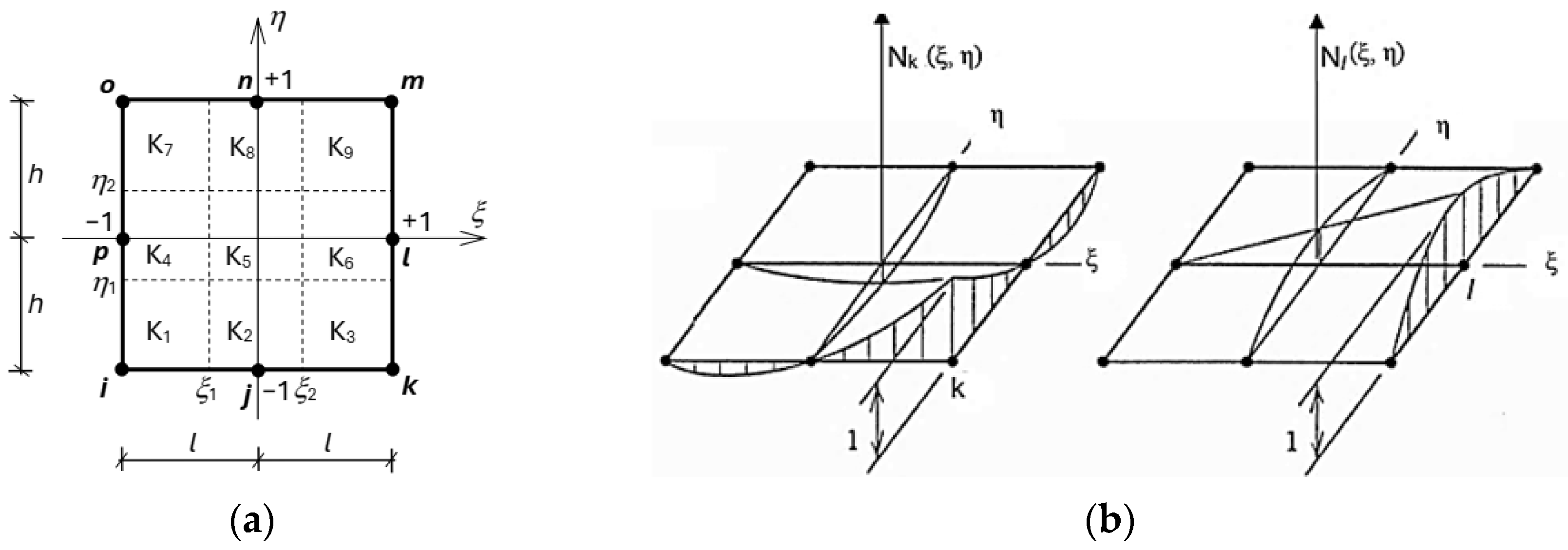
Further development of the method allowed for extension of the concept to two-dimensional elements. The area of the four-node finite element was divided into nine component sub-areas with dimensions defined in natural coordinates ξ and η (see Figure 5a). This allows the insertion of inclusions of any location within the area of the element.
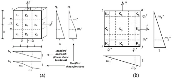
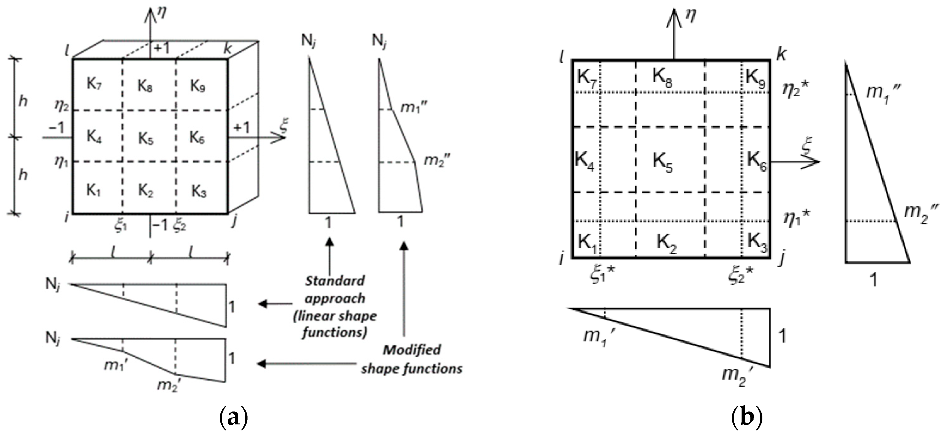
Figure 5.
Definition of multi-area two-dimensional element: (a) broken shape functions; (b) extension of the broken shape functions.
The well-known technique of finite element integration and summation in sub-areas is used. However, this technique with linear shape functions is not effective in the case of significant stiffness differences between the component sub-areas. The problem is solved by using the method of adjusting the shape functions distribution to the changes in the component sub-areas stiffness. The original function for modification of the linear distribution of the shape functions has been developed.
The stiffness matrix of the multi-area finite element (Figure 5) can be described by the expression:
where ti (for i = 1, 2, …, n)—thickness of individual sub-area, and Ωi (for i = 1, 2, …, n)—area of the individual integration sub-area.
In the standard approach, it is assumed that the shape functions do not change and remain linear (Figure 5a). Such an interpretation is justified for small differences in the stiffness of individual sub-areas of the finite element, because the effect of changing the displacement field is not so significant. For greater differences in stiffness, such an approach leads to increasingly large calculation errors and modification of the displacement field inside the finite element is obvious. Modification of the displacement field is in the form of broken shape functions (Figure 5a). For a two-dimensional element, the shape functions are the surface resulting from the components about the ξ and η axes, described by the coefficients m1′, m2′, …, mi′ and m1″, m2″, …, mi″, respectively (Figure 5a).
As a result of such a modification, the shape functions in the form of piecewise broken lines are obtained. The stiffness matrix of the single sub-area is formulated using eight parameters: ξ1, ξ2, η1, η2, m1′, m2′, m1″, m2″.
Similarly to the case of a one-dimensional element [36], the stiffness matrix of a multi-area two-dimensional element is proposed to be determined in an explicit form, which will increase the computational efficiency in relation to numerical integration. Based on expression (6), it should be noted that the matrix of a multi-area element is a sum of the component matrices. The optimal solution is, therefore, to determine the sub-area matrix in a repeatable form. This was obtained by adopting general integration limits in the form of ξ1 to ξ2 for the ξ axis and η1 to η2 for the η axis, and the values of the shape function at the beginning and the end of the sub-area for the ξ axis as m1′, m2′ and for the η axis as m1″, m2″.
Deriving the stiffness matrix of a single component area defined in this way is quite complicated, as it requires the substitution of eight parameters. In order to simplify the final form of the stiffness matrix, the parameters m1′, m2′, m1″, m2″ are made dependent on the integration limits ξ1, ξ2, η1, η2, developing the extension of the integration range. The extension idea of the broken shape functions is illustrated in Figure 5b.
The extension of the integration range changes the boundaries, and the final form of the shape functions again takes the form of linear functions. For example, for a two-dimensional element with nine component areas, where the sub-area K5 has much lower stiffness than the others, extension of the integration range leads to a substitute element with a changed range of sub-areas, which is schematically shown in Figure 5b. The applied method significantly simplifies the final explicit form of the stiffness matrix of the component area and eliminates potential over-stiffening related to the use of broken functions.
It is assumed that the structures analyzed using multi-area elements contain multi-coherent areas and are made of a material that is non-homogeneous. A non-homogeneous material at different points of the area considered has different properties (material characteristics), i.e., it contains various types of defects, inclusions etc. In the case of the material matrix of a two-dimensional multi-area element, the Young’s modulus was divided into one assigned to the horizontal direction E1 and one assigned to the vertical direction E2. For the same purpose, G1 and G2 values were also used. This notation can be described as the identification of the shape functions’ directions. The separation is due to the shape function distribution, separately on the horizontal and vertical directions of the multi-area element.
In this case, the material matrix takes the following form:
where E1—Young’s modulus on the direction of the axis ξ,
E2—Young’s modulus on the direction of the axis η,
G1—shear modulus on the direction of the axis ξ,
G2—shear modulus on the direction of the axis η.
For such assumptions, the stiffness matrix of a single component sub-area is determined from the relationship where two strain matrices are introduced and .
The strain matrices were determined from the standard transformation.
The differential operators take the following form:
After integration of expression (8), the explicit form of the stiffness matrix of a single sub-area in a multi-area element can be written as follows:
where
The symbols which are used to describe the individual matrix elements are as follows:
The form of the stiffness matrix (11) corresponds to the standard two-dimensional element in the explicit notation. This is due to the determination of 10 coefficients of a quite complex structure. It was found that the form of the stiffness matrix is the same, as with the number of multiplication-addition operations, as for the standard element. Thus, it does not increase the computer’s computation time in relation to determining the stiffness matrix of a single finite element. Therefore, the main reason for extending the time of determining the stiffness matrix of the finite element is the fact that it has to be performed as many times as there are sub-areas. For the element divided into nine sub-areas (Figure 5), the time needed to determine a single element matrix automatically increases nine times. From application of FEM analysis, it is known that in standard numerical analyses, the time for determining the value of the element matrices is negligible in relation to the time needed by the solver for the procedure of solving linear equations, which absorbs the majority of the processor’s work.
According to the determined method, the multi-area element could be replaced by a system of connected springs. In Figure 6 and Figure 7, the basic idea of determining the matrix parameters for the direction of horizontal axis ξ and vertical axis η are presented, respectively. Taking into account linear deformations, it is assumed that the equivalent spring system creates a model defined by series-connected springs. Using the determined stiffness parameters k, the values of mi coefficients are calculated [36].
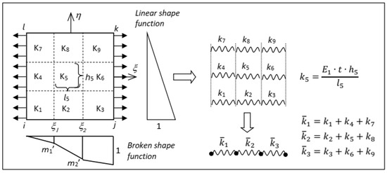
Figure 6.
Model for determining the equivalent integration limits on the direction of the ξ axis.
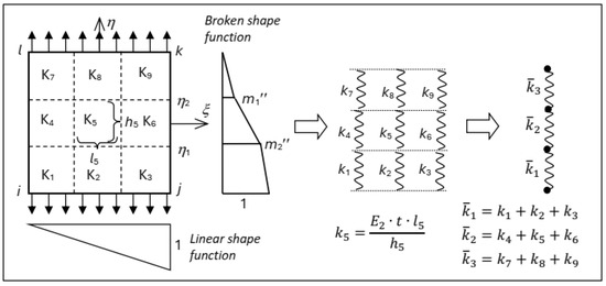
Figure 7.
Model for determining the equivalent integration limits on the direction of the η axis.
Since the shear modulus G changes proportionally to the longitudinal modulus of elasticity E, the same models are used for the shear deformations in the element. This allows the use of the same coefficients for the component sub-areas. This greatly simplifies the process of determining the stiffness matrix of the entire element.
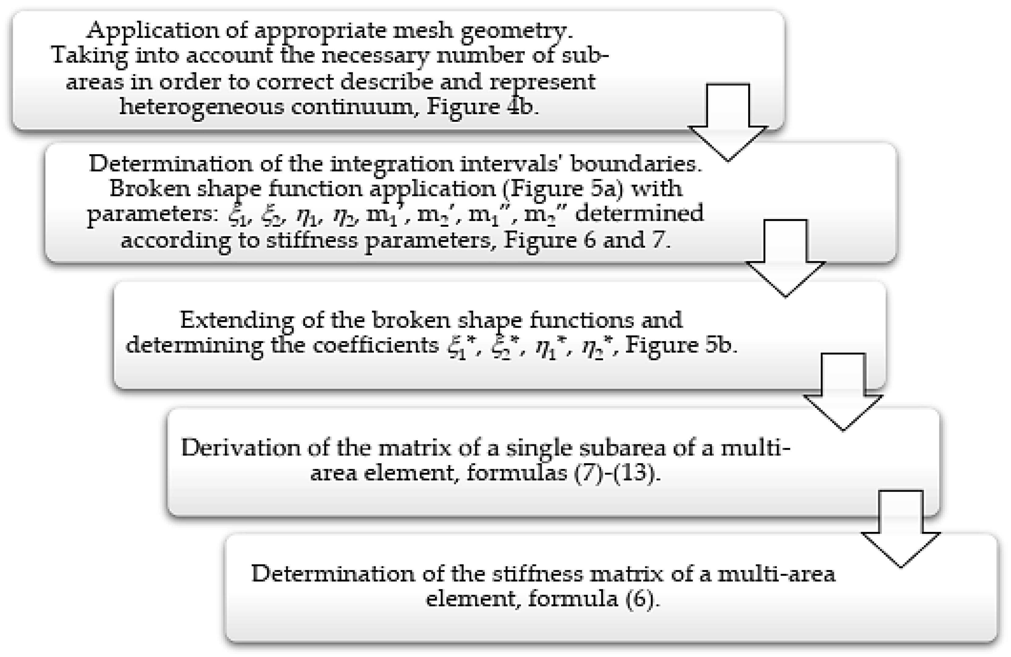
The presented process of deriving the stiffness matrix of the multi-area element has been described in detail. To enhance comprehension, an explanatory diagram of the consecutive steps of the procedure has been developed and is shown in Figure 8.
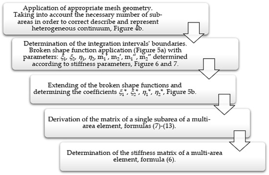
Figure 8.
Main stages of determining the stiffness matrix of a multi-area element.
2.3. Eight-Node Elements
Based on the four-node element, an eight-node element was also developed (see Figure 9a). Examples of the shape functions used are shown in Figure 9b.
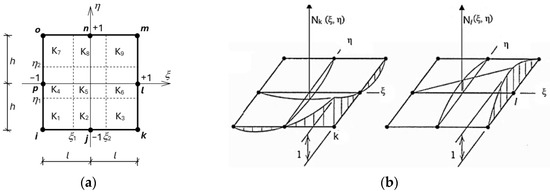
Figure 9.
Eight-node element: (a) division in sub-areas; (b) exemplary shape functions.
In the case of the eight-node elements, broken shape functions coefficients were determined using the same assumptions as in the four-node elements. The main difference is the application of the shape functions that are typical for eight-node elements:
3. Numerical Tests
3.1. Heterogeneous Structure Composed of Square Elements 20 × 20 cm Containing Symmetrically Increasing Square Inclusions
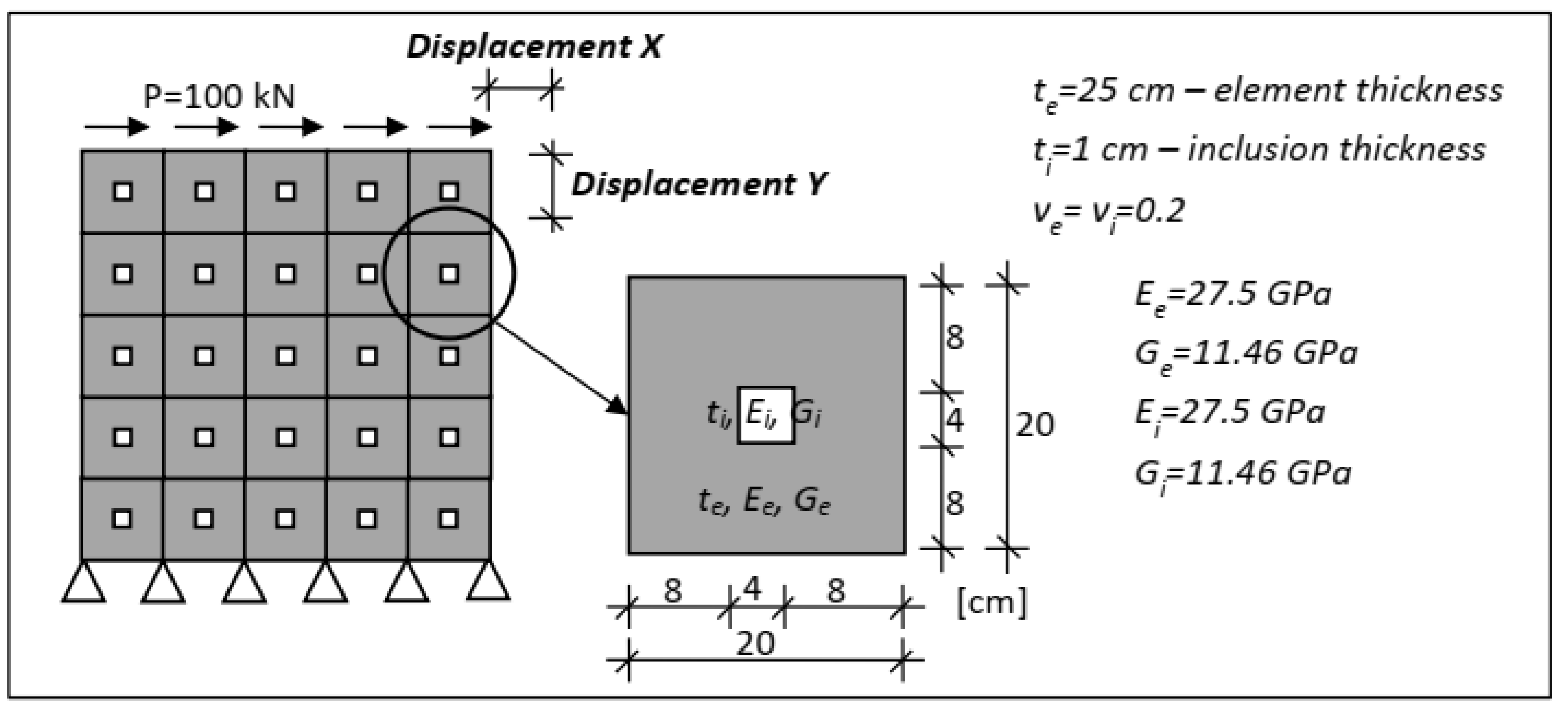
The proposed method and its assumptions were verified using the example of displacements calculations of a structure consisting of elements in the plane state of stress (Figure 10). The tests presented are analogous to the elements or the parts of the structures made of non-homogeneous materials, containing areas with variable stiffness characteristics. The structure consists of square elements 20 × 20 cm with a thickness of 25 cm containing centrally located inclusions in the form of a weakening cross-section with a thickness of 1 cm. The centrally located inclusions have the following sizes: 4 × 4 cm, 8 × 8 cm, 12 × 12 cm, 16 × 16 cm. In all variants, the total load was 100 kN in the form of a uniformly distributed load applied to the edge of the structure.

Figure 10.
Model for numerical test no. 1 with multi-area elements.
In order to demonstrate the necessity of modifying the displacement field in the case of structures containing areas of different stiffness, calculations were performed using multi-area elements and elements integrated in sub-areas with linear shape functions. Numerical calculations using multi-area elements and elements integrated in sub-areas with linear shape functions were performed using our own developed calculation formulas with the computer programs Maxima [37] and Orcan [38].
Reference values were obtained from standard, analytical FEM calculations performed and checked using the computer programs Maxima [37] and Orcan [38]. In the case of FEM calculations, a typical discretization was used, according to which nine separate elements were used instead of one multi-area element. This resulted in significant differences in the number of finite elements. The FEM model consisted of a total of 225 elements, while the same model using multi-area elements consisted of 25 finite elements.
To summarize, in test no. 1, the displacement analysis was performed for three computational models:
- model with multi-area four-node elements, i.e., modified according to the presented method,
- model with four-node elements integrated in sub-areas with linear shape functions, i.e., without modification of the shape functions,
- reference model with standard discretization.
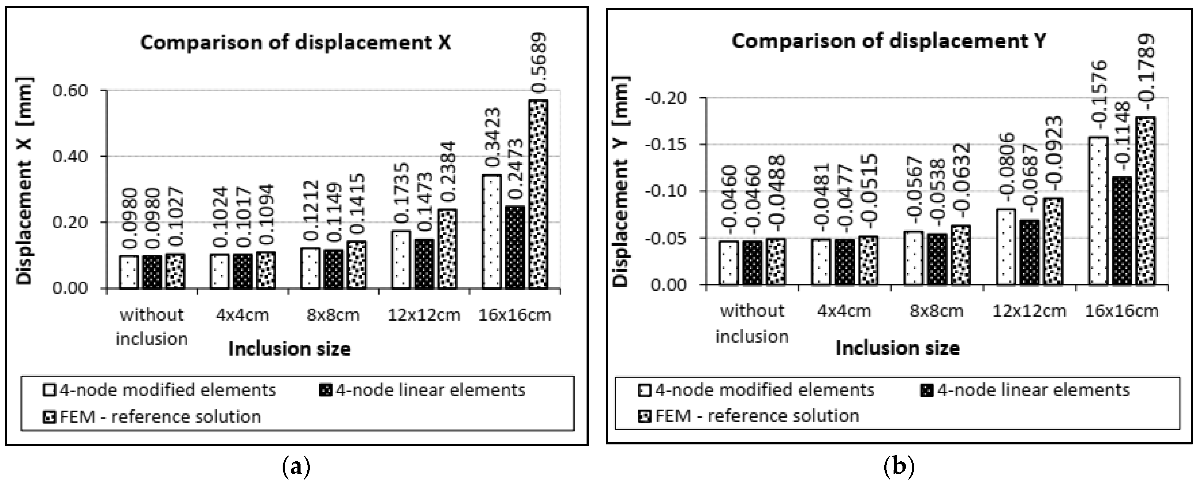
A comparison of the obtained displacement values is presented in Figure 11. The displacements are presented according to the X- and Y-directions indicated in Figure 10.
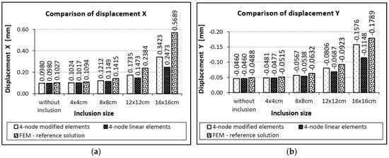
Figure 11.
Displacement values for model of heterogeneous structure: (a) on the X-direction; (b) on the Y-direction.
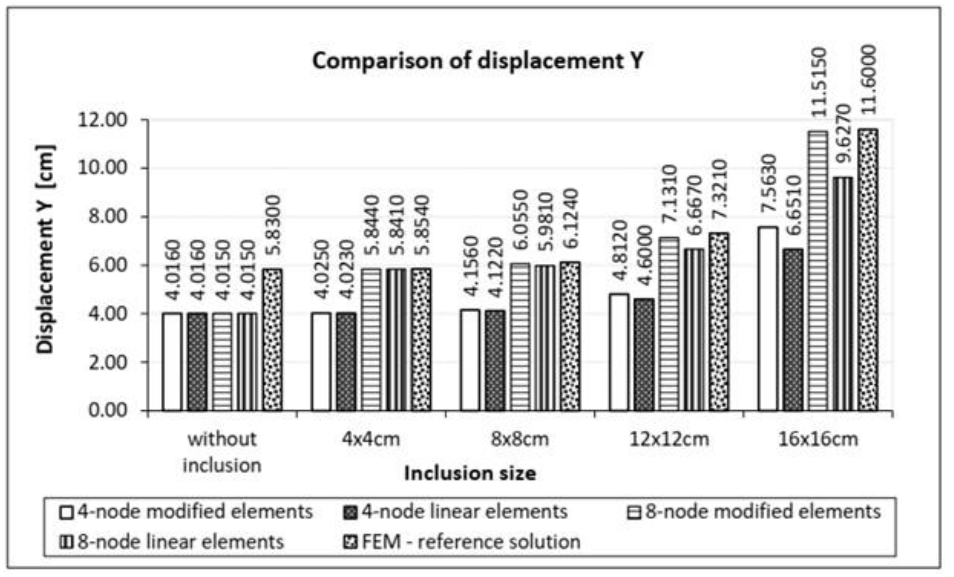
3.2. Cantilever Beam Composed of 20 × 20 cm Square Elements Containing Symmetrically Increasing Square Inclusions
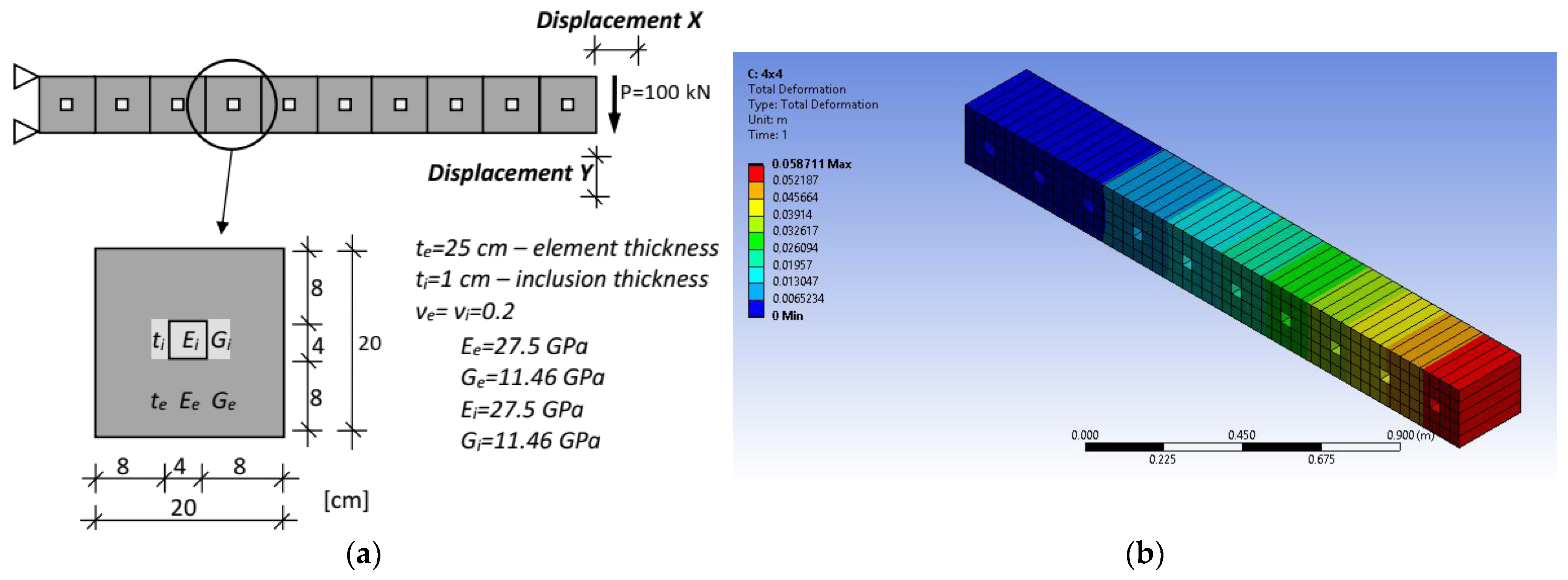
The presented method was also verified using the example of a cantilever beam consisting of elements in a plane state of stress. The parameters of the calculation model are presented in Figure 12a. As in the previous test no.1, this example is also analogous to elements or parts of structures made of heterogeneous materials, containing cross-sectional defects or damages. The 20 × 20 cm elements with a thickness of 25 cm contain centrally located inclusions in the form of a cross-section weakening with a thickness of 1 cm. Calculations were performed for the following sizes of inclusions: 4 × 4 cm, 8 × 8 cm, 12 × 12 cm, 16 × 16 cm. In all variants, the total load was 100 kN. Numerical calculations using modified elements were carried out using the Maxima [37] and Orcan [38] programs, where own developed calculation formulas were implemented. For the reference solution, numerical calculations were performed using the Ansys program [39] (see Figure 12b).

Figure 12.
Model for the numerical test no. 2: (a) model geometry and parameters; (b) calculation model in program Ansys.
For test no. 2, calculations were performed for the following variants, where different types of finite elements were used:
- four-node elements with modification according to the presented method,
- four-node elements without modification of the shape functions,
- eight-node elements with modification according to the presented method,
- eight-node elements without modification of the shape functions,
- reference model with standard discretization.

Figure 13.
Results of the displacement on the Y-direction.
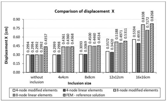
Figure 14.
Results of the displacement on the X-direction.
4. Discussion
According to the results obtained from numerical test no.1, it can be confirmed that the application of modified finite elements in the calculations of structures with variable stiffness and geometric parameters provides results that are consistent or very close to the expected solution. In test no. 2, both four-node and eight-node modified elements provide more accurate results than those obtained using elements integrated in sub-areas without modification of the shape function distribution. Eight-node elements are characterized by a greater increase in solution efficiency compared to four-node elements. In the variant without inclusion, the results differ because the reference solution was determined for the discretization model with more elements.
Due to determination of the stiffness matrix in an explicit form, the influence of stiffness changes in individual sub-areas within a single element is taken into account. It is possible to more clearly control the insertion of potential weaknesses and defects in the element. Determining the repeatable form of the stiffness matrix of a single sub-area significantly simplifies this process.
The presented computational tests and results demonstrated that the use of elements integrated in sub-areas in a standard way with linear shape functions leads to incorrect results. The approach is acceptable only with negligible differences between the stiffnesses of the sub-areas. Strain field modification inside the element is necessary in the case of significant differences in the material parameters. The greater the difference between the sub-areas’ stiffness, the greater the computational error. Therefore, strain field modification using the broken shape functions was proposed. The use of modified finite elements makes it possible to obtain results that are close to the expected solution even where there are significant differences in the stiffness of the component sub-areas. The presented method can provide results that can be used to control the serviceability limit states and prevent potential failure of structure.
5. Conclusions
An original matrix method for analyzing heterogeneous structures containing defects and damages, i.e., areas with different geometric and material parameters, was developed and used in the FEM. The method reduces the number of unknowns by several times compared to standard FEM solutions and reduces the time and costs of numerical analyses. Explicit stiffness matrices for two-dimensional modified four-node and eight-node elements were developed.
The usefulness of the developed special multi-area elements in the analysis of periodic structures containing weaknesses, material defects, and damages was confirmed. This applies especially when it is necessary to analyze the influence of regularly distributed areas of variable stiffness on the displacements of the entire structure. The need to control the calculations conducted was emphasized, especially in terms of the assumptions and simplifications of the calculation models. The developed method provides a quick and undemanding way to verify the number of potential damages that will cause the structure to exceed its limit state.
Author Contributions
Conceptualization, M.M. and T.C.; methodology, M.M. and T.C.; software, T.C.; validation, M.M.; formal analysis, M.M.; investigation, M.M.; resources, T.C.; data curation, M.M; writing—original draft preparation, M.M.; writing—review and editing, M.M.; visualization, M.M.; supervision, T.C.; project administration, M.M.; funding acquisition, T.C. All authors have read and agreed to the published version of the manuscript.
Funding
The research was carried out within the scope of works no. WZ/WB-IIL/4/2023 of the Bialystok University of Technology and was financed from the resources for science of the Ministry of Science and Higher Education of Poland.
Institutional Review Board Statement
Not applicable.
Informed Consent Statement
Not applicable.
Data Availability Statement
Some or all data, models, or code that support the findings of this study are available from the corresponding author upon reasonable request.
Conflicts of Interest
The authors declare no conflicts of interest.
References
- Stachowski, A. Porous Materials as Future Application in Constructions. Kompozyty (Composites) 2001, 1, 224–227. [Google Scholar]
- Adamczyk, M.; Niżnik-Harańczyk, B.; Pogorzałek, J. The Effect of Melting Technologyof Steel with Addition of 3÷5% Al on the Type and Morphology of Non-Metallic Inclusions. Pr. Inst. Metal. Żelaza 2016, 68, 24–32. [Google Scholar]
- Addessi, D.; Mastrandrea, A.; Sacco, E. An Equilibrated Macro-Element for Nonlinear Analysis of Masonry Structures. Eng. Struct. 2014, 70, 82–93. [Google Scholar] [CrossRef]
- Caliò, I.; Pantò, B. A Macro-Element Modelling Approach of Infilled Frame Structures. Comput. Struct. 2014, 143, 91–107. [Google Scholar] [CrossRef]
- Liao, A.; Li, Y. A Super Element Model for Failure Analysis of Masonry Buildings under Lateral In-Plane Loading. Eng. Fail. Anal. 2025, 168, 109088. [Google Scholar] [CrossRef]
- Drougkas, A. Macro-Modelling of Orthotropic Damage in Masonry: Combining Micro-Mechanics and Continuum FE Analysis. Eng. Fail. Anal. 2022, 141, 106704. [Google Scholar] [CrossRef]
- Gaetano, D.; Greco, F.; Leonetti, L.; Lonetti, P.; Pascuzzo, A.; Ronchei, C. An Interface-Based Detailed Micro-Model for the Failure Simulation of Masonry Structures. Eng. Fail. Anal. 2022, 142, 106753. [Google Scholar] [CrossRef]
- Benkhechiba, A.E.; Guesmia, M.; Hachi, B.E.; Hachi, D.; Moussaoui, M. Contribution to the Modelling and Homogenization of 3D Structures in the Presence of Flaws by XFEM. Eng. Fail. Anal. 2020, 107, 104219. [Google Scholar] [CrossRef]
- Haghani, M.; Neya, B.N.; Ahmadi, M.T.; Amiri, J.V. A New Numerical Approach in the Seismic Failure Analysis of Concrete Gravity Dams Using Extended Finite Element Method. Eng. Fail. Anal. 2022, 132, 105835. [Google Scholar] [CrossRef]
- Kotšmíd, S.; Beňo, P. A Low Computational Cost Optimization Procedure for Axial Load Carrying Capacity of the Multi-Beam Structure. Eng. Fail. Anal. 2023, 143, 106922. [Google Scholar] [CrossRef]
- Cong, T.; Wang, J.; He, J.; Liu, Y.; Chen, Y.; Liu, F.; Li, L. Microstructure Evolution and Fatigue Crack Initiation Life Prediction of Actual Failed Bearings under GRCF Conditions. Eng. Fail. Anal. 2025, 169, 109148. [Google Scholar] [CrossRef]
- Ma, A.; Zhang, Y.; Dong, L.; Yan, H.; Fang, F.; Li, Z. Damage and Fracture Analyses of Wire with Off-Center Inclusion on Multi-Pass Drawing under Different Back Tensions. Eng. Fail. Anal. 2022, 139, 106512. [Google Scholar] [CrossRef]
- Dhanya, M.S.; Ranjith, R.; Manwatkar, S.K.; Kumar Gupta, R.; Narayana Murty, S.V.S. Metallurgical Investigation on Failure of Plain Carbon Steel Piston Rod Used in Hydraulic Jack: Role of Inclusions and Surface Roughness. Eng. Fail. Anal. 2023, 150, 107346. [Google Scholar] [CrossRef]
- Fan, Y.; Shuai, Y.; Shuai, J.; Zhang, T.; Zhang, Y.; Shi, L.; Shan, K. The Effect of Pipeline Root Weld Microstructure on Crack Growth Behaviour. Eng. Fail. Anal. 2024, 161, 108265. [Google Scholar] [CrossRef]
- Eshelby, J.D. The Determination of the Elastic Field of an Ellipsoidal Inclusion, and Related Problems The Determination of the Elastic Field of an Elli p Soidal Inclusion, and Related p Roblems. Proc. R. Soc. Lond. A Math. Phys. Sci. 1957, 241, 376–396. [Google Scholar] [CrossRef]
- Eshelby, J.D. The Elastic Field Outside an Ellipsoidal Inclusion. Proc. R. Soc. Lond. A Math. Phys. Sci. 1959, 252, 561–569. [Google Scholar] [CrossRef]
- Mazzucco, G.; Pomaro, B.; Salomoni, V.A.; Majorana, C.E. Numerical Modelling of Ellipsoidal Inclusions. Constr. Build. Mater. 2018, 167, 317–324. [Google Scholar] [CrossRef]
- Nguyen, S.-T.; To, Q.-D.; Vu, M.-N.; Nguyen, T.-D. Viscoelastic Properties of Heterogeneous Materials: The Case of Periodic Media Containing Cuboidal Inclusions. Compos. Struct. 2016, 157, 275–284. [Google Scholar] [CrossRef]
- Zhou, K.; Hoh, H.J.; Wang, X.; Keer, L.M.; Pang, J.H.L.; Song, B.; Wang, Q.J. A Review of Recent Works on Inclusions. Mech. Mater. 2013, 60, 144–158. [Google Scholar] [CrossRef]
- Pan, C.; Yu, Q. Inclusion Problem of a Two-Dimensional Finite Domain: The Shape Effect of Matrix. Mech. Mater. 2014, 77, 86–97. [Google Scholar] [CrossRef]
- Yvonnet, J.; Gonzalez, D.; He, Q.-C. Numerically Explicit Potentials for the Homogenization of Nonlinear Elastic Heterogeneous Materials. Comput. Methods Appl. Mech. Eng. 2009, 198, 2723–2737. [Google Scholar] [CrossRef]
- Cecot, W.; Oleksy, M. High Order FEM for Multigrid Homogenization. Comput. Math. Appl. 2015, 70, 1391–1400. [Google Scholar] [CrossRef]
- Ho, S.-P.; Yeh, Y.-L. The Use of 2D Enriched Elements with Bubble Functions for Finite Element Analysis. Comput. Struct. 2006, 84, 2081–2091. [Google Scholar] [CrossRef]
- Matsui, K.; Terada, K.; Yuge, K. Two-Scale Finite Element Analysis of Heterogeneous Solids with Periodic Microstructures. Comput. Struct. 2004, 82, 593–606. [Google Scholar] [CrossRef]
- Zhang, H.W.; Liu, Y.; Zhang, S.; Tao, J.; Wu, J.K.; Chen, B.S. Extended Multiscale Finite Element Method: Its Basis and Applications for Mechanical Analysis of Heterogeneous Materials. Comput. Mech. 2014, 53, 659–685. [Google Scholar] [CrossRef]
- Xing, Y.F.; Yang, Y. An Eigenelement Method of Periodical Composite Structures. Compos. Struct. 2011, 93, 502–512. [Google Scholar] [CrossRef]
- Xing, Y.F.; Du, C.Y. An Improved Multiscale Eigenelement Method of Periodical Composite Structures. Compos. Struct. 2014, 118, 200–207. [Google Scholar] [CrossRef]
- Xing, Y.; Gao, Y. Multiscale Eigenelement Method for Periodical Composites: A Review. Chin. J. Aeronaut. 2019, 32, 104–113. [Google Scholar] [CrossRef]
- Gao, Y.; Xing, Y.; Huang, Z.; Li, M.; Yang, Y. An Assessment of Multiscale Asymptotic Expansion Method for Linear Static Problems of Periodic Composite Structures. Eur. J. Mech. A/Solids 2020, 81, 103951. [Google Scholar] [CrossRef]
- Liu, H.; Sun, X.; Xu, Y.; Chu, X. A Hierarchical Multilevel Finite Element Method for Mechanical Analyses of Periodical Composite Structures. Compos. Struct. 2015, 131, 115–127. [Google Scholar] [CrossRef]
- Kim, S.; Lee, P.S. A New Enriched 4-Node 2D Solid Finite Element Free from the Linear Dependence Problem. Comput. Struct. 2018, 202, 25–43. [Google Scholar] [CrossRef]
- Ahmad, B.; Alsaedi, A.; Brezzi, F.; Marini, L.D.; Russo, A. Equivalent Projectors for Virtual Element Methods. Comput. Math. Appl. 2013, 66, 376–391. [Google Scholar] [CrossRef]
- Brezzi, F.; Marini, L.D. Virtual Element Methods for Plate Bending Problems. Comput. Methods Appl. Mech. Eng. 2013, 253, 455–462. [Google Scholar] [CrossRef]
- Desiderio, L.; Falletta, S.; Ferrari, M.; Scuderi, L. CVEM-BEM Coupling with Decoupled Orders for 2D Exterior Poisson Problems. J. Sci. Comput. 2022, 92, 96. [Google Scholar] [CrossRef]
- Desiderio, L.; Falletta, S.; Scuderi, L. A Virtual Element Method Coupled with a Boundary Integral Non Reflecting Condition for 2D Exterior Helmholtz Problems. Comput. Math. Appl. 2021, 84, 296–313. [Google Scholar] [CrossRef]
- Chyży, T.; Mackiewicz, M. Special Finite Elements with Adaptive Strain Field on the Example of One-Dimensional Elements. Appl. Sci. 2021, 11, 609. [Google Scholar] [CrossRef]
- Available online: https://maxima.sourceforge.net (accessed on 1 March 2025).
- Chyży, T.; Mackiewicz, M.; Matulewicz, S. Modern Graphic Language for Description of Building Structures, Orcan Ver. 0.91. 2014. (In Polish). Available online: http://orcanfree.pl/Instrukcja%20ORCAN%20v.4.pdf (accessed on 1 March 2025).
- ANSYS Inc. Ansys R2; Computer Program; Ansys: Canonsburg, PA, USA, 2022. [Google Scholar]


Disclaimer/Publisher’s Note: The statements, opinions and data contained in all publications are solely those of the individual author(s) and contributor(s) and not of MDPI and/or the editor(s). MDPI and/or the editor(s) disclaim responsibility for any injury to people or property resulting from any ideas, methods, instructions or products referred to in the content. |
© 2025 by the authors. Licensee MDPI, Basel, Switzerland. This article is an open access article distributed under the terms and conditions of the Creative Commons Attribution (CC BY) license (https://creativecommons.org/licenses/by/4.0/).