
Automated Residential Bubble Diagram Generation Based on Dual-Branch Graph Neural Network and Variational Encoding


Abstract
1. Introduction
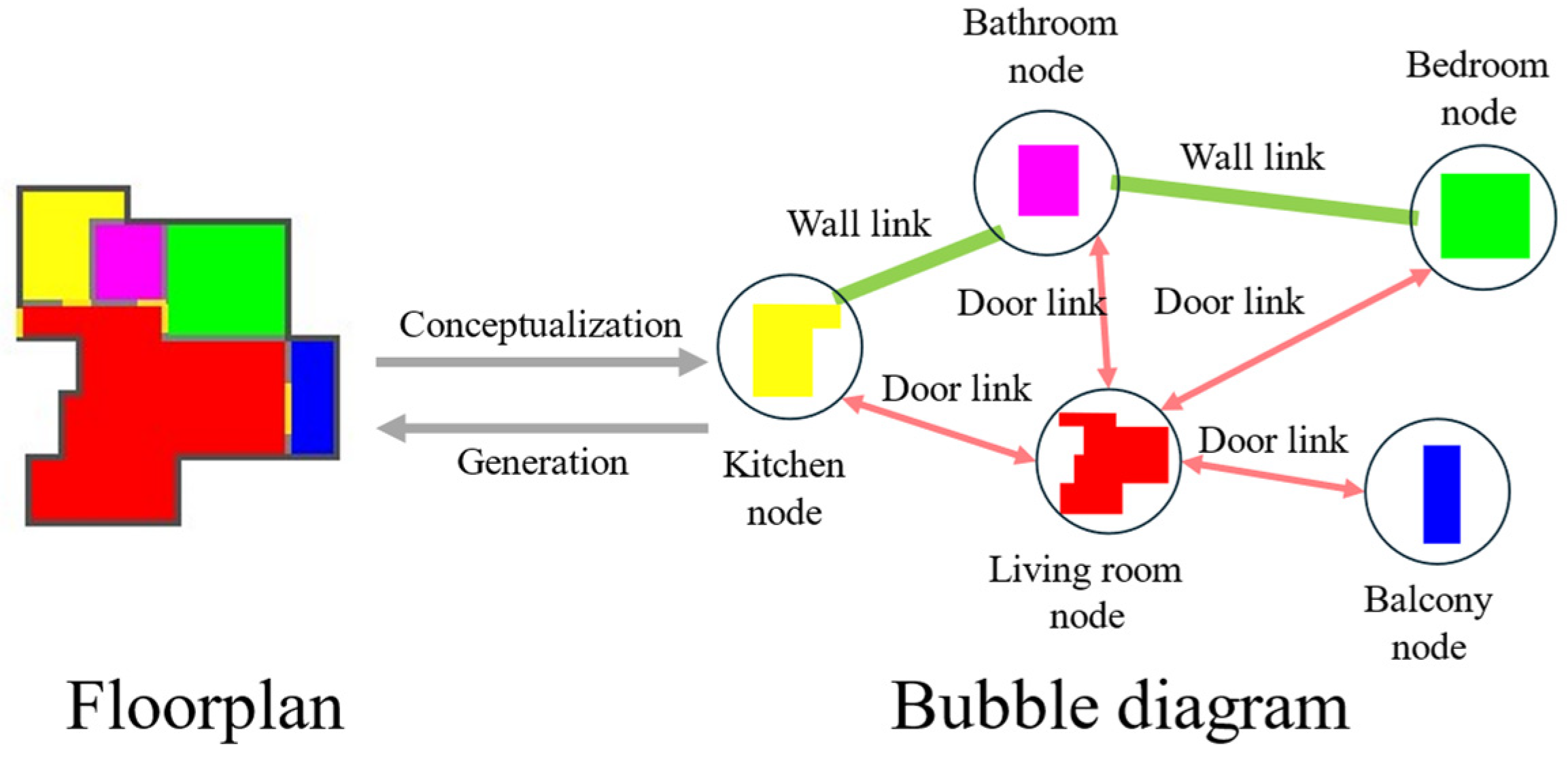
2. Preliminary
3. Methodology
3.1. Overall Framework
3.2. Dual-Branch Graph Neural Network for Bubble Diagram Link Prediction
3.2.1. Graph Normalization
3.2.2. Decentralized Node Subgraph Sampling and Centralized Node Subgraph Sampling
3.2.3. Link Prediction Decoder
3.3. Variational Encoding for Diverse Bubble Diagram Generation
3.4. Multi-Task Loss Functions
3.5. Evaluation Metrics
4. Experiments
4.1. Bubble Diagram Dataset Establishment
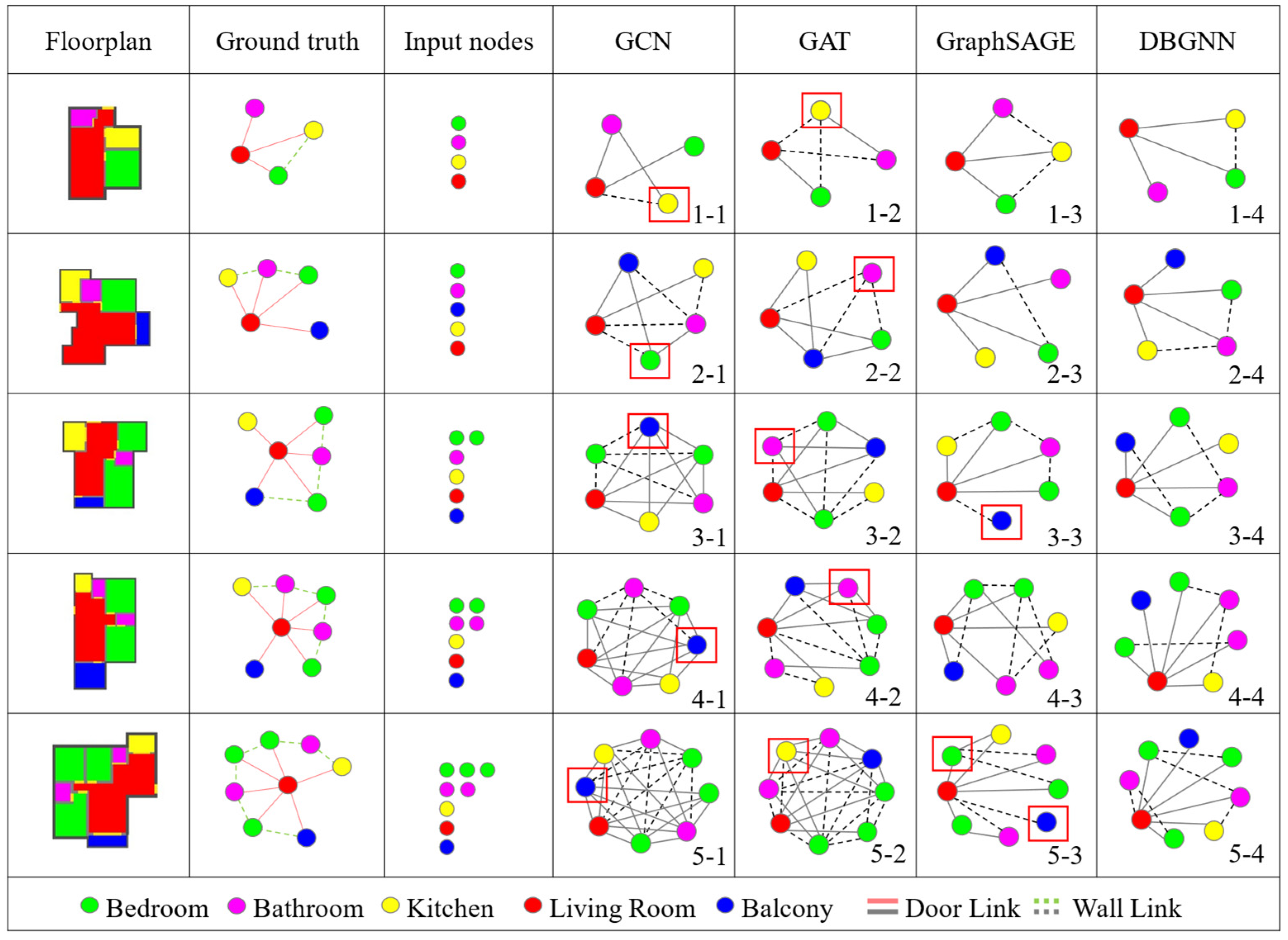
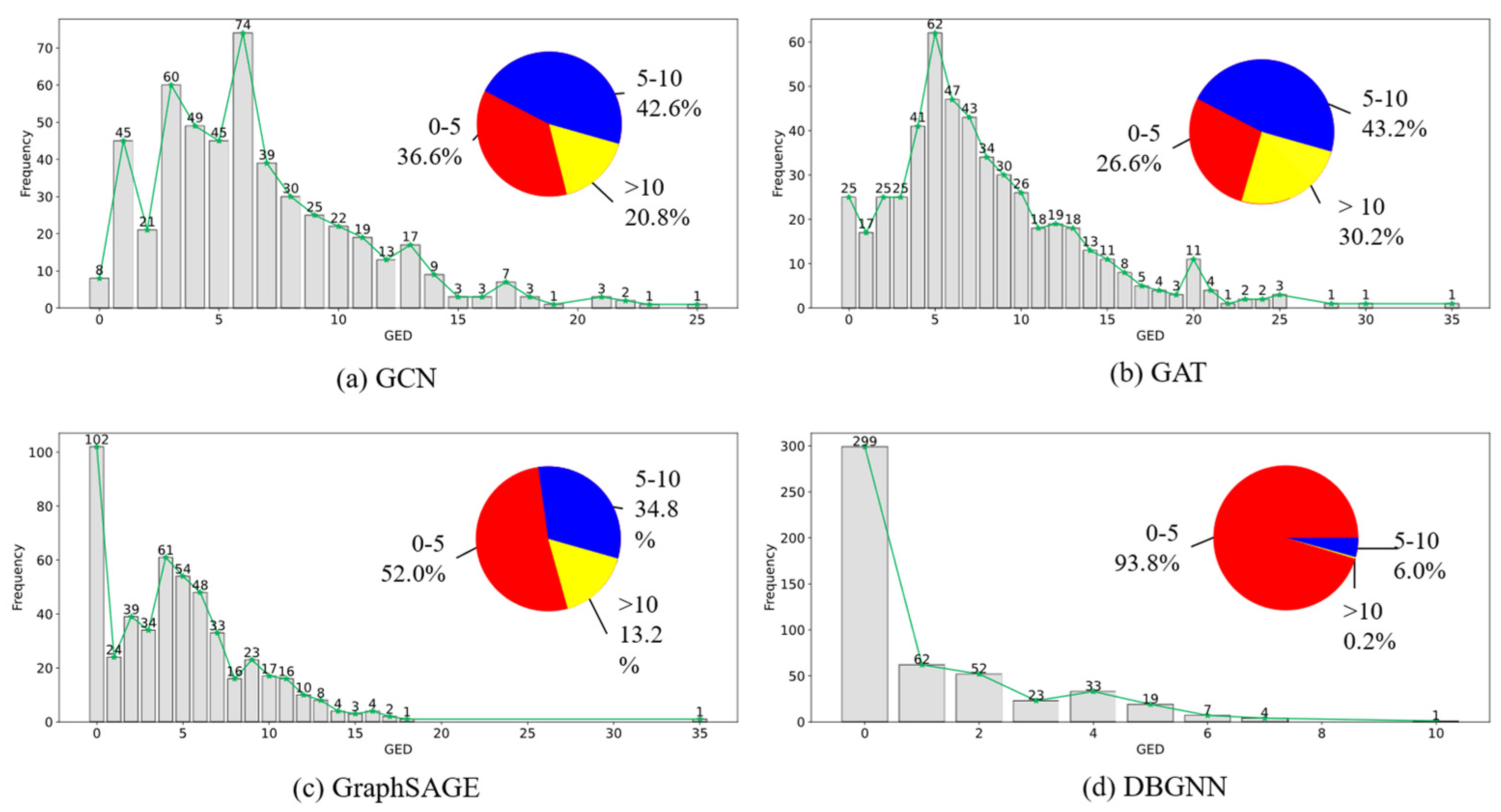
4.2. Model Training and Performance Comparison
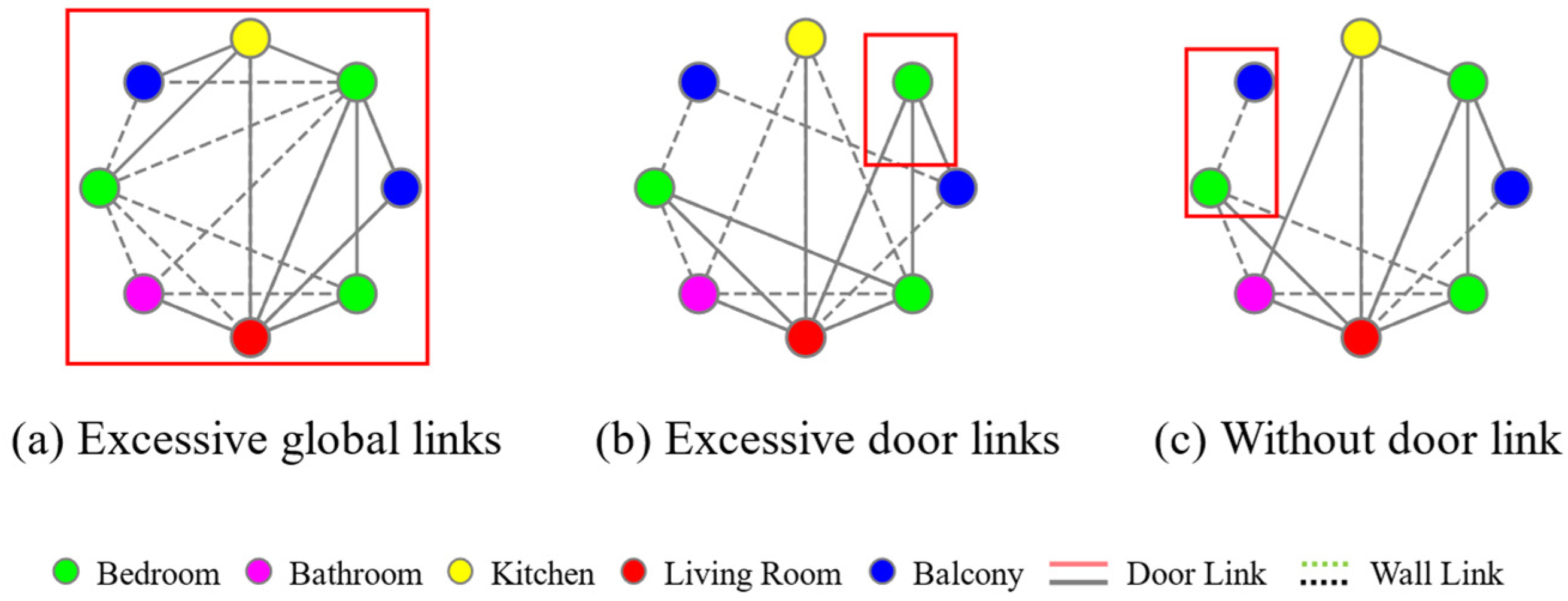
4.3. Ablation Experiment
4.4. Diverse Bubble Diagrams Generation
4.5. Diversity Evaluation
4.6. Usability Evaluation
4.7. Time Efficiency Study
5. Discussion
5.1. Application
5.2. Limitations
6. Conclusions and Future Works
Author Contributions
Funding
Institutional Review Board Statement
Informed Consent Statement
Data Availability Statement
Conflicts of Interest
References
- Weber, R.E.; Mueller, C.; Reinhart, C. Automated floorplan generation in architectural design: A review of methods and applications. Autom. Constr. 2022, 140, 104385. [Google Scholar] [CrossRef]
- Luo, Z.; Huang, W. Floorplangan: Vector residential floorplan adversarial generation. Autom. Constr. 2022, 142, 104470. [Google Scholar] [CrossRef]
- Kutzias, D.; von Mammen, S. Recent advances in procedural generation of buildings: From diversity to integration. IEEE Trans. Games 2023, 16, 16–35. [Google Scholar] [CrossRef]
- Aalaei, M.; Saadi, M.; Rahbar, M.; Ekhlassi, A. Architectural layout generation using a graph-constrained conditional generative adversarial network (gan). Autom. Constr. 2023, 155, 105053. [Google Scholar] [CrossRef]
- Tang, H.; Shao, L.; Sebe, N.; Van Gool, L. Graph transformer gans with graph masked modeling for architectural layout generation. IEEE Trans. Pattern Anal. Mach. Intell. 2024, 46, 4298–4313. [Google Scholar] [CrossRef]
- Zheng, Z.; Petzold, F. Neural-guided room layout generation with bubble diagram constraints. Autom. Constr. 2023, 154, 104962. [Google Scholar] [CrossRef]
- Xiang, J.; Hou, B.; Chen, X.; Qi, H.; Feng, L.; Liu, J.; Li, X. House Layout Generation via Diffusion Model with Relative Room Area Ranking. In Proceedings of the 2024 International Joint Conference on Neural Networks (IJCNN), Yokohama, Japan, 30 June–5 July 2024; pp. 1–8. [Google Scholar]
- Sun, J.; Wu, W.; Liu, L.; Min, W.; Zhang, G.; Zheng, L. Wallplan: Synthesizing floorplans by learning to generate wall graphs. ACM Trans. Graph. (TOG) 2022, 41, 1–14. [Google Scholar] [CrossRef]
- Nauata, N.; Chang, K.-H.; Cheng, C.-Y.; Mori, G.; Furukawa, Y. House-Gan: Relational Generative Adversarial Networks for Graph-Constrained House Layout Generation. In Computer Vision–ECCV 2020: 16th European Conference, Glasgow, UK, 23–28 August 2020; Proceedings, Part I 16; Springer: Berlin/Heidelberg, Germany, 2020; pp. 162–177. [Google Scholar]
- Shabani, M.A.; Hosseini, S.; Furukawa, Y. Housediffusion: Vector floorplan generation via a diffusion model with discrete and continuous denoising. arXiv 2022, arXiv:2211.13287. [Google Scholar]
- Hu, R.; Huang, Z.; Tang, Y.; Van Kaick, O.; Zhang, H.; Huang, H. Graph2plan: Learning floorplan generation from layout graphs. ACM Trans. Graph. (TOG) 2020, 39, 118:1–118:14. [Google Scholar] [CrossRef]
- He, F.; Huang, Y.; Wang, H. iplan: Interactive and Procedural Layout Planning. In Proceedings of the IEEE/CVF Conference on Computer Vision and Pattern Recognition, New Orleans, LA, USA, 18–24 June 2022; pp. 7793–7802. [Google Scholar]
- Nauata, N.; Hosseini, S.; Chang, K.-H.; Chu, H.; Cheng, C.-Y.; Furukawa, Y. House-Gan++: Generative Adversarial Layout Refinement Network Towards Intelligent Computational Agent for Professional Architects. In Proceedings of the IEEE/CVF Conference on Computer Vision and Pattern Recognition, Nashville, TN, USA, 20–25 June 2021; pp. 13632–13641. [Google Scholar]
- Zhao, P.; Liao, W.; Huang, Y.; Lu, X. Intelligent beam layout design for frame structure based on graph neural networks. J. Build. Eng. 2023, 63, 105499. [Google Scholar] [CrossRef]
- Li, K.; Gan, V.J.L.; Li, M.; Gao, M.Y.; Tiong, R.L.K.; Yang, Y. Automated generative design and prefabrication of precast buildings using integrated bim and graph convolutional neural network. Dev. Built Environ. 2024, 18, 100418. [Google Scholar] [CrossRef]
- Paudel, A.; Dhakal, R.; Bhattarai, S. Room classification on floor plan graphs using graph neural networks. arXiv 2021, arXiv:2108.05947. [Google Scholar]
- Wang, Z.; Sacks, R.; Yeung, T. Exploring graph neural networks for semantic enrichment: Room type classification. Autom. Constr. 2022, 134, 104039. [Google Scholar] [CrossRef]
- Zhou, J.; Cui, G.; Hu, S.; Zhang, Z.; Yang, C.; Liu, Z.; Wang, L.; Li, C.; Sun, M. Graph neural networks: A review of methods and applications. AI Open 2020, 1, 57–81. [Google Scholar] [CrossRef]
- Li, X.; Sun, L.; Ling, M.; Peng, Y. A survey of graph neural network based recommendation in social networks. Neurocomputing 2023, 549, 126441. [Google Scholar] [CrossRef]
- Bongini, P.; Bianchini, M.; Scarselli, F. Molecular generative graph neural networks for drug discovery. Neurocomputing 2021, 450, 242–252. [Google Scholar] [CrossRef]
- Fan, W.; Ma, Y.; Li, Q.; Wang, J.; Cai, G.; Tang, J.; Yin, D. A graph neural network framework for social recommendations. IEEE Trans. Knowl. Data Eng. 2020, 34, 2033–2047. [Google Scholar] [CrossRef]
- Hao, Z.; Lu, C.; Huang, Z.; Wang, H.; Hu, Z.; Liu, Q.; Chen, E.; Lee, C. Asgn: An Active Semi-Supervised Graph Neural Network for Molecular Property Prediction. In Proceedings of the 26th ACM SIGKDD International Conference on Knowledge Discovery Data Mining, Virtual Event, 6–10 July 2020; pp. 731–752. [Google Scholar]
- Zhao, P.; Liao, W.; Huang, Y.; Lu, X. Intelligent design of shear wall layout based on graph neural networks. Adv. Eng. Inform. 2023, 55, 101886. [Google Scholar] [CrossRef]
- Zou, D.; Hu, Z.; Wang, Y.; Jiang, S.; Sun, Y.; Gu, Q. Layer-dependent importance sampling for training deep and large graph convolutional networks. Adv. Neural Inf. Process. Syst. 2019, 32, 11249–11259. [Google Scholar]
- Ying, R.; He, R.; Chen, K.; Eksombatchai, P.; Hamilton, W.L.; Leskovec, J. Graph Convolutional Neural Networks for Web-Scale Recommender Systems. In Proceedings of the 24th ACM SIGKDD International Conference on Knowledge Discovery Data Mining, London, UK, 19–23 August 2018; pp. 974–983. [Google Scholar]
- Hamilton, W.; Ying, Z.; Leskovec, J. Inductive representation learning on large graphs. Adv. Neural Inf. Process. Syst. 2017, 30. [Google Scholar]
- Emmons, P. Embodying networks: Bubble diagrams and the image of modern organicism. J. Archit. 2006, 11, 441–461. [Google Scholar] [CrossRef]
- Hendrycks, D.; Gimpel, K. Gaussian error linear units (gelus). arXiv 2016, arXiv:1606.08415. [Google Scholar]
- He, K.; Zhang, X.; Ren, S.; Sun, J. Deep Residual Learning for Image Recognition. In Proceedings of the IEEE Conference on Computer Vision and Pattern Recognition, Las Vegas, NV, USA, 27–30 June 2016; pp. 770–778. [Google Scholar]
- Han, K.; Wang, Y.; Chen, H.; Chen, X.; Guo, J.; Liu, Z.; Tang, Y.; Xiao, A.; Xu, C.; Xu, Y.; et al. A survey on vision transformer. IEEE Trans. Pattern Anal. Mach. Intell. 2022, 45, 87–110. [Google Scholar] [CrossRef]
- Yu, W.; Luo, M.; Zhou, P.; Si, C.; Zhou, Y.; Wang, X.; Feng, J.; Yan, S. Metaformer is Actually What You Need for Vision. In Proceedings of the IEEE/CVF Conference on Computer Vision and Pattern Recognition, New Orleans, LA, USA, 18–24 June 2022; pp. 10819–10829. [Google Scholar]
- Chen, Y.; Tang, X.; Qi, X.; Li, C.-G.; Xiao, R. Learning graph normalization for graph neural networks. Neurocomputing 2022, 493, 613–625. [Google Scholar] [CrossRef]
- Yenew, A.B.; Assefa, B.G.; Belay, E.G. Housegandi: A hybrid approach to strike a balance of sampling time and diversity in floorplan generation. IEEE Access 2024, 125235–125252. [Google Scholar] [CrossRef]
- Kipf, T.N.; Welling, M. Variational graph auto-encoders. arXiv 2016, arXiv:1611.07308. [Google Scholar]
- Abu-Aisheh, Z.; Raveaux, R.; Ramel, J.-Y.; Martineau, P. An Exact Graph Edit Distance Algorithm for Solving Pattern Recognition Problems. In Proceedings of the 4th International Conference on Pattern Recognition Applications and Methods 2015, Lisbon, Portugal, 10–12 January 2015. [Google Scholar]
- Paszke, A.; Gross, S.; Massa, F.; Lerer, A.; Bradbury, J.; Chanan, G.; Killeen, T.; Lin, Z.; Gimelshein, N.; Antiga, L.; et al. Pytorch: An imperative style, high-performance deep learning library. Adv. Neural Inf. Process. Syst. 2019, 32. [Google Scholar] [CrossRef]
- Wang, M.; Zheng, D.; Ye, Z.; Gan, Q.; Li, M.; Song, X.; Zhou, J.; Ma, C.; Yu, L.; Gai, Y.; et al. Deep graph library: A graph-centric, highly-performant package for graph neural networks. arXiv 2019, arXiv:1909.01315. [Google Scholar]
- Pizarro, P.N.; Hitschfeld, N.; Sipiran, I.; Saavedra, J.M. Automatic floor plan analysis and recognition. Autom. Constr. 2022, 140, 104348. [Google Scholar] [CrossRef]
- Wu, W.; Fan, L.; Liu, L.; Wonka, P. Miqp-Based Layout Design for Building Interiors. In Computer Graphics Forum; Wiley Online Library: Hoboken, NJ, USA, 2018; Volume 37, pp. 511–521. [Google Scholar]
- Harris, C.; Stephens, M. A Combined Corner and Edge Detector. In Alvey Vision Conference; Plessey: London, UK, 1988; Volume 15, pp. 10–5244. [Google Scholar]
- Kipf, T.N.; Welling, M. Semi-supervised classification with graph convolutional networks. arXiv 2016, arXiv:1609.02907. [Google Scholar]
- Glorot, X.; Bordes, A.; Bengio, Y. Deep Sparse Rectifier Neural Networks. In Proceedings of the Fourteenth International Conference on Artificial Intelligence and Statistics, Fort Lauderdale, FL, USA, 11–13 April 2011; JMLR Workshop and Conference Proceedings: Cambridge, MA, USA, 2011; Volume 15, pp. 315–323. [Google Scholar]
- Klambauer, G.; Unterthiner, T.; Mayr, A.; Hochreiter, S. Self-normalizing neural networks. Adv. Neural Inf. Process. Syst. 2017, 30. [Google Scholar] [CrossRef]
- Miller, R.B. Response Time in Man-Computer Conversational Transactions. In Proceedings of the December 9-11, 1968, Fall Joint Computer Conference, Part I; ACM: New York, NY, USA, 1968; pp. 267–277. [Google Scholar]
- Langenhan, C.; Weber, M.; Liwicki, M.; Petzold, F.; Dengel, A. Graph-based retrieval of building information models for supporting the early design stages. Adv. Eng. Inform. 2013, 27, 413–426. [Google Scholar] [CrossRef]


| Model | Training Time |
| GCN | 1240.9033 s |
| GAT | 5714.1277 s |
| GraphSAGE | 1119.8463 s |
| DBGNN | 1452.7707 s |
| Method | ACC (↑) | AP (↑) | ||
|---|---|---|---|---|
| Door | Wall | Door | Wall | |
| GCN | 61.96% | 65.93% | 45.63% | 69.32% |
| GAT | 69.52% | 70.77% | 49.52% | 74.08% |
| GraphSAGE | 86.63% | 76.24% | 87.33% | 86.43% |
| DBGNN | 92.39% | 78.84% | 91.35% | 88.36% |
| GED Range | Level | Description |
|---|---|---|
| 0 | Outstanding | No additional modifications needed; fully compatible with real data and entirely usable. |
| (0,5) | Superior | Modifications can be completed in a short time, demonstrating high efficiency and usability. |
| [5,10) | Acceptable | Edits can be made within an acceptable timeframe, maintaining usability. |
| [10,+∞) | Terrible | Excessive editing required cannot be completed within a tolerable timeframe, resulting in low practical value. |
| Input Nodes | Inference Time | Retrieve from Database | Manual Design (Expert) | Manual Design (Non-Expert) |
|---|---|---|---|---|
| 4 | 0.0155 s | 0.0058 s | 8.5 s | 16.1 s |
| 5 | 0.0158 s | 0.0063 s | 15.6 s | 43.7 s |
| 6 | 0.0160 s | 0.0060 s | 25.4 s | 61.3 s |
| 7 | 0.0163 s | 0.0060 s | 34.7 s | 85.9 s |
| 8 | 0.0172 s | 0.0070 s | 44.1 s | 115.7 s |
| Time Delay | Description |
|---|---|
| 0.1 s | The user perceives no delay. |
| 1 s | The maximum acceptable response time for the user to feel the system responds immediately. |
| 10 s | The limit of the user’s attention span to complete the current task. If no effective feedback is received beyond this threshold, the user will switch to other tasks while waiting for the computer to finish the current operation. |
Disclaimer/Publisher’s Note: The statements, opinions and data contained in all publications are solely those of the individual author(s) and contributor(s) and not of MDPI and/or the editor(s). MDPI and/or the editor(s) disclaim responsibility for any injury to people or property resulting from any ideas, methods, instructions or products referred to in the content. |
© 2025 by the authors. Licensee MDPI, Basel, Switzerland. This article is an open access article distributed under the terms and conditions of the Creative Commons Attribution (CC BY) license (https://creativecommons.org/licenses/by/4.0/).
Share and Cite
Luo, G.; Zhou, X.; Liao, Y.; Ding, Y.; Liu, J.; Xia, Y.; Qi, H. Automated Residential Bubble Diagram Generation Based on Dual-Branch Graph Neural Network and Variational Encoding. Appl. Sci. 2025, 15, 4490. https://doi.org/10.3390/app15084490
Luo G, Zhou X, Liao Y, Ding Y, Liu J, Xia Y, Qi H. Automated Residential Bubble Diagram Generation Based on Dual-Branch Graph Neural Network and Variational Encoding. Applied Sciences. 2025; 15(8):4490. https://doi.org/10.3390/app15084490
Chicago/Turabian StyleLuo, Gan, Xuhong Zhou, Yunzhu Liao, Yao Ding, Jiepeng Liu, Yi Xia, and Hongtuo Qi. 2025. "Automated Residential Bubble Diagram Generation Based on Dual-Branch Graph Neural Network and Variational Encoding" Applied Sciences 15, no. 8: 4490. https://doi.org/10.3390/app15084490
APA StyleLuo, G., Zhou, X., Liao, Y., Ding, Y., Liu, J., Xia, Y., & Qi, H. (2025). Automated Residential Bubble Diagram Generation Based on Dual-Branch Graph Neural Network and Variational Encoding. Applied Sciences, 15(8), 4490. https://doi.org/10.3390/app15084490