Optimization Strategies in Quantum Machine Learning: A Performance Analysis


Abstract
1. Introduction
2. Literature Review and Background
2.1. Variational Quantum Algorithms (VQAs)
2.2. Quantum Neural Networks (QNNs)
2.3. Challenges and Limitations in Quantum Machine Learning Optimization
- A.
- Noise and Decoherence
- B.
- Scalability
- C.
- Hybrid Approaches
- D.
- Benchmarking and Standardization
3. Model Architecture
3.1. Optimization Problem
3.2. General Architecture
3.3. Model QNN
- A.
- Data preprocessing:
- B.
- Data encoding:
- Apply a Hadamard gate (H);
- Apply a parameterized Phase gate (P) with a rotation angle defined as 2.0*x[i], where x[i] represents the classical input feature;
- Apply another Hadamard gate (H);
- Apply another parameterized Phase gate (P).
- C.
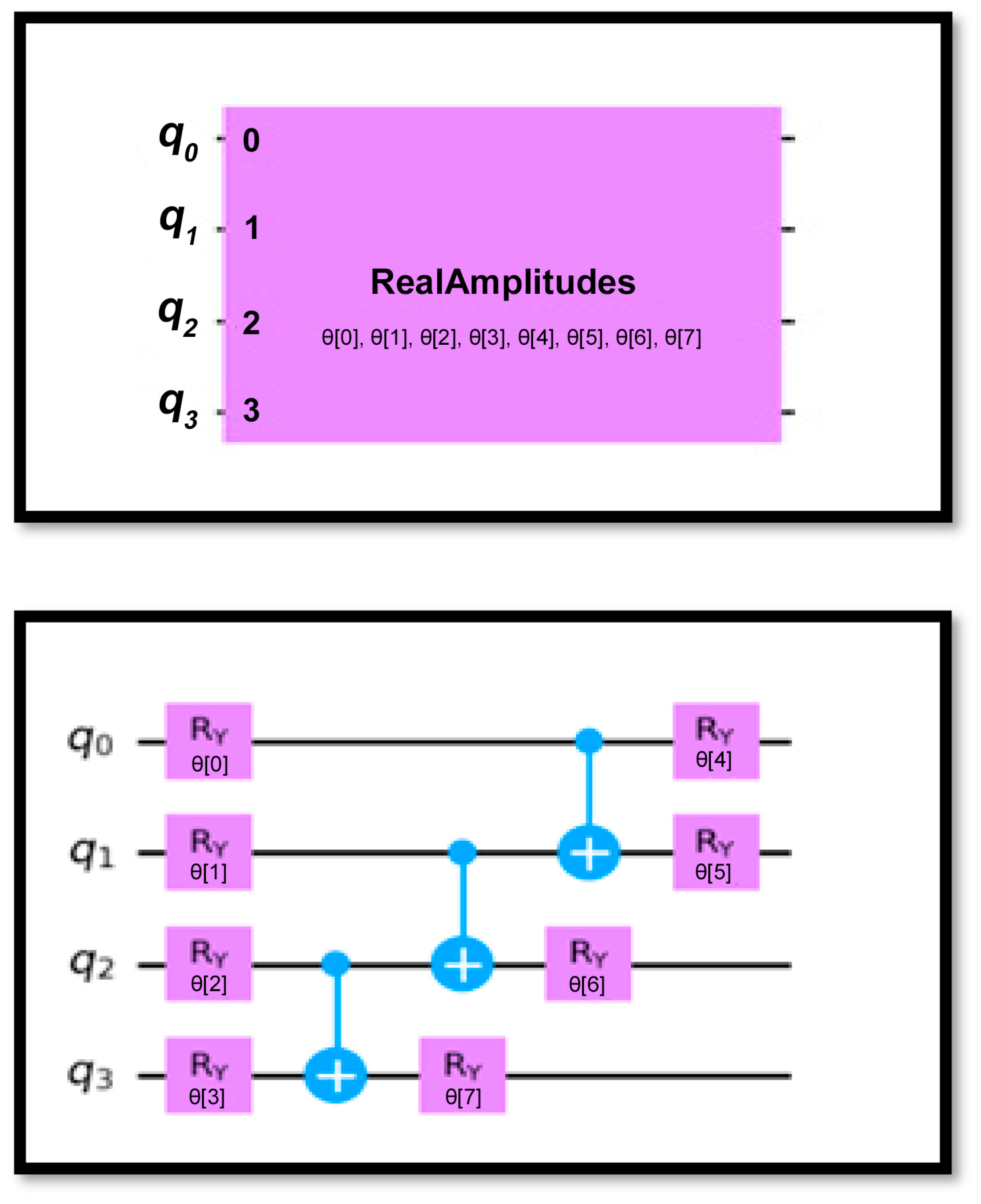
- Ansatz:
- The model employs a four-qubit Real Amplitudes ansatz with two layers of gates;
- In each layer, an RY gate is applied to each qubit with rotation angle θ;
- The rotation angles θ are adjusted iteratively during the optimization process to minimize the cost function;
- CNOT gates are applied to create entanglement between qubits [35].
- RY (θ) represents the rotation gate around the Y-axis with rotation angle θ;
- CNOT(j, j + 1) denotes the CNOT (Controlled-NOT) gate with control qubit j and target qubit j + 1;
- N is the number of qubits, four in this case.
- D.
- Cost function:
- E.
- Model Building:
- Data Visualization: matplotlib.pyplot and seaborn.
- Data Preprocessing: sklearn.preprocessing (StandardScaler, MinMaxScaler) for scaling, sklearn.model_selection (train_test_split) for splitting, and sklearn.decomposition (PCA) for dimensionality reduction.
- Performance Evaluation: sklearn.metrics.
- Quantum Computing: qiskit for circuit design and simulation and qiskit_machine_learning (NeuralNetworkClassifier, CircuitQNN) for quantum neural network implementation.
- Optimization: qiskit.algorithms.optimizers (L-BFGS-B, COBYLA, ADAM).
4. Optimizers
4.1. COBYLA
4.2. L_BFGS_B
4.3. ADAM
5. Comparative Analysis
5.1. Performance Evaluation
- Accuracy
- 2.
- Precision
- 3.
- Recall (Sensitivity)
- 4.
- F1 Score
5.2. COBYLA Optimizer
5.3. L_BFGS_B Optimizer
5.4. ADAM Optimizer
- Accuracy: COBYLA emerged as the top performer with an impressive accuracy rate of 92%, making it the most reliable optimizer for this task. L-BFGS-B followed with a respectable accuracy of 89%, while ADAM lagged significantly behind at 52%. This stark difference underscores COBYLA’s superiority in correctly classifying instances.
- Precision: Precision measures the proportion of true positive predictions among all positive classifications. COBYLA led once again with a precision rate of 89%, demonstrating its ability to effectively minimize false positives. L-BFGS-B achieved a slightly lower precision of 86%, maintaining reasonable performance. In contrast, ADAM exhibited a markedly low precision of 53%, indicating a high rate of incorrect positive predictions.
- Recall (Sensitivity): Recall evaluates a model’s ability to identify all actual positive instances. Both COBYLA and ADAM achieved a recall rate of 97%, showcasing their efficiency in minimizing false negatives. L-BFGS-B trailed slightly with a recall of 94%, which, while still strong, suggests a marginally higher tendency to miss positive cases.
- F1 Score: F1 score provides a balanced measure of precision and recall, offering insight into the overall effectiveness of a model. COBYLA achieved the highest F1 score of 93%, reflecting its superior ability to balance these two critical metrics. L-BFGS-B exhibited an F1 score of 90%, indicating a good performance but falling short of COBYLA’s optimization capabilities. ADAM achieved the lowest value of 68% on the F1 score.
- Convergence: The performance of the optimizers reveals distinct differences in loss, despite all three—L-BFGS-B, COBYLA, and ADAM—achieving 100% convergence.
- Loss: COBYLA demonstrated the lowest loss at 8.20%, indicating superior optimization in this context. L-BFGS-B resulted in a loss of 11.48%, which is notably higher than COBYLA’s. In contrast, ADAM exhibited a significantly elevated loss of 47.54%.
- Discussion
- COBYLA consistently outperformed the other optimizers across all metrics, achieving the highest accuracy (92%), precision (89%), and F1 score (93%). Its recall rate of 97%, tied with ADAM’s, indicates a good ability to minimize false negatives. Additionally, achieving the minimum loss in just 1 min of training, COBYLA is the most computationally efficient optimizer, solidifying its position as the optimal choice for this model.
- L-BFGS-B demonstrated moderate performance, with accuracy (89%) and recall (94%) values slightly lower than COBYLA’s. While it achieved a precision of 86%, its overall F1 score (90%) indicated balanced but less effective performance compared to COBYLA. Its training time of 6 min was longer than COBYLA’s, though still reasonable. Additionally, the loss for L-BFGS-B was 11.48%, indicating a less effective optimization compared to COBYLA’s loss but significantly better than ADAM’s loss.
- ADAM’s performance was notably weaker, particularly in terms of accuracy (52%) and precision (53%). Despite achieving a high recall rate of 97%, comparable to COBYLA’s, its poor precision resulted in an imbalanced model, as reflected in the F1 score of 68%. This pattern, characterized by high recall at the expense of precision, often indicates a strong bias towards predicting the positive class, where the model effectively captures most actual positives but incurs a significant number of false positives, ultimately leading to suboptimal overall accuracy. Furthermore, ADAM exhibited the longest training time of 10 min among the three optimizers, rendering it the least efficient choice in this context. Adding to its poor performance, ADAM demonstrated a significantly higher loss of 47.54%, indicating a substantial discrepancy between predicted and actual outcomes compared to both COBYLA’s 8.20% and L-BFGS-B’s 11.48% loss.
6. Conclusions and Future Work
Author Contributions
Funding
Institutional Review Board Statement
Informed Consent Statement
Data Availability Statement
Conflicts of Interest
References
- Marella, S.T.; Parisa, H.S.K. Introduction to Quantum Computing. In Quantum Computing and Communications; IntechOpen: London, UK, 2020; p. 61. [Google Scholar]
- Herman, D.; Googin, C.; Liu, X.; Galda, A.; Safro, I.; Sun, Y.; Pistoia, M. A survey of quantum computing for finance. arXiv 2022, arXiv:2201.02773. [Google Scholar]
- Ding, C.; Bao, T.-Y.; Huang, H.-L. Quantum-Inspired Support Vector Machine. IEEE Trans. Neural Netw. Learn. Syst. 2022, 33, 7210–7222. [Google Scholar] [CrossRef] [PubMed]
- Deutsch, D.; Jozsa, R. Rapid solution of problems by quantum computation. Proc. R. Soc. London. Ser. A Math. Phys. Sci. 1992, 439, 553–558. [Google Scholar]
- Shor, P.W. Algorithm for Quantum Computation: Discrete Logarithms and Factoring. In Proceedings of the 35th Annual Symposium on Foundations of Computer Science, Santa Fe, NM, USA, 20–22 November 1994; Volume 35, pp. 124–134. [Google Scholar]
- Abhijith, J.; Adedoyin, A.; Ambrosiano, J.; Anisimov, P.; Casper, W.; Chennupati, G.; Coffrin, C.; Djidjev, H.; Gunter, D.; Karra, S.; et al. Quantum Algorithm Implementations for Beginners. ACM Trans. Quantum Comput. 2022, 3, 1–92. [Google Scholar]
- Khan, T.M.; Robles-Kelly, A. Machine Learning: Quantum Vs Classical. IEEE Access 2020, 8, 219275–219294. [Google Scholar] [CrossRef]
- Huang, H.Y.; Broughton, M.; Mohseni, M.; Babbush, R.; Boixo, S.; Neven, H.; McClean, J.R. Power of data in quantum machine learning. Nat. Commun. 2021, 12, 2631. [Google Scholar] [CrossRef] [PubMed]
- Schuld, M.; Killoran, N. Quantum machine learning in feature Hilbert spaces. Phys. Rev. Lett. 2019, 122, 040504. [Google Scholar] [CrossRef]
- Chakraborty, S.; Das, T.; Sutradhar, S.; Das, M.; Deb, S. An Analytical Review of Quantum Neural Network Models and Relevant Research. In Proceedings of the 5th International Conference on Communication and Electronics Systems (ICCES), Coimbatore, India, 10–12 June 2020. [Google Scholar]
- Cerezo, M.; Arrasmith, A.; Babbush, R.; Benjamin, S.C.; Endo, S.; Fujii, K.; McClean, J.R.; Mitarai, K.; Yuan, X.; Cincio, L.; et al. Variational quantum algorithms. Nat. Rev. Phys. 2021, 3, 625–644. [Google Scholar] [CrossRef]
- Qin, J. Review of Ansatz Designing Techniques for Variational Quantum Algorithms. J. Phys. Conf. Ser. 2023, 2634, 012043. [Google Scholar] [CrossRef]
- Lubasch, M.; Joo, J.; Moinier, P.; Kiffner, M. Variational quantum algorithms for nonlinear problems. Phys. Rev. 2020, 101, 010301. [Google Scholar] [CrossRef]
- Kouda, N.; Matsui, N.; Nishimura, H.; Peper, F. Qubit neural network and its learning efficiency. Neural Comput. Appl. 2005, 14, 114–121. [Google Scholar] [CrossRef]
- Jeswal, S.K.; Chakraverty, S. Recent Developments and Applications in Quantum Neural Network: A Review. Arch. Comput. Methods Eng. 2019, 26, 793–807. [Google Scholar] [CrossRef]
- Chalumuria, A.; Kuneb, R.; Manoja, B.S. Training an Artificial Neural Network Using Qubits as Artificial Neurons: A Quantum Computing Approach. Procedia Comput. Sci. 2020, 171, 568–575. [Google Scholar] [CrossRef]
- Garcíaa, D.P.; Cruz-Benito, J. Systematic Literature Review: Quantum Machine Learning and its applications. Comput. Sci. Rev. 2022, 51, 100619. [Google Scholar] [CrossRef]
- Nielsen, M.A.; Chuang, I.L. Quantum Computation and Quantum Information, 1st ed.; Massachusetts Institute of Technology: Cambridge, MA, USA, 2004. [Google Scholar]
- Ezhov, A.A.; Ventura, D. Quantum neural Networks. In Future Directions for Intelligent Systems and Information Sciences; Springer: Berlin/Heidelberg, Germany, 2000; pp. 213–235. [Google Scholar]
- Khan, W.R.; Kamran, M.A.; Khan, M.U.; Ibrahim, M.M.; Kim, K.S.; Ali, M.U. Diabetes Prediction Using an Optimized Variational Quantum Classifier. Int. J. Intell. Syst. 2025, 2025, 1351522. [Google Scholar] [CrossRef]
- Yi, Z. Evaluation and Implementation of Convolutional Neural Networks. In Proceedings of the 1st International Conference on Advanced Algorithms and Control Engineering, Pingtung, Taiwan, 10–12 August 2018. [Google Scholar]
- Zhu, D.; Linke, N.M.; Benedetti, M.; Landsman, K.A.; Nguyen, N.H.; Alderete, C.H.; Perdomo-Ortiz, A.; Korda, N.; Garfoot, A. Training of quantum circuits on a hybrid quantum computer. Sci. Adv. 2019, 5, eaaw9918. [Google Scholar] [CrossRef]
- Ajibosin, S.S.; Cetinkaya, D. Implementation and Performance Evaluation of Quantum Machine Learning Algorithms for Binary Classification. Software 2024, 3, 498–513. [Google Scholar] [CrossRef]
- Al-Zafar Khan, M.; Al-Karaki, J.; Omar, M. Predicting Water Quality using Quantum Machine Learning: The Case of the Umgeni Catchment (U20A) Study Region. arXiv 2024, arXiv:2411.18141. [Google Scholar]
- Aminpour, S.; Banad, Y.; Sharif, S. Strategic Data Re-Uploads: A Pathway to Improved Quantum Classification Data Re-Uploading Strategies for Improved Quantum Classifier Performance. arXiv 2024, arXiv:2405.09377. [Google Scholar]
- Preskill, J. Quantum computing in the NISQ era and beyond. Quantum 2018, 2, 79. [Google Scholar] [CrossRef]
- Chaudhury, S.; Yamasaki, T. Robustness of Adaptive Neural Network Optimization Under Training Noise. IEEE Access 2021, 9, 37039–37053. [Google Scholar] [CrossRef]
- Abohashima, Z.; Elhoseny, M.; Houssein, E.H.; Mohamed, M. Classification with Quantum Machine Learning: A survey. arXiv 2020, arXiv:2006.12270. [Google Scholar]
- UC Irvine Machine Learning Repositroy. Heart Disease. 1988. Available online: https://archive.ics.uci.edu/dataset/45/heart+disease (accessed on 4 November 2023).
- Garate-Escamila, A.K.; ELHassani, A. Classification models for heart disease prediction using feature selection and PCA. Inform. Med. Unlocked 2020, 19, 100330. [Google Scholar] [CrossRef]
- Shrestha, D. Advanced Machine Learning Techniques for Predicting Heart Disease: A Comparative Analysis Using the Cleveland Heart Disease Dataset. Appl. Med. Inform. 2024, 46, 91–102. [Google Scholar]
- Han, J.; Kamber, M.; Pei, J. Data Mining: Concepts and Technique, The Morgan Kaufmann Series in Data Management Systems, 3rd ed.; Elsevier: Amsterdam, The Netherlands, 2012. [Google Scholar]
- Medium. Building a Quantum Variational Classifier Using Real-World Data. Qiskit. 2021. Available online: https://medium.com/qiskit/building-a-quantum-variational-classifier-using-real-world-data-809c59eb17c2 (accessed on 2 February 2024).
- IBM Quantum Documentation. RealAmplitudes. Available online: https://docs.quantum.ibm.com/api/qiskit/0.30/qiskit.circuit.library.RealAmplitudes (accessed on 1 February 2024).
- Mangini, S. Variational Quantum Algorithms for Machine Learning Theory and Applications. Ph.D. Thesis, University of Pavia, Pavia, Italy, 2023. [Google Scholar]
- Terven, J.; Cordova-Esparza, D.M.; Ramirez-Pedraza, A.; Chavez-Urbiola, E.A.; Romero-Gonzalez, J.A. Loss Functions and Metrics in Deep Learning. arXiv 2023, arXiv:2307.02694. [Google Scholar]
- Desai, C. Comparative Analysis of Optimizers in Deep Neural Networks. Int. J. Innov. Sci. Res. Technol. 2020, 5, 959–962. [Google Scholar]
- Vishwakarma, N. What is Adam Optimizer? 2024. Available online: https://www.analyticsvidhya.com/blog/2023/09/what-is-adam-optimizer/#:~:text=The%20Adam%20optimizer%2C%20short%20for,Stochastic%20Gradient%20Descent%20with%20momentum (accessed on 8 January 2024).
- Zhu, C.; Byrd, R.H.; Lu, P.; Nocedal, J. Algorithm 778: L-BFGS-B: Fortran subroutines for large-scale bound-constrained optimization. ACM Trans. Math. Softw. (TOMS) 1997, 23, 550–560. [Google Scholar] [CrossRef]
- Zamyshlyaeva, A.A.; Bychkov, E.V.; Kashcheeva, A.D. Algorithm for Numerical Solution of the Optimal Control Problem for One Hydrodynamics Model Using the COBYLA Method. J. Comput. Eng. Math. 2024, 11, 40–47. [Google Scholar]
- Powers, T.; Rajapakse, R.M. Using Variational Eigensolvers on Low-End Hardware to Find the Ground State Energy of Simple Molecules. Quantum Physics. arXiv 2023, arXiv:2310.19104. [Google Scholar]
- Wendorff, A.; Botero, E.; Alonso, J.J. Comparing Different Off-the-Shelf Optimizers’ Performance in Conceptual Aircraft Design. In Proceedings of the 17th AIAA/ISSMO Multidisciplinary Analysis and Optimization Conference, Washington, DC, USA, 13–17 June 2016. [Google Scholar]
- IBM Quantum Documentation. L_BFGS_B. Available online: https://docs.quantum.ibm.com/api/qiskit/0.40/qiskit.algorithms.optimizers.L_BFGS_B (accessed on 1 December 2024).
- Su, Y.; Song, K.; Yu, K.; Hu, Z.; Jin, H. Quantitative Study of Predicting the Effect of the Initial Gap on Mechanical Behavior in Resistance Spot Welding Based on L-BFGS-B. Materials 2024, 17, 4746. [Google Scholar] [CrossRef]
- Brownlee, J. Gentle Introduction to the Adam Optimization Algorithm for Deep Learning. Deep Learning Performance. 2021. Available online: https://machinelearningmastery.com/adam-optimization-algorithm-for-deep-learning/ (accessed on 26 November 2024).
- Ruder, S. An overview of gradient descent optimization. arXiv 2017, arXiv:1609.04747. [Google Scholar]
- Pellow-Jarman, A.; Sinayskiy, I.; Pillay, A.; Petruccione, F. A comparison of various classical optimizers for a variational quantum linear solver. Quantum Inf. Process. 2021, 20, 202. [Google Scholar] [CrossRef]


| Optimizer | Accuracy | Precision | Recall | F1 Score | Training Time | Converges | Loss |
|---|---|---|---|---|---|---|---|
| COBYLA | 92% | 89% | 97% | 93% | 1 | 100% | 8.20% |
| L-BFGS-B | 89% | 86% | 94% | 90% | 6 | 100% | 11.84% |
| ADAM | 52% | 53% | 97% | 68% | 10 | 100% | 47.54% |
| Optimizer | True Positive | False Positive | False Negative | True Negative |
|---|---|---|---|---|
| COBYLA | 25 | 4 | 1 | 31 |
| L-BFGS-B | 24 | 5 | 2 | 30 |
| ADAM | 1 | 28 | 1 | 31 |
Disclaimer/Publisher’s Note: The statements, opinions and data contained in all publications are solely those of the individual author(s) and contributor(s) and not of MDPI and/or the editor(s). MDPI and/or the editor(s) disclaim responsibility for any injury to people or property resulting from any ideas, methods, instructions or products referred to in the content. |
© 2025 by the authors. Licensee MDPI, Basel, Switzerland. This article is an open access article distributed under the terms and conditions of the Creative Commons Attribution (CC BY) license (https://creativecommons.org/licenses/by/4.0/).
Share and Cite
AL Ajmi, N.A.; Shoaib, M. Optimization Strategies in Quantum Machine Learning: A Performance Analysis. Appl. Sci. 2025, 15, 4493. https://doi.org/10.3390/app15084493
AL Ajmi NA, Shoaib M. Optimization Strategies in Quantum Machine Learning: A Performance Analysis. Applied Sciences. 2025; 15(8):4493. https://doi.org/10.3390/app15084493
Chicago/Turabian StyleAL Ajmi, Nouf Ali, and Muhammad Shoaib. 2025. "Optimization Strategies in Quantum Machine Learning: A Performance Analysis" Applied Sciences 15, no. 8: 4493. https://doi.org/10.3390/app15084493
APA StyleAL Ajmi, N. A., & Shoaib, M. (2025). Optimization Strategies in Quantum Machine Learning: A Performance Analysis. Applied Sciences, 15(8), 4493. https://doi.org/10.3390/app15084493