Featured Application
This work is directly applied to optimize the performance of heliostat fields used in solar concentrating facilities.
Abstract
In this work, solar concentrating heliostat fields are modeled using accurate solar-tracking algorithms and a wide range of rotation models to investigate the parameters controlling the mechanical efficiency of these solar facilities. Iterative procedures are first described to determine the rotation angles needed to properly orient a single heliostat for the most commonly used mechanical models, including the azimuth-elevation, tilt-roll, and target-aligned models. These mathematical techniques were integrated into our Light Analysis Modelling (LAM) software and used to study a realistic heliostat field with six different mechanical rotation models for the full year of 2024 and a daily working range of 08:00–16:00 Local Time (LCT). Two locations were chosen, representing the highest and lowest latitudes from the SFERA-III EU list of solar concentrating facilities with heliostat fields: Jülich (Germany) and Protaras (Cyprus). The results obtained show that tilt-roll models require less angular rotation (−15.2% in Jülich, −20.2% in Protaras) and a narrower angular range (−14.5% in Jülich, −20.2% in Protaras) than azimuth-elevation models. Seldom-used target-aligned models are more efficient with tilt-roll rotations (compared with the tilt-roll model: −35.1% rotations in Jülich, −29.2% in Protaras; −12.3% angular range in Jülich, −14.3% in Protaras) and less efficient with azimuth-elevation rotations (compared with the azimuth-elevation model: +53.2% rotations in Jülich, +39.2% in Protaras; +96.2% angular range in Jülich, +87.5% in Protaras).
1. Introduction
Concentrating solar power (CSP) technologies are promising renewable energy systems with high exergy efficiency [1,2] and a comparatively low environmental footprint. Modern solar thermal power plants consist of a solar tower or a central receiver system equipped with a field of heliostats that reflect (re-direct) the so-called DNI (direct normal irradiance) onto a central receiver mounted at the top of a tower [3]. Each heliostat is a two-axis tracking system with an almost flat mirrored surface. However, historically, the first heliostats were used in another type of point-focusing concentrating solar technology: the solar furnace. In fact, in an article published in 1958, Hughes [4] described a two-component solar furnace, a condenser–heliostat combination, in which the condenser faces downward at 30° towards a heliostat comprised of numerous rows of plane mirrors mounted on a horizontal turntable. The world’s first solar tower plant was equipped with a field of point-focus Fresnel mirrors, and it was built and tested at Sant’Ilario, near Genoa (Italy), in 1965 [5]. Using almost flat mirrors and following four decades of prototype test facilities built around the world, solar tower or central receiver plants only started gaining large commercial momentum with Abengoa‘s PS10 in 2007 [6], followed by other plants, like Gemasolar (also located in the Spanish province of Andalucia), which was commissioned in 2011 [7].
Computer modeling of CSP facilities, namely those with a heliostat field, can be an invaluable tool for improving their efficiency, allowing us to better understand and simplify their inner mechanisms. In the literature, there are several examples of studies that present interesting findings, not only concerning blocking and shading effects, e.g., [8,9,10], but also analyzing the mechanical rotations of the heliostats, e.g., [11,12,13,14]. More recently, generative deep learning models have been used to predict heliostat surfaces from target images [15], and novel pointing correction techniques based on nonlinear Limit Cycle Oscillators (LCOs) have been applied to the digital twin [16] of a heliostat field.
In this manuscript, computer simulations of heliostat fields are reported, specifically those looking into the mechanical rotations needed to properly orient the heliostat mirrors. These studies allow for the assessment of the overall efficiency of the various models (equivalent studies covering optical aspects were reported in a previous publication [17]).
Simple mathematical models are introduced to simulate the most common mirror orientation models, which involve two rotation axes: azimuth-elevation, tilt-roll, and target-aligned. Simple layouts to represent realistic heliostat fields are then suggested and simulated.
The number of ray-tracing computer packages currently available to model optical systems is vast, ranging from software commonly used to model CSP systems (Tonathium [18], SolTrace [19]) to general-purpose optical software designed to project complex optical devices, including lenses (FRED [20], Zemax [21], Code V [22], LightTools [23], TracePro [24]). Tonathium and SolTrace are distributed as open-source software (available from the GitHub repository). All other packages are commercially available from the cited companies.
However, the software used in this work was specifically written for these studies, providing maximum control, flexibility, efficiency, and accuracy, thus increasing our knowledge and error detection capacity. This software includes the algorithms recently reported [25] to calculate the sun’s position (as a function of time, date, latitude, and longitude), which are essential for the work reported here. Code to detect shading and blocking effects, as well as mechanical collisions and to implement attenuation effects, has also been applied throughout this work. It would be awkward to pursue these studies using standard software packages, given the challenges of interconnecting our input (simulation) and output (characterization) algorithms and requirements with those large computer packages.
2. Heliostat Orientation
Once the sun’s local position is known, the second step in modeling a working heliostat field is to properly orient each individual heliostat. This orientation depends on the heliostat’s location relative to the target, as well as the mechanical characteristics of the rotating device supporting the heliostat mirror. There are essentially three main designs used to rotate heliostats, as shown in Figure 1, all of which include a primary rotating axis (stronger, closer to the soil, colored purple) and a secondary rotating axis (lighter, closer to the mirror, colored green).
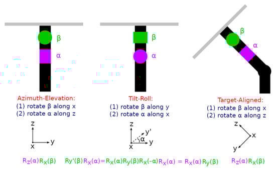
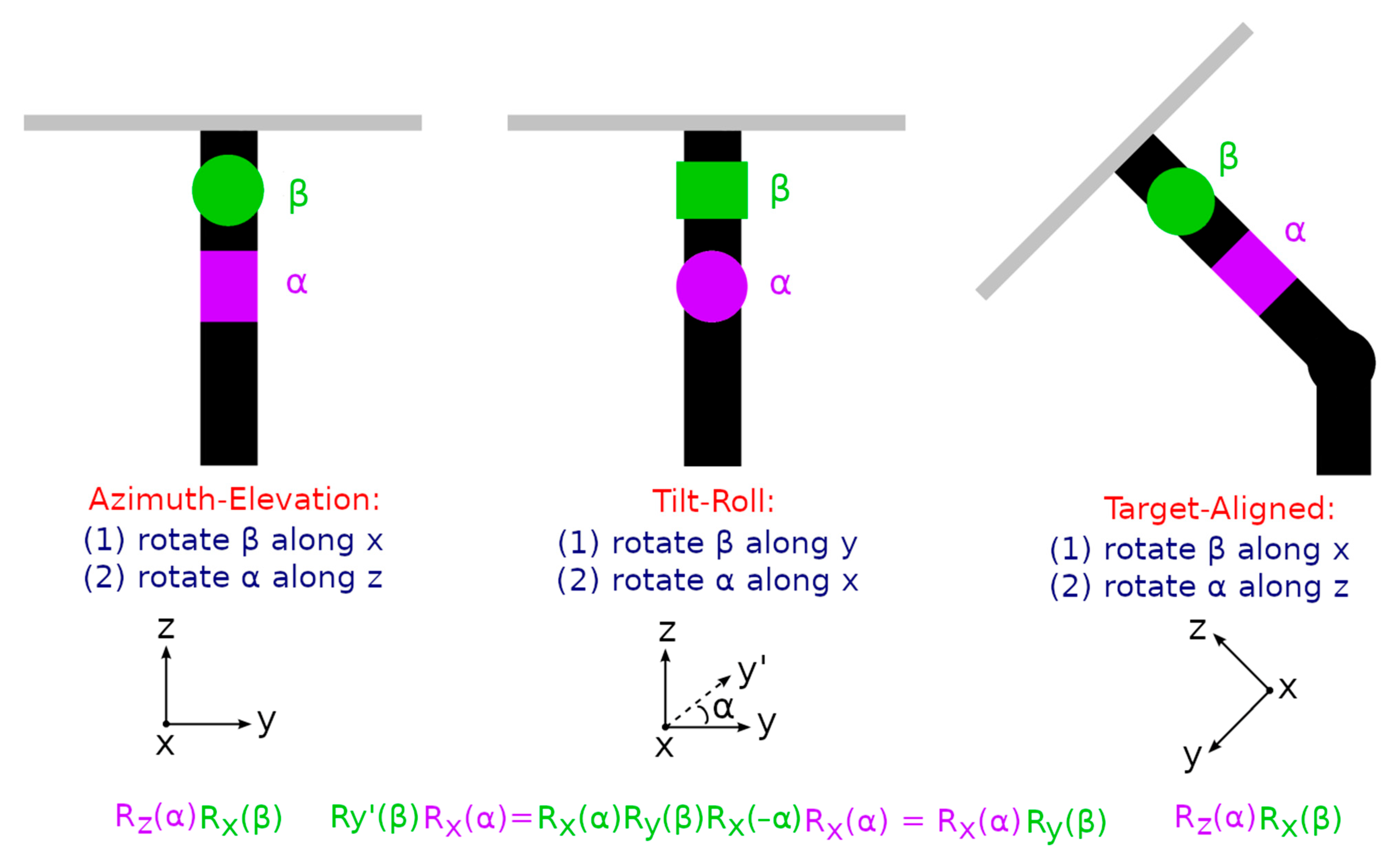
Figure 1.
Rotating axes, primary (α angle, purple color) and secondary (β angle, green color), for azimuth-elevation, tilt-roll, and target-aligned mechanical designs. The 3 layouts can be described by the product of two rotating matrices, around the orthogonal x, y, z axes.
- (1)
- The azimuth-elevation layout features a primary axis that points to the sky (along z) and a secondary axis that is horizontal (along x, initially pointing East). The secondary axis rotates by β first (to fix altitude), and then the primary axis rotates by α (to fix azimuth).
- (2)
- The tilt-roll layout features a primary axis that is horizontal (along x, typically pointing east) and a secondary axis (initially horizontal, along y, pointing north) that is attached to the mirror frame. The primary axis rotates by α first (to fix altitude, the tilt) and then the secondary axis, which rotates by β (around the tilted y’ axis, the roll). As shown in Figure 1, this mechanical two-rotation sequence is mathematically equivalent (including offsets) to first rotating the secondary axis (around y) and then the primary axis (around x). The so-called polar-oriented model [26] is obtained when the tilt-roll secondary axis points north and the primary axis points east.
- (3)
- The target-aligned layout is where the main axis and the heliostat mirror point directly to the target in the starting, resting position. This layout can be mathematically handled by converting the Earth referential to a target referential and then determining the orientation by applying either an azimuth-elevation or a tilt-roll approach to the mechanical rotations, as described above, before converting back to the Earth referential in the end.
2.1. Azimuth-Elevation (AE) Orientation
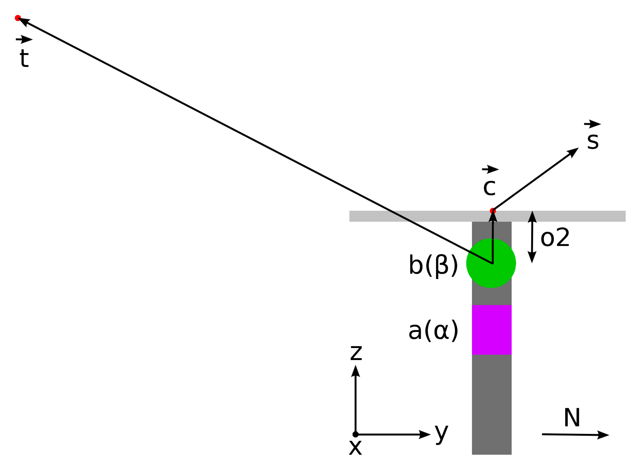
To obtain the mirror center and orientation, the following procedure can be applied, assuming that the heliostat initially points upwards and that the origin is at the intersection of axis a with axis b (see Figure 2):

Figure 2.
Model to orient an azimuth-elevation heliostat, showing fixed quantities (vector target , vector sun , offset o2) and variable quantities (vector , angles α, β, around axes a, b). Axes x, y, and z point east, north and toward the sky, respectively.
- (1)
- Using the vectors target, , center, , and sun, , calculate the unit normal vector, , as follows:
- (2)
- Using the normal vector, , calculate the rotating angles, α and β (around the z and x axes), as follows:
- (3)
- Using the rotating angles, α and β, and offset, o2, recalculate the center vector, , as follows:
- (4)
- Repeat steps 1, 2, and 3 until convergence is reached for the α and β angles and the normal and center vectors.
2.2. Tilt-Roll (TR) Orientation
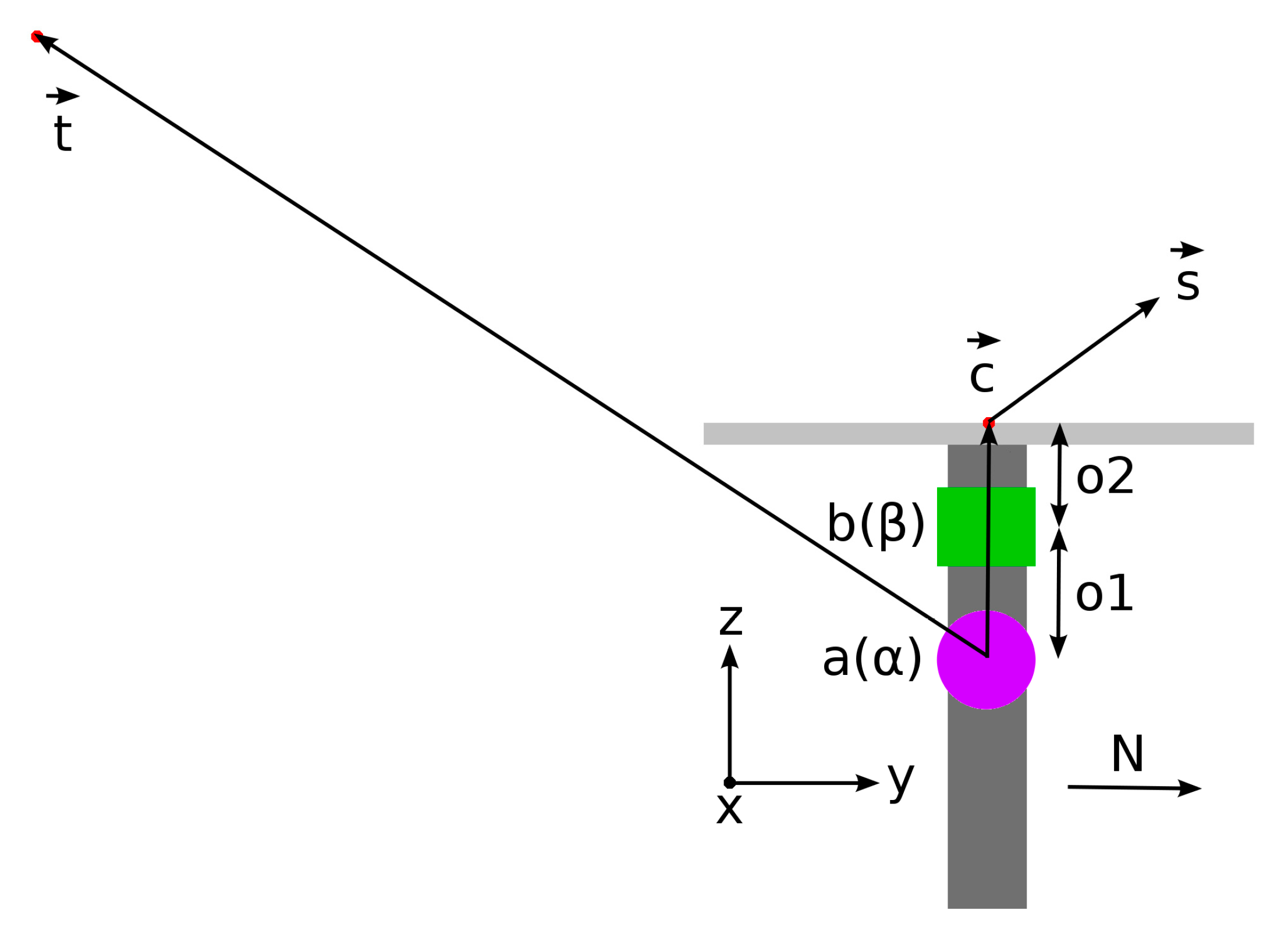
To obtain the mirror center and orientation, the following procedure can be applied, assuming that the heliostat initially points upward and the origin is at the intersection of the vertical axis with axis a (see Figure 3):
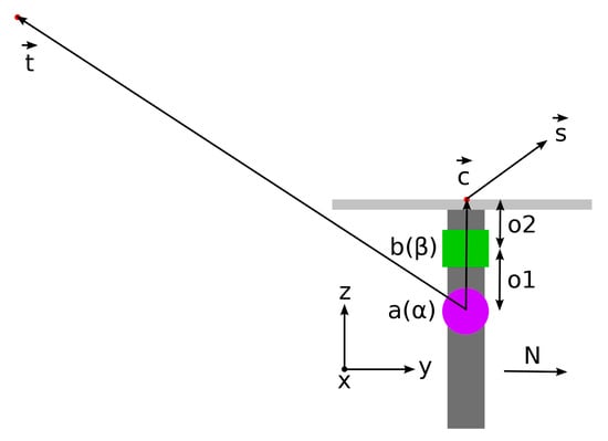
Figure 3.
Model to orient a tilt-roll heliostat, showing fixed quantities (vector target , vector sun , offsets o1, o2) and variable quantities (vector , angles α, β around axes a, b). Axes x, y, and z point east, north, and toward the sky, respectively.
- (1)
- Using the vectors target, , center, , and sun, , calculate the unit normal vector, , using Equation (1) introduced above.
- (2)
- Using the normal vector, , calculate the rotating angles, α and β (around the x and y axes), as follows:
- (3)
- Using the rotating angles, α and β and offsets, o1 and o2, recalculate the center vector, , as follows:
- (4)
- Repeat steps 1, 2, and 3 until convergence is reached for the α and β angles and the normal and center vectors.
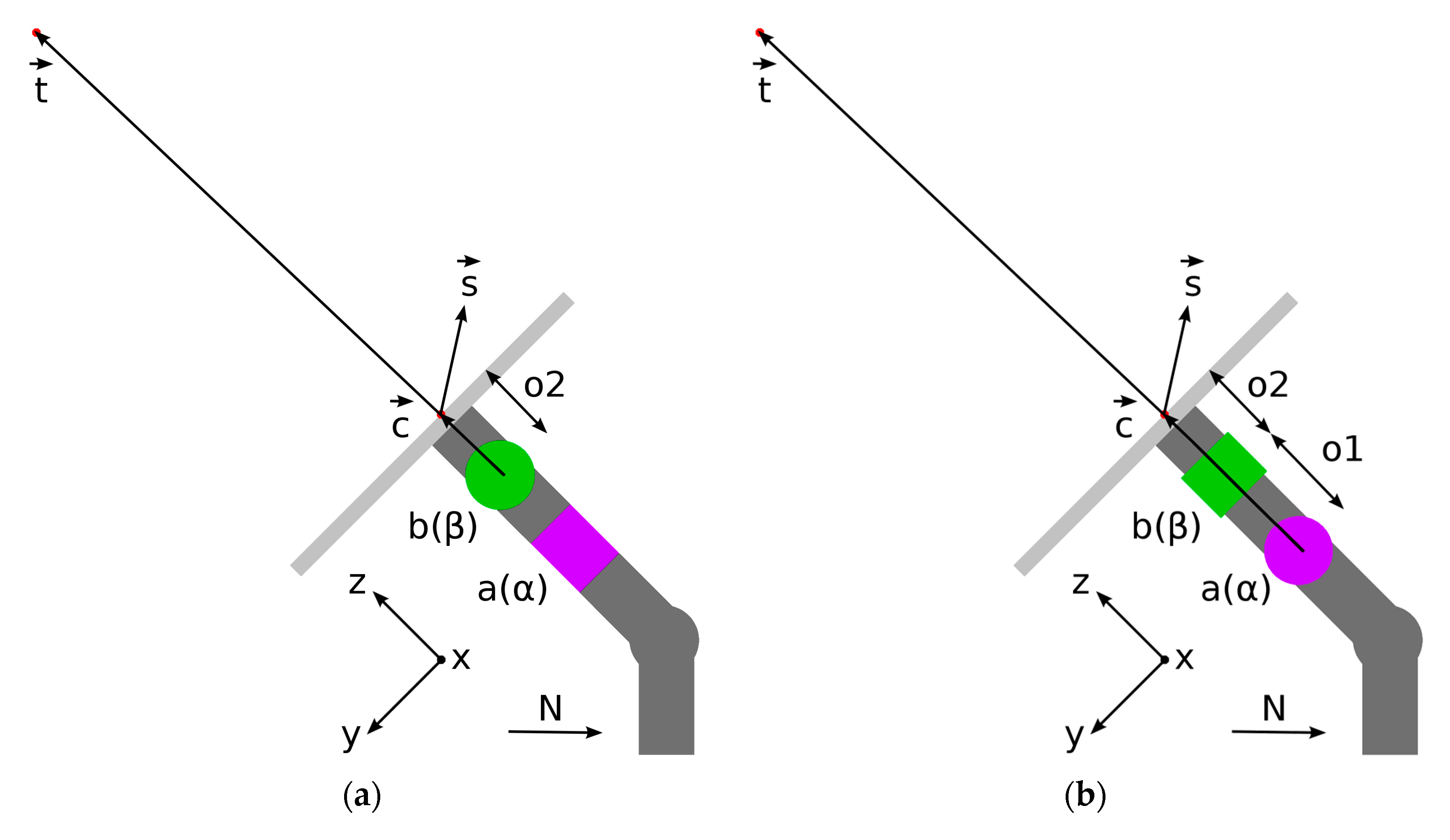
2.3. Target-Aligned (TA) Orientation
To obtain the mirror center and orientation, the following procedure can be applied, assuming that the heliostat initially points to the target and the local mechanical model is either azimuth-elevation or tilt-roll (see Figure 4). In the first case, the origin is at the secondary axis, b (in green), while in the second case, the origin is at the primary axis, a (in purple).

Figure 4.
(a) Azimuth-elevation and (b) tilt-roll mechanical models to orient a target-aligned heliostat, showing fixed quantities (vector target , vector sun , offsets o1, o2) and variable quantities (vector , angles α, β around axes a, b). Axis z points to the target and axis x points westerly.
- (1)
- Build the target referential as follows:
- (2)
- Convert the sun vector to the target referential as follows (target and center vectors are along the z axis):
- (3)
- Apply steps 1, 2, and 3 of the azimuth-elevation model or steps 1, 2, and 3 of the tilt-roll model until convergence is reached for the α and β angles. This can be accomplished because the new target-aligned xyz referential works exactly like the Earth sky-aligned xyz referential: first, rotate the secondary x-axis to fix the altitude, and then rotate the primary z-axis to fix the azimuth (the new elevation-azimuth model, referred to here as TA/AE); or first, rotate the secondary y-axis to fix azimuth, and then rotate the primary x-axis to fix altitude (the new tilt-roll model, referred to here as TA/TR).
- (4)
- Convert the normal and center vectors back to the Earth referential as follows:
There is a key difference between AE, TR heliostats (initially pointing to the sky) and TA/TE, TA/TR heliostats (initially pointing to the target) that should be noted. In the AE and TR models, the angle controlling altitude (β in AE, α in TR) is always positive. In the TA/AE and TA/TR models, this altitude angle can be positive or negative, depending on whether the sun is above or below the target, as seen from the heliostat. A negative β angle in the TA/AE model is handled by adding a 180° rotation to the α angle, as the mechanical system always assumes a positive β rotation. In the TA/TR model, there is no such solution, so the mechanical system must be able to handle a negative α rotation. In the TA/AE model, the allowed angular range is [−180°, 180°] for α and [0, 90°] for β. In the TA/TR model, the allowed angular range is [−90°, 90°] for α and [−90°, 90°] for β.
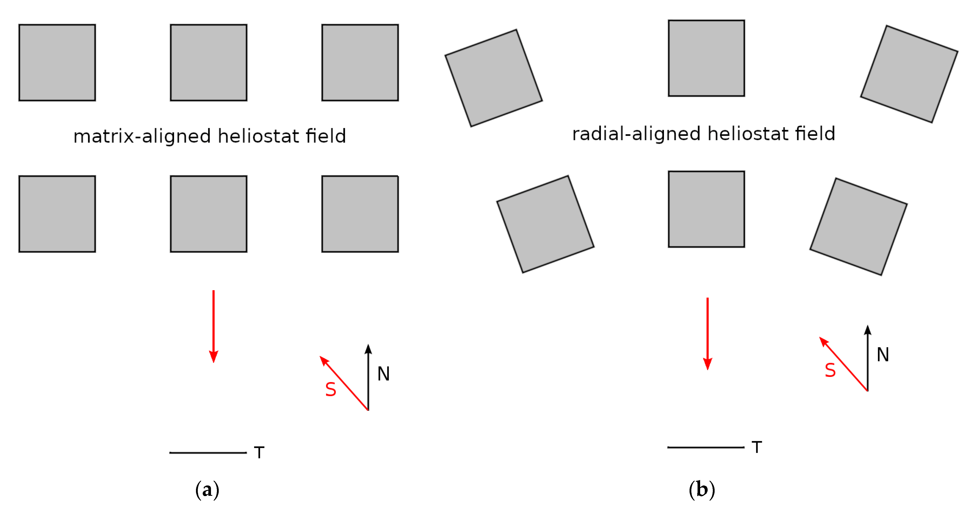
2.4. Radial Layout
The methods shown above for azimuth-elevation and tilt-roll models assume that for each heliostat, the y-axis points north and the x-axis points east, so heliostats are initially oriented in a matrix-aligned format (see Figure 5).
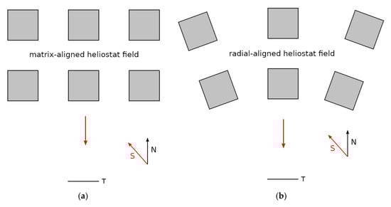
Figure 5.
Heliostat fields: (a) matrix-aligned; (b) radial-aligned. The target (T) points north (N), to collect the sun’s (S) rays reflected by the heliostats.
If heliostats are horizontally aligned with the target and oriented in a radial-aligned format, the new azimuth-elevation model (here named AE/TA) and the new tilt-roll model (here named TR/TA) can be handled by combining the iterative techniques described above for the target-aligned model (the new azimuth-elevation model can be handled by simply changing the primary axis rotation to accommodate the radial angle). If vector points to the heliostat center and vector points to the target, the following steps are taken:
- (1)
- Build the target referential as follows (vector y points from the target to the heliostat):
- (2)
- Convert the sun vector (plus target, center vectors) to the target referential, using Equation (7) introduced above.
- (3)
- Repeat steps 1, 2, and 3 of the azimuth-elevation model (AE/TA) or steps 1, 2, and 3 of the tilt-roll model (TR/TA) until convergence is reached for the α and β angles. In the second case, in the newly aligned referential, the model works exactly like the tilt-roll model in the Earth referential: first, rotate the secondary axis (rotating along the projected heliostat center-target axis), and then rotate the primary axis (rotating perpendicular to the projected heliostat center-target axis).
- (4)
- Convert the normal and center vectors back to the Earth referential, using Equations (8) and (9) introduced above.
For all six mechanical models discussed here (AE, TR, TA/AE, TA/TR, AE/TA, and TR/TA), for typical offsets of o1 (30 cm) and o2 (20 cm), fewer than 10 iterations are usually enough to achieve convergence, even for angle tolerances as strict as 10−10 rad (the number of iterations increases with offset). Finally, it should be emphasized that the radiation flux distribution collected at the target, resulting from the heliostat mirror reflection, is equal for these six mechanical models when properly applied (changes due to different mirror offsets, o1 and o2, are usually negligible).
3. Heliostat Reflection
To handle beam reflection, the heliostat should be rotated to a horizontal orientation, where all aspects related to ray generation, interception, and reflection are easily handled, and then rotated back to the original orientation. The procedure is as follows:
- (1)
- Find the rotation sequence, , that transforms a horizontal heliostat, which is given by , to the real heliostat orientation, which is given by . Use the inverse transformation, , to transform the sun vector to the horizontal referential as follows:
- (2)
- Generate the random ray position in the flat surface immediately above the horizontal heliostat and transform the incident sun vector to the reflected sun vector ). The actual reflection depends on the type of heliostat curvature (planar, spherical, parabolic), as discussed in [17]. The calculation involves the ray’s interception with the curved surface and the analytical calculation of the normal vector at that point to obtain the reflected vector [27,28]. The position (and slightly random orientation) of the incident Sun vector is calculated according to the astronomy algorithm reported previously [25].
- (3)
- Use the direct transformation, , to obtain, in the real heliostat orientation, the reflected sun vector and the ray position as follows:
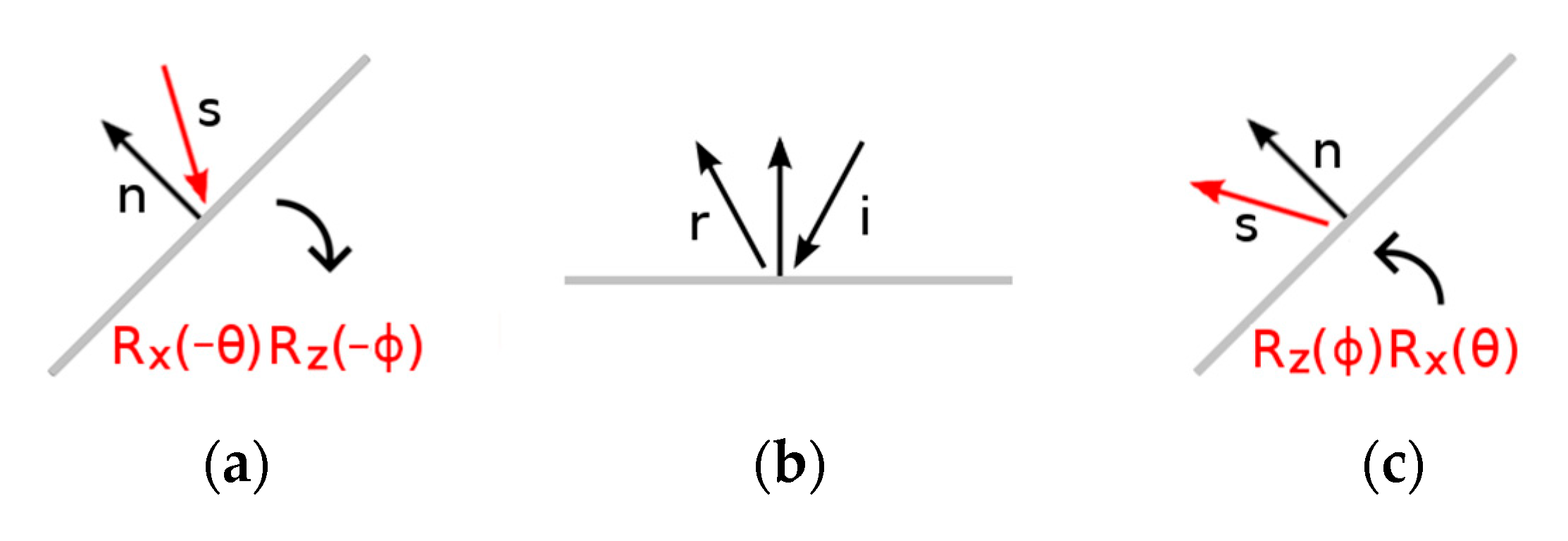
The overall mathematical sequence is shown in Figure 6. We note that these transformations are purely mathematical abstractions that can be applied to any mechanical model (we only need to know the normal vector for the oriented heliostat), unlike the operations reported above for azimuth-elevation, tilt-roll, and target-aligned models, which describe actual mechanical rotations.
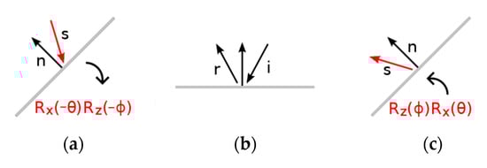
Figure 6.
Mathematical sequence to handle sun ray reflections at the heliostat curvature: (a) Use the inverse rotation sequence, , to obtain the incident sun vector in the horizontal heliostat; (b) Transform the incident sun ray (i) to the reflected ray (r); (c) Use the direct rotation sequence, , to obtain the reflected sun vector in the real heliostat.
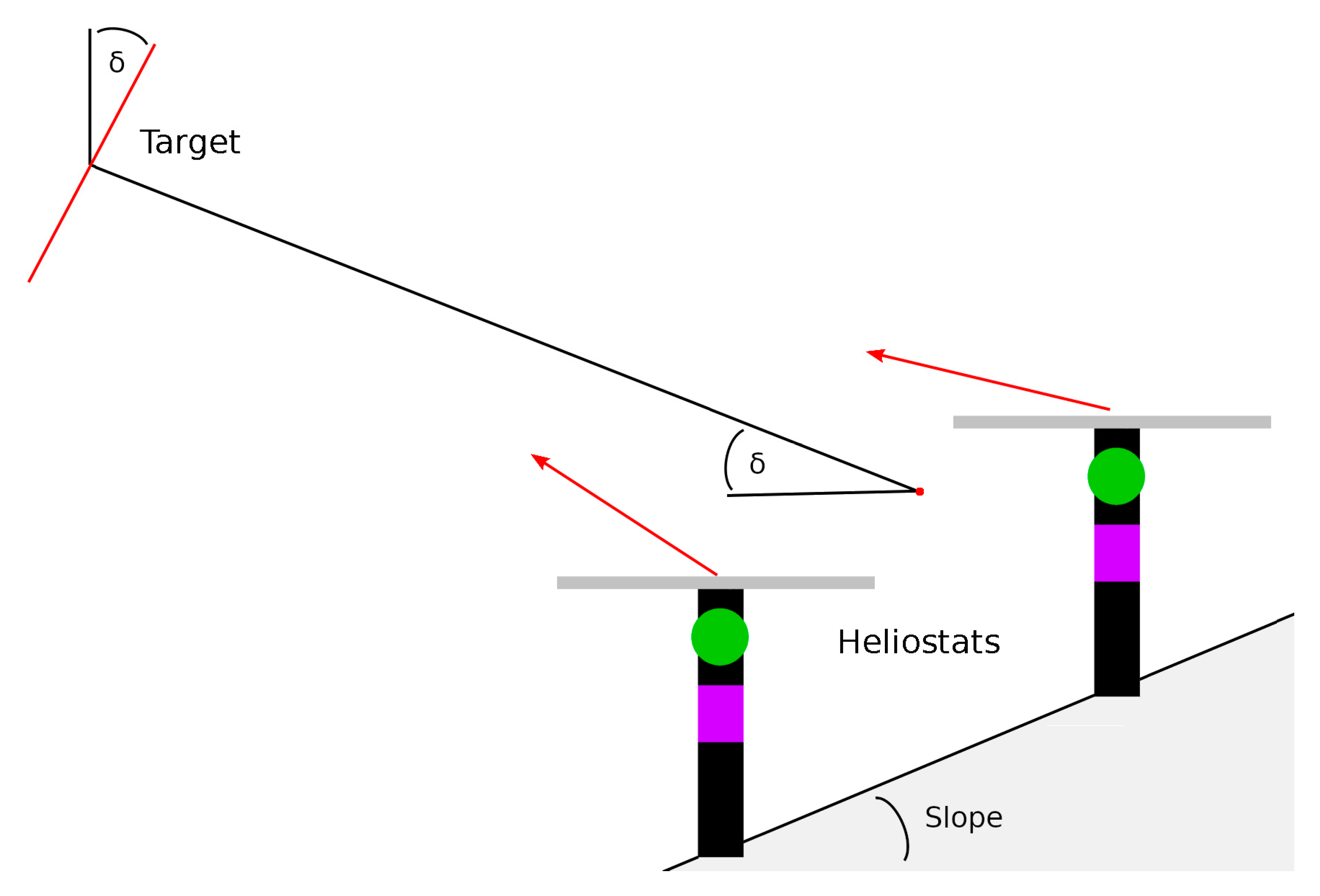
4. Target Detector
To collect light rays intercepting the target, we use a pixel-based rectangle, which is characterized by its position, normal, and up vectors (like a photographic camera). Ideally, the target plane is oriented to be normal to the average direction of the rays coming from the heliostat field (see Figure 7). The data acquired is used to produce images, statistical data, and profiles, as extensively illustrated in our previous works [27,28,29].

Figure 7.
Pixel-based target rectangle (the collecting detector), perpendicular to the average sun radiation coming from the heliostat field (heliostats are represented in the rest position). The angle, δ, that the target should rotate depends of the heliostats layout and geometry, the ground slope, and the tower distance and height.
5. Computational Details
Unless we are studying an already existing heliostat field, many choices and compromises must be taken into account before designing the new model, as follows:
- (1)
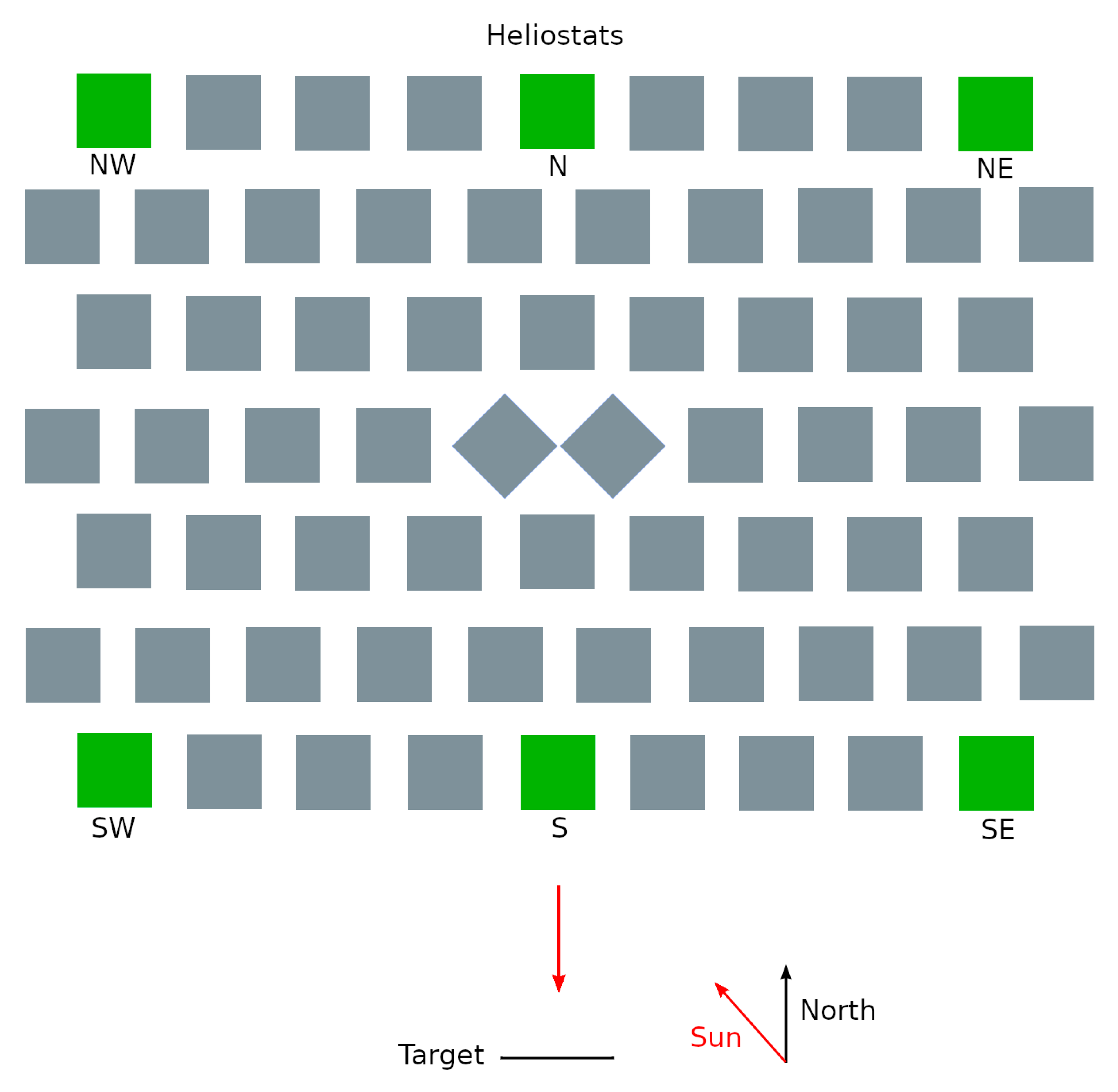
- How many heliostats should we model? Simulating the heliostat reflection and target collection through ray tracing requires significant computer time, so the number of heliostats investigated should be kept to a minimum. In this work, however, the research is concentrated on the mechanical rotations of the heliostats, so we only need to orient the heliostats. Therefore, the computer time required is much less than when studying shading/blocking effects. We choose to simulate the layout already used in our previous work [17] to obtain data results that are representative yet simple to analyze and report. This layout is shown in Figure 8, with a total of 66 heliostats in a staggering arrangement. Only the six end heliostats (in green, henceforth named SW, S, SE, NW, N, and NE) are independently oriented, as we identify them as representatives of the whole set.
 Figure 8. Layout for the simulated heliostat field, with 66 heliostats in a staggering arrangement. The target points north to collect the sun’s rays reflected. Only the 6 green heliostats are simulated. The heliostat mirrors are either square (2.0 m × 2.0 m, separated by 1.0 m in both north–south and east–west directions), as shown in this picture, or rectangular (2.5 m east–west × 1.6 m north–south, with 1.0 m separation east–west and 1.9 m north–south). The two central heliostats are rotated 45° to emphasize that they cannot touch.
 - (2)
- Shall we simulate a horizontal field or a field with a south–north slope angle of 10° or 20°? Using a slope is more interesting, but choosing a horizontal flat terrain is simpler, closer on average to real land conditions, and better emphasizes the differences between the front and back heliostat rows. In our previous work, we aimed to study shading/blocking effects, so we extensively investigated 0° and 10° slopes [17]. In this work on mechanical rotations, we want to avoid shading/blocking as much as possible, so we always used the more favorable 10° slope.
- (3)
- Should we use square or rectangular heliostats? Additionally, what dimensions should we use? Larger sizes provide more radiant energy but are less flexible to handle and require stronger mechanical structures to withstand the wind. Rectangular heliostats might handle wind better than square heliostats of the same area due to their lower height. In our previous work, we investigated square 2.0 m × 2.0 m and rectangular 2.5 m × 1.6 m heliostats, both with an area of 4 m2 each (typical sizes in tilt-roll heliostat fields). In this work, we used both geometries (see Figure 9); however, for the mechanical rotation studies, the rectangular heliostats were chosen because they seem to be less affected by shading/blocking effects [17].
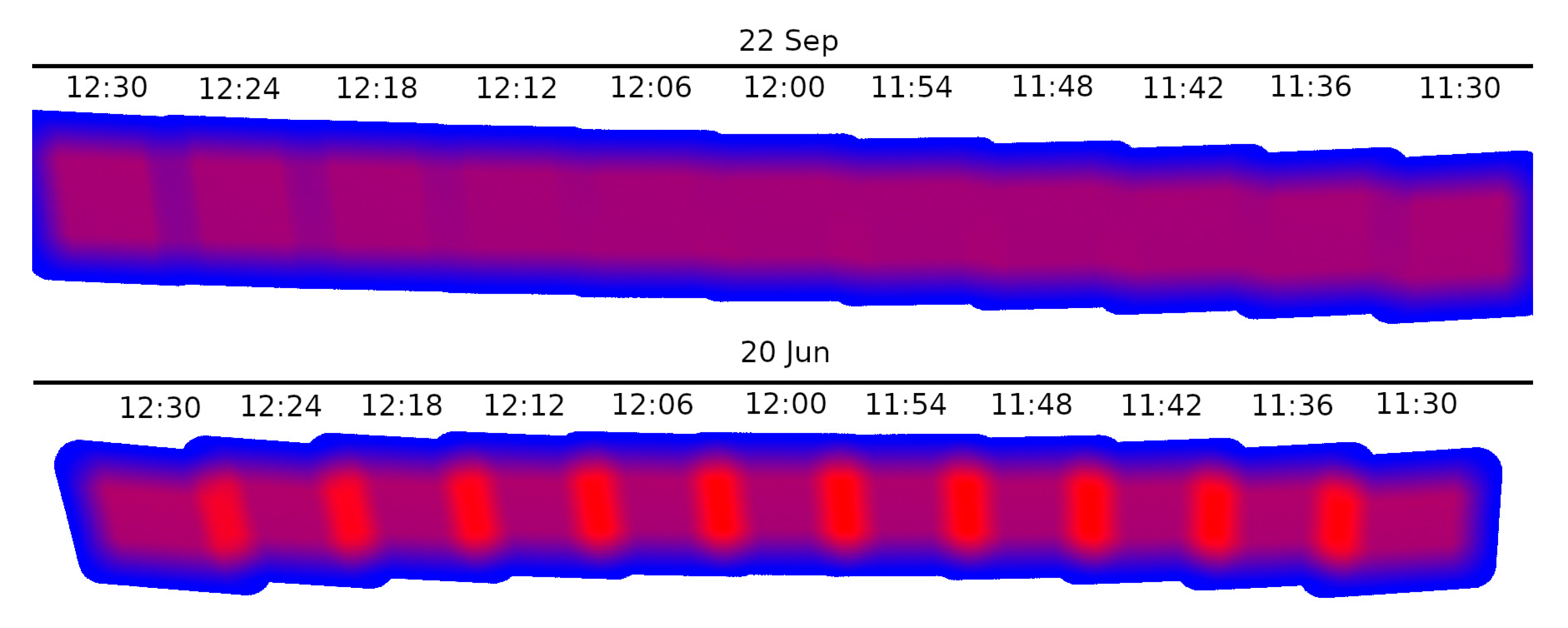
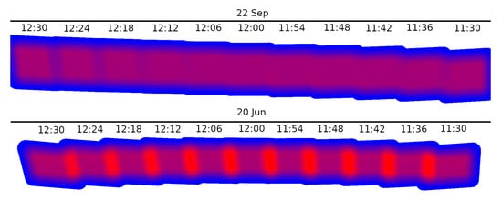 Figure 9. Radiation collected at the target screen (represented in a blue–red scale accounting for minimum–maximum intensity) after the reflection of the N heliostat (see Figure 7 and Figure 8), calculated with 108 ray tracing events. The square (2.0 m × 2.0 m) heliostat is fixed and aligned with the target center at 12:00 LCT. The radiation successively received in the target from 11:30 to 12:30 LCT, every 6 min, on 22 September (equinox) and 20 June (solstice) at Protaras is superimposed to illustrate how quickly the collected radiation is drifting away. The results for Jülich are similar as the sun’s angular speed is the same.
 - (4)
- What should be the distance between the heliostat mirrors in the resting, flat position? Land is expensive, so heliostats should be kept as close as possible (see, for example, [14,26]) to maximize the collected power, but not closer, to avoid blocking and shading events and mechanical collisions. For square heliostats, we choose 1.0 m for both east–west and north–south separation. For rectangular heliostats, we choose the same 1.0 m for east–west separation and 1.9 m (2.5 + 1.0 − 1.6) for north–south separation (so that the same 1.0 m separation is maintained if the heliostats are rotated 90°). In our simulations, we also check if the four mirror vertices are touching the ground or neighboring mirrors.
- (5)
- For the proposed 66-heliostat field, where should the target be positioned to avoid significant blocking/shading effects? We choose to position the target 15 m high and 10 m away from the center of the closer row of heliostats (similar to the target built for the heliostat field at the IMDEA Energy premises in Móstoles, Spain [26]). Under these conditions, the distance between the tower collector and the average position in the heliostat field ranges from 21.3 m (for square heliostats with a 10° slope) to 22.5 m (for rectangular heliostats with a 10° slope).
- (6)
- Assuming that we choose a spherical curvature for the heliostats, what should the deflection be? 2 cm? 1 cm? 0.5 cm? For the sake of simplicity, we choose to use the same deflection for all heliostats, so closer heliostats produce larger, less concentrated target images (for example, in the 169-heliostat field of IMDEA Energy in Móstoles, Spain, two different curvatures were used for heliostats closer to and farther from the target [26]). We choose 1.0 cm for deflection, as in our previous work [17], as we do not want to completely focus the radiation at the target, only to slightly concentrate the radiation. With this deflection, the focal distance becomes 49.7 m for 2.0 m × 2.0 m square heliostats and 54.8 m for rectangular 2.5 m × 1.6 m heliostats (a detailed discussion on this topic can be found in our previous work [17]).
- (7)
- Finally, we need to set the location of the heliostat field, as latitude plays a significant role in determining the Sun’s trajectory over the local site throughout the year. As in our previous works [17,25], we selected two locations with higher and lower latitude from the list reported by SFERA III [30] for European Union CSP research infrastructures with heliostat fields: Jülich, Germany (latitude = +50.9133°, longitude = +6.3878°) and Protaras, Cyprus (latitude = +35.0125°, longitude = +34.0583°). This 15° difference in latitude between the two locations is enough to produce insightful changes between the two sets of results.
A second group of choices must also be considered regarding working conditions, as follows:
- (a)
- It seems logical to scan a full year, from 1 January to 31 December, say 2024. But what should the scanning frequency be? To obtain an accurate measurement of the total mechanical rotations executed and the maximum mechanical angles achieved, the Sun position and mirror orientation calculations must be updated at least every minute, as shown below in Section 7, Results and Discussion.This can be easily achieved in these mechanical rotation studies: for each updated Sun position, the heliostats’ orientation needs only to be recalculated. In the previous work [17], we chose to simulate the heliostat field conditions every hour because this frequency was sufficient to detect shading/blocking events, but also because the ray tracing simulations involved require significant computation.
- (b)
- What is the daily working range? As in our previous work, the range from 08:00 to 16:00 LCT time (i.e., Local Time [25]), which is commonly applied in CSP research facilities, was chosen. This range depends on the date and latitude, but on average, it seems a reasonable choice. Daylight Saving Time (DST) and other purely administrative or political changes to standard local time are ignored in this work.
- (c)
- The heliostats should start each day from the resting position and come back to this position at the end of the day (mostly to protect the heliostats from strong winds during the night). This seems to be the most reasonable option, but it increases the number of rotations that the heliostats must perform. In the parking position, heliostats point either to the sky (elevation-azimuth, tilt-roll models) or to the target (target-aligned models), in all cases perpendicular to the main mechanical axis.
- (d)
- For research purposes, we used a large target, measuring 9 m × 5 m, allowing different heliostat reflections to be pointed at different regions of the target to analyze them simultaneously (Figure 9 provides an example of this).
6. Model Limitations
To validate this type of modeling work, it is essential to compare the (extensive) computer data accumulated for each heliostat (angles, date, time, parking actions) in a modern real heliostat field with our modeling data obtained for the same CSP facility. Unlike optical studies, these mechanical studies should be quite feasible.
In this model, we are not considering parallax errors affecting the sun’s position, weather conditions affecting functionality, dust on the mirrors compromising reflectivity, or strong winds affecting mirror orientation. These factors are important in the real world, but they are difficult to measure and include in a purely mathematical model. Fortunately, the inaccuracies resulting from them can be considered relatively secondary compared with the factors studied in this work. Radiation attenuation models and weather-predicting software platforms were mentioned when studying the optical behavior in heliostat fields [17].
7. Results and Discussion
As previously reported in [25], the sun’s angular speed as seen from Earth is maximal during the spring and autumn equinoxes (angular speed = 15.00°/hour) and minimal during the summer and winter solstices (angular speed = 13.76°/hour). Figure 9 shows the reflection of the north (N) heliostat (see Figure 8) in the target, from 11:30 to 12:30 LCT (with intervals of 6 min), on 22 September (autumn equinox) and 20 June (summer solstice). The heliostat is fixed and aligned with the target center for 12:00, and the image shows that the reflection image quickly drifts away at different times. As the sun travels west, the reflection moves east. The results are almost identical for Protaras and Jülich, as the angular speed is the same; only the sun’s trajectory is different.
These results show that the heliostats’ orientation must be updated at least once a minute to maintain a reasonably stable thermal distribution over the target. On the other hand, updating the heliostats’ orientation too often might result in unnecessary wear on the mechanical rotation components. To simulate realistic conditions, the heliostats’ orientation was updated every 30 s (updating the heliostats’ orientation every second increases the total rotation for the entire year by less than 0.002%, so the accuracy is unaffected).
7.1. Mechanical Rotation Angles
To understand how the two α and β heliostat rotation angles change throughout the day, they were plotted in Figure 10, Figure 11, Figure 12 and Figure 13 as a function of time for the SW, S, SE, NW, N, and NE representative heliostats, using the two most important mechanical models: azimuth-elevation and tilt-roll. The heliostats were simulated under the most favorable conditions: the longest day (20 June) at the lowest latitude (Protaras) for rectangular heliostats with a 10° sloped ground, to minimize shading and blocking effects, as reported previously [17]. The equivalent results for Jülich are relatively similar, so they are not shown here. For the shortest day (21 December), the curves also present the same general trends, although the Sun’s trajectories are much lower, causing the angles controlling altitude (angle β in the AE models, angle α in the TR models) to be about 30° higher to compensate (the heliostat mirrors are more vertical).

Figure 10.
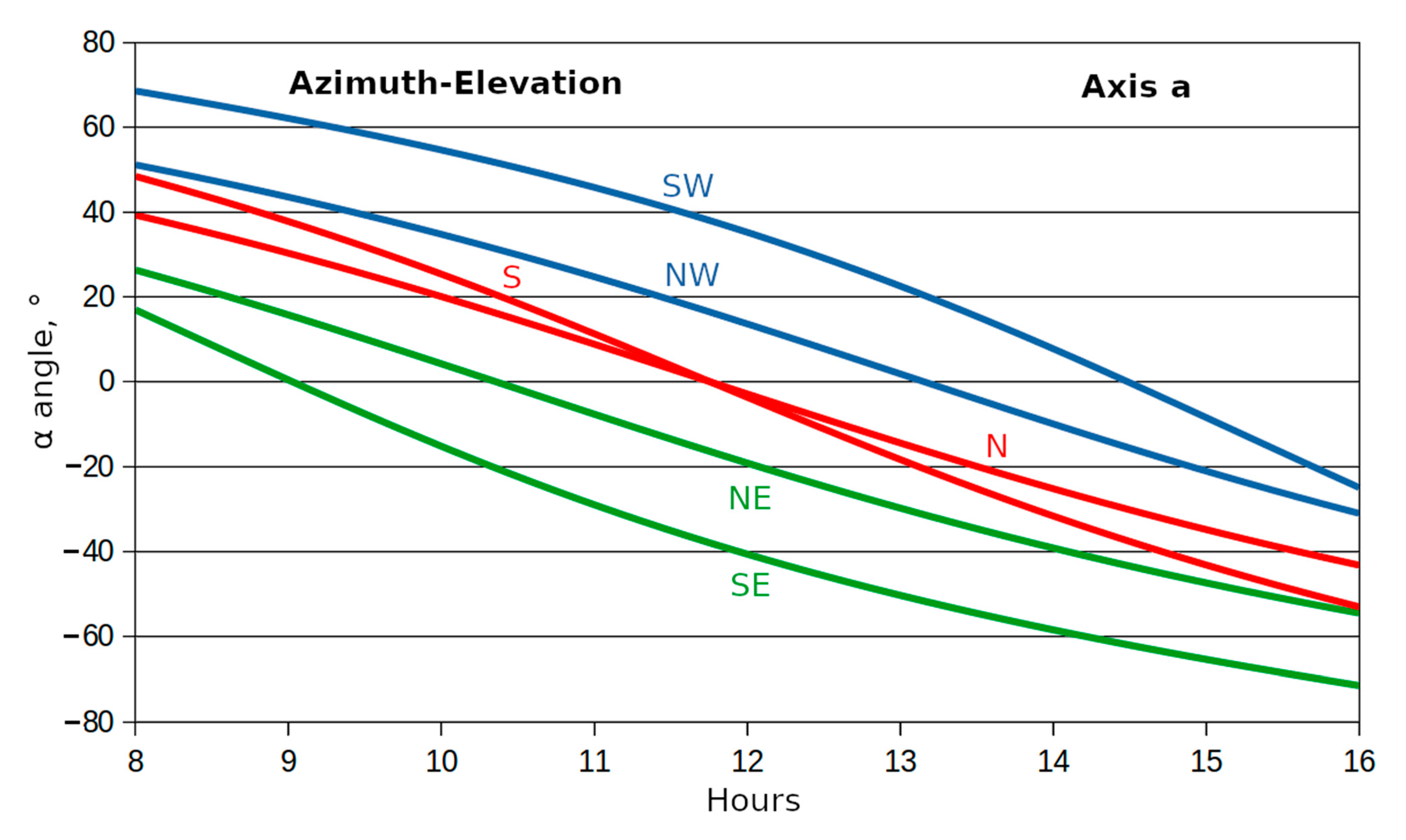
Primary axis rotation, α (in degrees), for the 6 representative heliostats (SW, S, SE, NW, N, and NE), with an azimuth-elevation model, calculated on 20 June at Protaras, from 08:00 to 16:00 LCT.
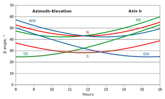
Figure 11.
Secondary axis rotation, β (in degrees), for the 6 representative heliostats (SW, S, SE, NW, N, and NE), with an azimuth-elevation model, calculated on 20 June at Protaras, from 8:00 to 16:00 LCT.

Figure 12.
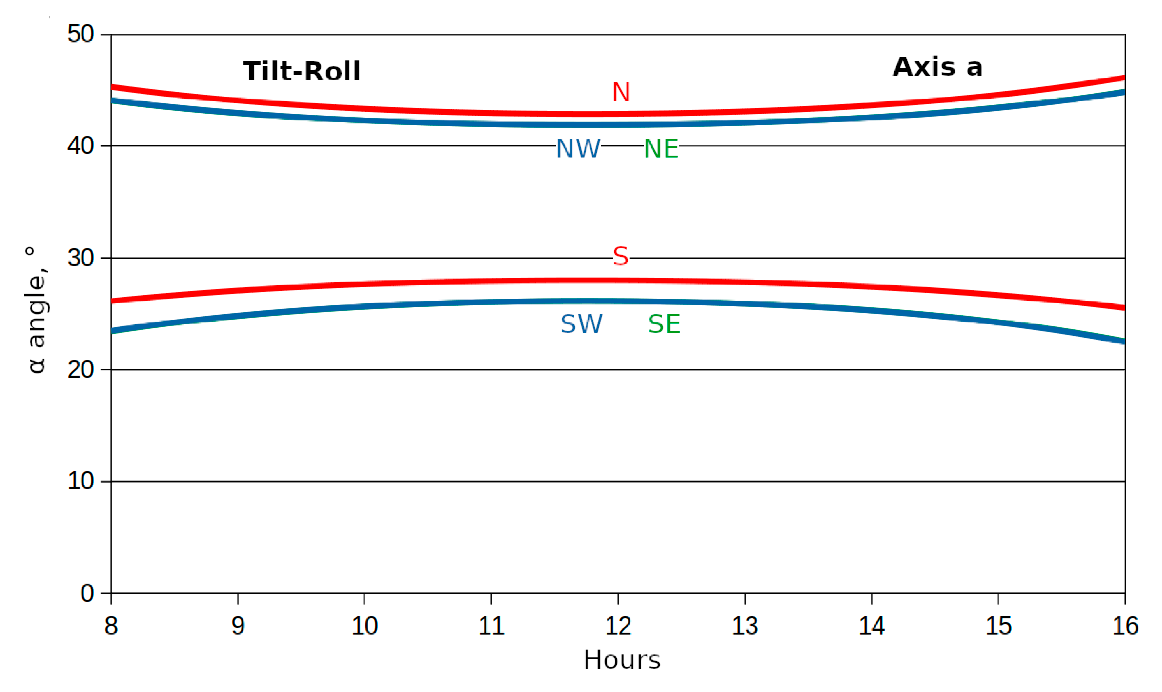
Primary axis rotation, α (in degrees), for the 6 representative heliostats (SW, S, SE, NW, N, and NE), with a tilt-roll model, calculated on 20 June at Protaras, from 8:00 to 16:00 LCT.

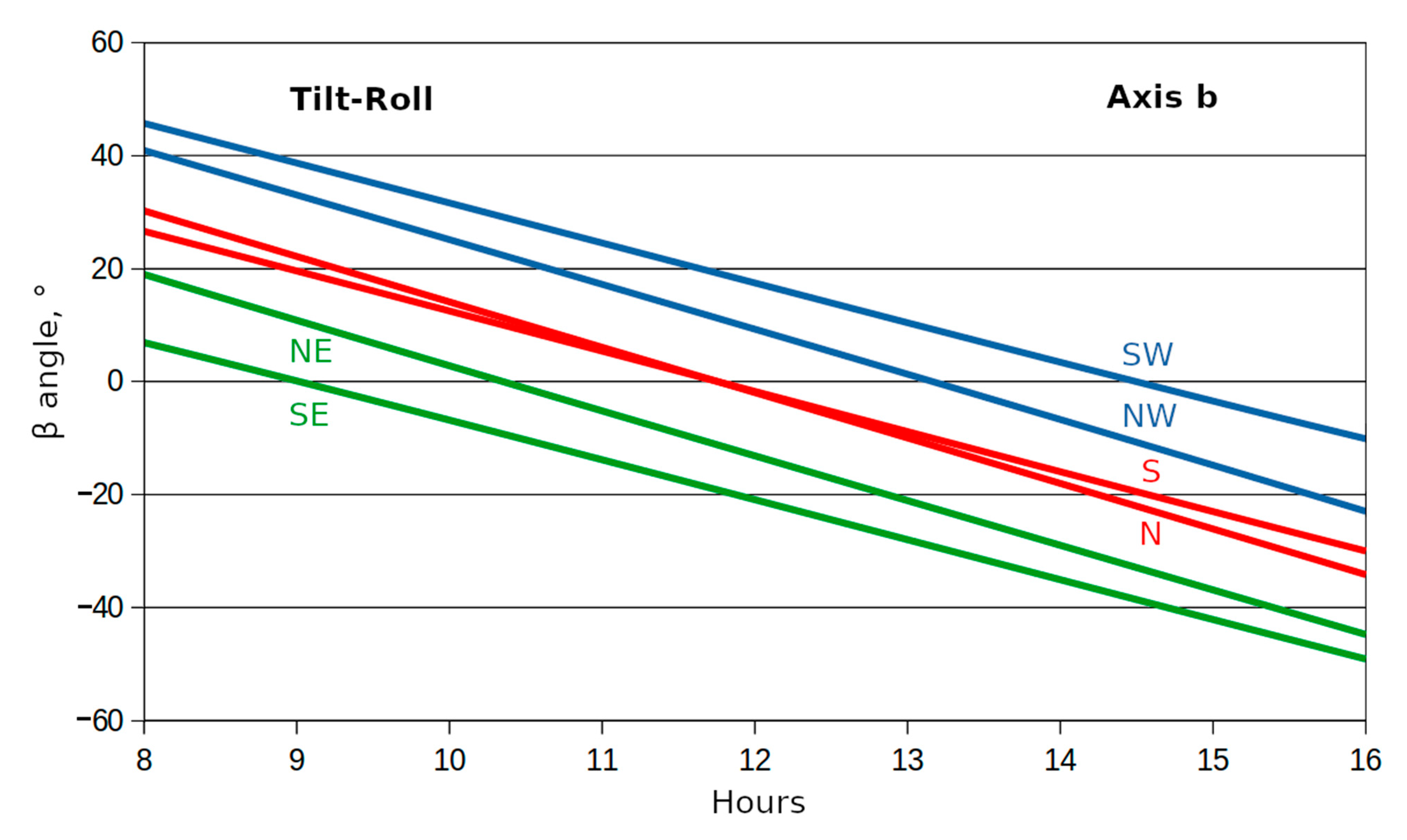
Figure 13.
Secondary axis rotation, β (in degrees), for the 6 representative heliostats (SW, S, SE, NW, N, and NE), with a tilt-roll model, calculated on 20 June at Protaras, from 8:00 to 16:00 LCT.
The heliostat curves represented in Figure 10, Figure 11, Figure 12 and Figure 13 are surprisingly symmetrical for both mechanical models, particularly for the tilt-roll. The primary axis curves for the elevation-azimuth model (Figure 10) are similar to the secondary axis curves for the tilt-roll model (Figure 13), as both essentially control the sun’s azimuth. Similarly, the secondary axis curves for the elevation-azimuth model (Figure 11) are quite similar to the primary axis curves for the tilt-roll model (Figure 12), as both essentially control the sun’s altitude.
However, even a qualitative analysis shows that the curves for the tilt-roll model are simpler, require fewer rotations, and a smaller angular range. This is evident when comparing the angular range in Figure 13 ([−50°, +50°]) with that in Figure 10 ([−70°, +70°]), and in Figure 12 ([25°, 45°]) with that in Figure 11 ([25°, 60°]). For each tilt-roll heliostat, the primary angle (controlling altitude, in Figure 12) is essentially constant during the day, while the secondary axis (controlling azimuth, in Figure 13) rotates essentially at a constant angular speed. This is the rationale behind the so-called polar-oriented single-axis heliostat. Close inspection of Figure 13 shows that this speed is about 7.5°/hour. This is the expected value, as the sun’s angular speed changes approximately 360°/24 h = 15°/hour: when the input ray is fixed and the mirror rotates δ, the reflected ray rotates 2δ. Similarly, when the input ray rotates 2δ, for the reflected ray to remain fixed, the mirror must rotate δ. Actually, the sun’s angular speed changes slightly throughout the year, as exemplified in Figure 9. For 20 June 2024, the angular speed is exactly 13.76°/hour [25], so the mirror’s angular speed should be around 13.76°/2 = 6.88°/hour. Measuring, for example, the average slope for the two red curves in Figure 13 (S, N heliostats) gives approximately 7.32°/hour. These results show that for this model, the two rotation axes are almost decoupled, and the axis a remains almost fixed throughout most of the day.
In both models, the westerly heliostats (SW, NW) require higher angles than the easterly heliostats (SE, NE) because the sun’s altitude is always lower on the westerly side at 16:00 LCT than on the easterly side at 8:00 LCT, prompting a larger effort from the SW and NW heliostats to properly align. This occurs because both Jülich (longitude = +6.3878°) and Protaras (longitude = +34.0583°) are located on the eastern side of the corresponding time zone (see [25] for details). As expected, in both models (Figure 11 and Figure 12), the southern heliostats (SW, S, SE), which are closer to the target, require smaller rotations (smaller altitude-controlling angles) to align the altitude than the northern ones (NW, N, NE).
Table 1 reports the most relevant data for the six mechanical models (see Figure 4 and Figure 5) studied in this work: (1) azimuth-elevation matrix-aligned AE; (2) azimuth-elevation radial-aligned AE/TA; (3) tilt-roll matrix-aligned TR; (4) tilt-roll radial-aligned TR/TA; (5) target-aligned with azimuth-elevation rotations TA/AE; and (6) target-aligned with tilt-roll rotations TA/TR. The table includes minimum and maximum rotation angles and total yearly rotations, averaged for the six representative heliostats studied (SW, S, SE, NW, N, and NE), for both the primary (α) and secondary (β) rotation axes for Jülich and Protaras.

Table 1.
Minimum and maximum α, β rotation angles, plus total accumulated α, β angular rotations, averaged for the 6 representative heliostats (SW, S, SE, NW, N, NE), from 1 January to 31 December 2024, with rectangular heliostats and 10° slope, for Jülich and Protaras, for the six mechanical models: AE and AE/TA, TR and TR/TA, TA/AE and TA/TR (see Section 2. Heliostat Orientation).
According to these numbers, the three tilt-roll models (TR, TR/TA, and TA/TR) require less total rotation and smaller rotation ranges than the azimuth-elevation models (AE, AE/TA, and TA/AE). This is essentially due to the rotation axis controlling azimuth (the α primary angle in AE models and the β secondary angle in TR models). The most striking difference is between the two target-aligned models, TA/AE and TA/TR, which rank respectively last and first in this mechanical rotation ranking. While TA/AE requires the whole [−180°, +180°] range to orient the heliostat, TA/TR requires only a much smaller [−47°, +52°] range. It should be mentioned that rotations are actually allowed to proceed beyond the fixed angle limits [−180°, +180°], so for example, if the angle goes from +179° to +181°, the final angle is registered as −179°, but the actual rotation, which is added to the total rotation, is recorded as only 2°.
As a consequence, TA/TR requires about 6–7 times fewer yearly rotations than TA/AE. This is mainly due to the front row heliostats (SW, S, SE), which are closer to the target and require significant rotations in winter to properly orient in the TA/AE model. TA models are seldom used due to their enormous installation and maintenance disadvantages, but these results seem to suggest that TA/TR is a very efficient mechanical rotation model, requiring much fewer yearly rotations than TR, the second-best model in this study. The ratio between the total rotations (α + β) needed by TR and TA/TR models amounts to 1.54 in Jülich and 1.41 in Protaras, suggesting that TA/TR would be particularly efficient in more adverse light conditions, as observed in Jülich.
The results reported in Table 1 for the AE/TA and TR/TA radial-aligned models are very similar (AE) or even slightly worse (TR) than those reported for the matrix-aligned AE and TR models. Given the increased complexity of these aligned models, where the y-axis is aligned with the target direction instead of simply pointing south–north, as in the matrix-aligned AE and TR models, it seems safe to conclude that they do not represent an improvement over the commonly used AE and TR models.
It is important to mention that every morning, the heliostats start from the rest orientation (α = 0, β = 0) at 08:00 LCT and return to this orientation at the end of the day, at 16:00 LCT. These parking rotations are a significant part of the total rotations performed by each heliostat during the day and therefore contribute to the total rotations reported in Table 1. In Protaras, when parking is not applied, the total annual α-β rotations decrease by 0.1–77.4% (AE), 0.1–77.4% (AE/TA), 1.4–45.4% (TA/AE), 90.3–0.1% (TR), 70.2–0.1% (TR/TA), and 29.3–0.1% (TA/TR). Clearly, parking primarily affects the axis controlling the altitude: the secondary axis, b, in azimuth-elevation models (AE, AE/TA, and TA/AE) and the primary axis, a, in tilt-roll models (TR, TR/TA, and TA/TR).
To show how the various heliostats behave throughout the year, Figure 14, Figure 15, Figure 16 and Figure 17 represent the total (α + β) daily rotation for the six representative heliostats (SW, S, SE, NW, N, and NE; see Figure 8) during the year 2024, for the azimuth-elevation (AE) and tilt-roll (TR) models (arguably the heliostat models most commonly used in research and production) in Jülich and Protaras. Although the general trends are similar for Jülich and Protaras, rotations are larger in Protaras for the AE model (Figure 14 and Figure 15). This is expected since the sun’s altitude changes significantly more in Protaras than in Jülich throughout the day, both in summer and winter (see [25]).
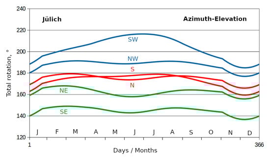
Figure 14.
Total daily rotation (in degrees), adding the two angles for primary and secondary axes, for the six representative heliostats (SW, S, SE, NW, N, and NE), calculated for the azimuth-elevation mechanical model at Jülich, for the whole year of 2024.
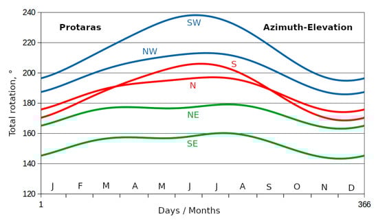
Figure 15.
Total daily rotation (in degrees), adding the two angles for primary and secondary axes, for the six representative heliostats (SW, S, SE, NW, N, and NE), calculated for the azimuth-elevation mechanical model at Protaras, for the whole year of 2024.

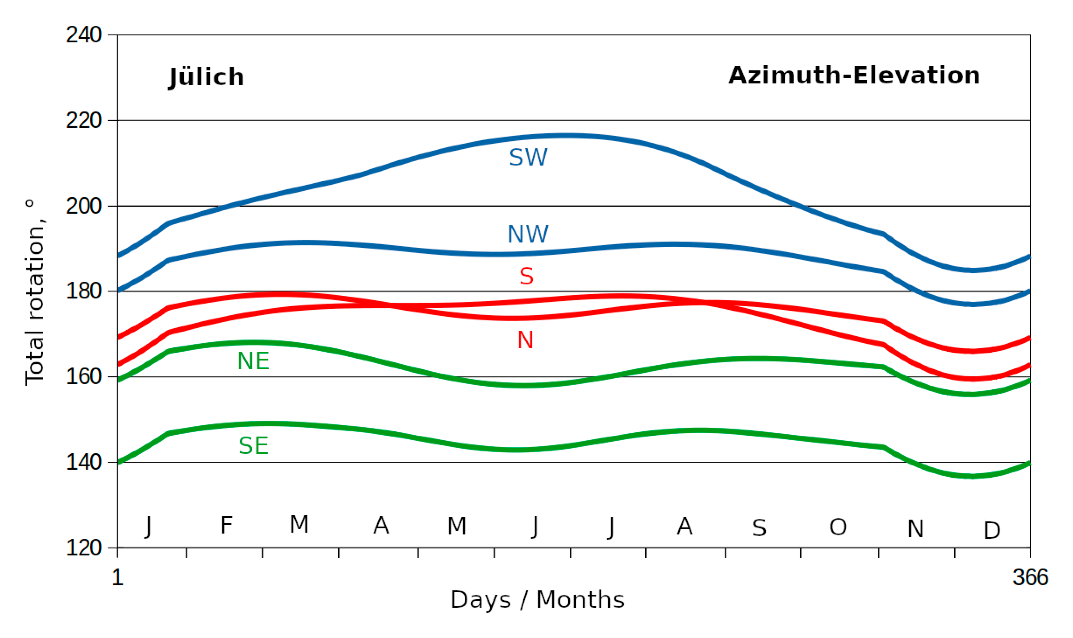
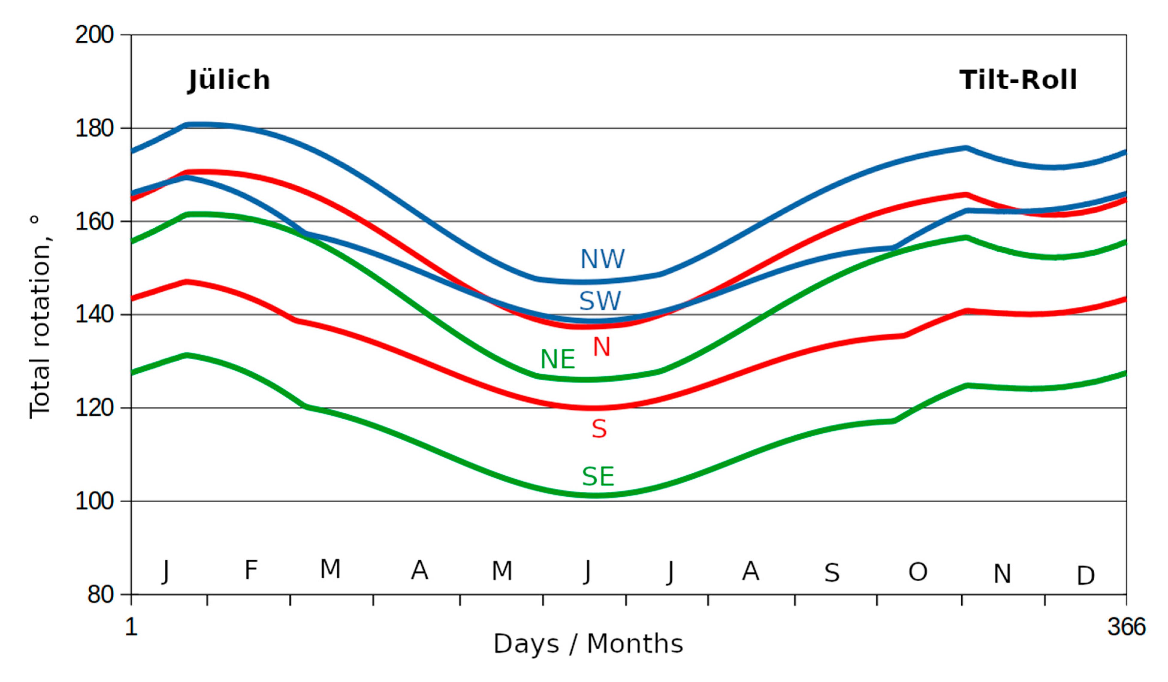
Figure 16.
Total daily rotation (in degrees), adding the two angles for primary and secondary axes, for the six representative heliostats (SW, S, SE, NW, N, and NE), calculated for the tilt-roll mechanical model at Jülich, for the whole year of 2024.

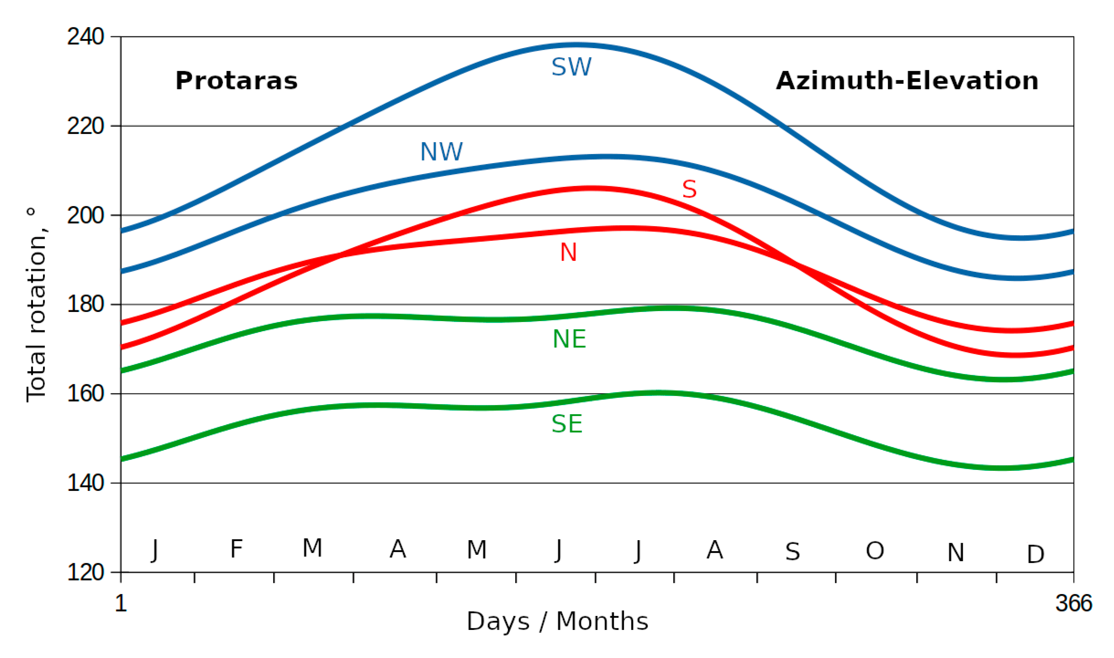
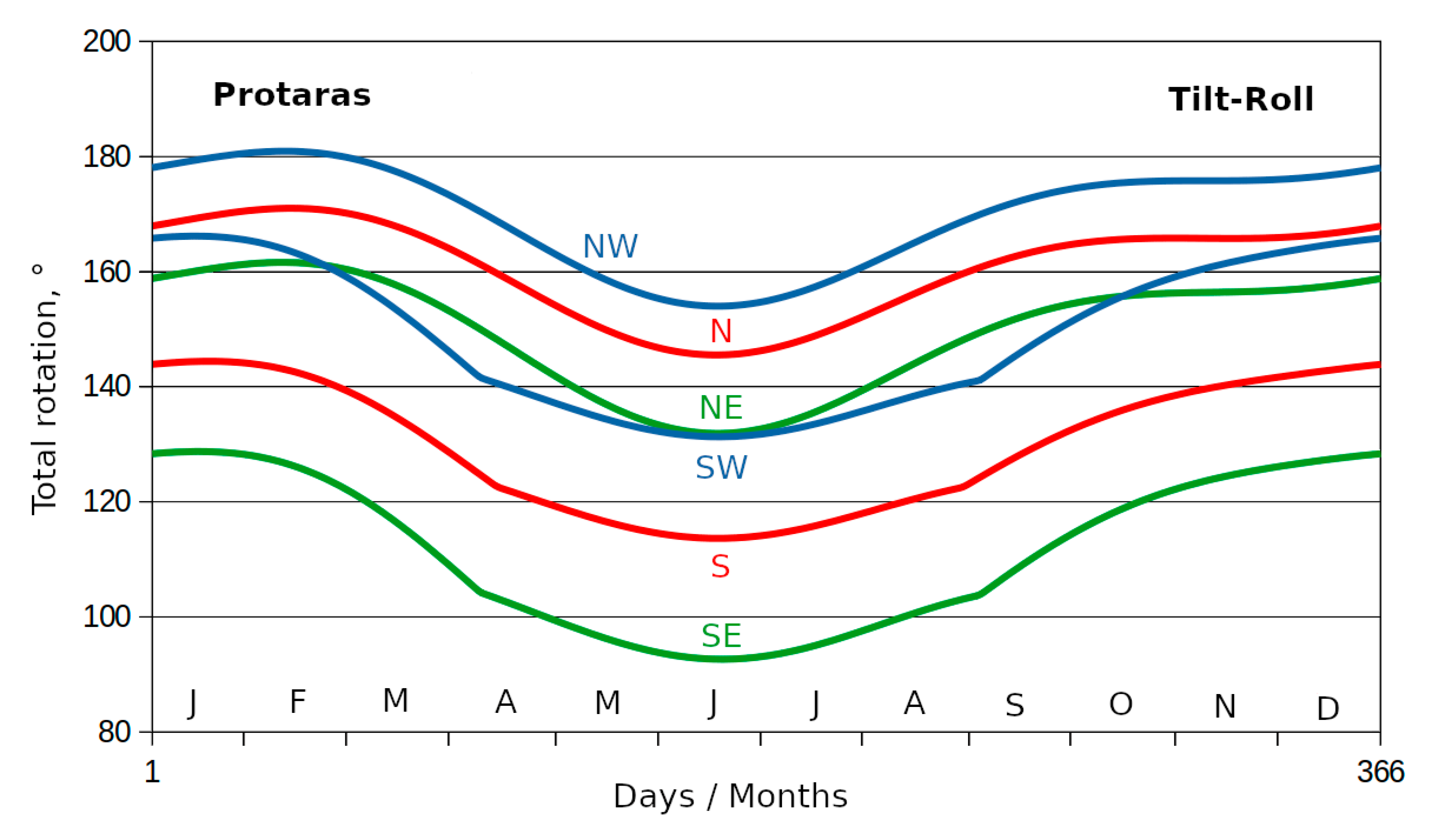
Figure 17.
Total daily rotation (in degrees), adding the two angles for primary and secondary axes, for the six representative heliostats (SW, S, SE, NW, N, and NE), calculated for the tilt-roll mechanical model at Protaras, for the whole year of 2024.
For the AE model, both Jülich and Protaras show that the westerly-oriented heliostats (SW, NW) rotate more, and the easterly-oriented heliostats (SE, NE) rotate less than the central heliostats (Figure 14 and Figure 15). As discussed above, these significant differences occur because throughout the whole year, the sun’s altitude is always lower at 16:00 LCT than at 08:00 LCT in Jülich and Protaras, due to their eastern location in the time zone [25]. Therefore, the closer westerly-oriented heliostats at 16:00 LCT require more daily rotations than the farther easterly-oriented heliostats. It is important to note that in winter, it is night at 16:00 LCT in Jülich (the sun’s altitude is negative) (see [25] for more details), so the mechanical rotations needed slightly decrease.
Daily rotations in the AE models are larger in summer, when the sun’s trajectory reaches greater ranges of altitude and azimuth (Figure 14 and Figure 15). Interestingly, the opposite occurs in the TR models because the smaller rotations needed in TR models are more affected by low Sun trajectories in winter, making orientation more difficult (Figure 16 and Figure 17).
In the TR model, both in Jülich and Protaras, the southern heliostats (SW, S, and SE), which are closer to the target, rotate less than the northern heliostats (NW, N, and NE). However, this trend is not observed in the azimuth-elevation model, where the heliostat that rotates more is the SW, and the heliostat that rotates less is the SE.
Figure 16 and Figure 17 show that in spring and autumn, the three southern heliostats (SW, S, and SE) in the TR model experience a sudden slight increase in total rotation (α + β) toward the winter direction, which is almost discontinuous. This increase is only due to the primary angle α (which controls altitude) and occurs around 4 March and 5 October in Jülich and around 8 April and 5 September in Protaras. These dates are not associated with any notable astronomical dates for Jülich or Protaras [25].
7.2. Mechanical Rotation Issues
Close inspection of Table 1 shows some interesting results. Models AE and AE/TA show exactly the same yearly total rotations. These models differ only in the azimuth (α) angle, so this equality was expected for the altitude (β) angle. However, detailed software testing shows that the total α rotations (updating every 30 s) for a workday (from 08:00 to 16:00 LCT) across all 366 days of 2024 are exactly equal for the AE and AE/TA models (within six decimal places), as differences in the morning are compensated for in the afternoon. The small difference observed for Jülich in Table 1 is due to the fact that it is night at 16:00 LCT in winter (from 3 November to 21 January), so no rotations occur at that time, resulting in a break in the daily symmetry.
For 30 s at Jülich (31 March 2024 at 09:11 LCT) and 60 s at Protaras (28 February 2024 at 09:26 and 09:27 LCT), the model TA/AE is unable to align the SW heliostat (see Figure 8). No such misfit was registered for any other heliostat or mechanical model during the whole year. This occurs because at these precise moments, the β angle tends to 0°. At Protaras, as time progresses, β keeps decreasing until it reaches 0.152°, then the misfit occurs, and then β starts increasing again, starting from 0.044°. In Jülich, β keeps decreasing until it reaches 0.084° and stops aligning, and then β starts increasing again, starting from 0.193°. In the AE and AE/TA models, this problem cannot happen because an aligned heliostat cannot point to the sky (β = 0°). However, in the TA/AE model, this is possible when the sun is exactly at the target position as seen from the heliostat (when the vector sun, , and the vector target, , are aligned; see Figure 4a). Admittedly, this misfit is partially due to the very strict convergence criterion used throughout this work: both the α and β angles must converge to less than 10−10 rad in fewer than 1000 iterations for the mirror orientation task to be successfully accepted. Easing the convergence criterion to 10−9 rad resolves the problem (for the time instances mentioned above, the β angle becomes 0.135° at Jülich and 0.093° and 0.038° at Protaras). Increasing the number of iterations, even to 100 000, does not resolve the problem.
In all azimuth-elevation models (AE, AE/TA, and TA/AE), it is assumed that the β angle ranges from 0° to some positive value, usually not exceeding 90° (corresponding to the polar angle in spherical coordinates). In AE and AE/TA models, this angle cannot be negative; otherwise, the heliostat would be pointing away from the target. In the TA/AE model, when the sun is above the target (in summer, around 12:00 LCT), the heliostat needs to rotate upward, making the β angle positive (the x-axis points westerly; see Equation (6) and Figure 4a), and relatively small α rotation angles are needed to achieve the required orientation. However, when the Sun is below the target center (in winter, around 08:00 and 16:00 LCT), the heliostat needs to rotate downwards, resulting in a negative β angle. As the β angle is always assumed to be positive (as if the mechanical axis only rotates to one side), the α angle needs to rotate close to 180° to meet the required orientation. This is why the α angle needs to rotate so widely in this TA/AE model, from −180° to +180°. This problem affects the front row heliostats more (see the working range required for the α angle with the TA/AE model in Table 2), as they are more prone to see the sun below the target (see Figure 18). At Protaras, the α angle in the back row heliostats ranges only from −93.02° to +100.81° (still a large range) throughout the whole year. The land slope of 10° used throughout this work (see Section 5, Computational Details) also increases the height of the back row heliostats, emphasizing these differences in the α angles.
Table 2.
Minimum and maximum α angles for the TA/AE model, for Jülich and Protaras, and for the six representative heliostats: SW, S, SE, NW, N, and NE (see Figure 8). The angular range is larger for the front row and for Jülich.
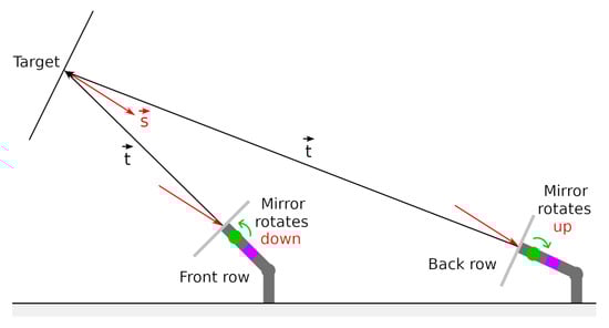
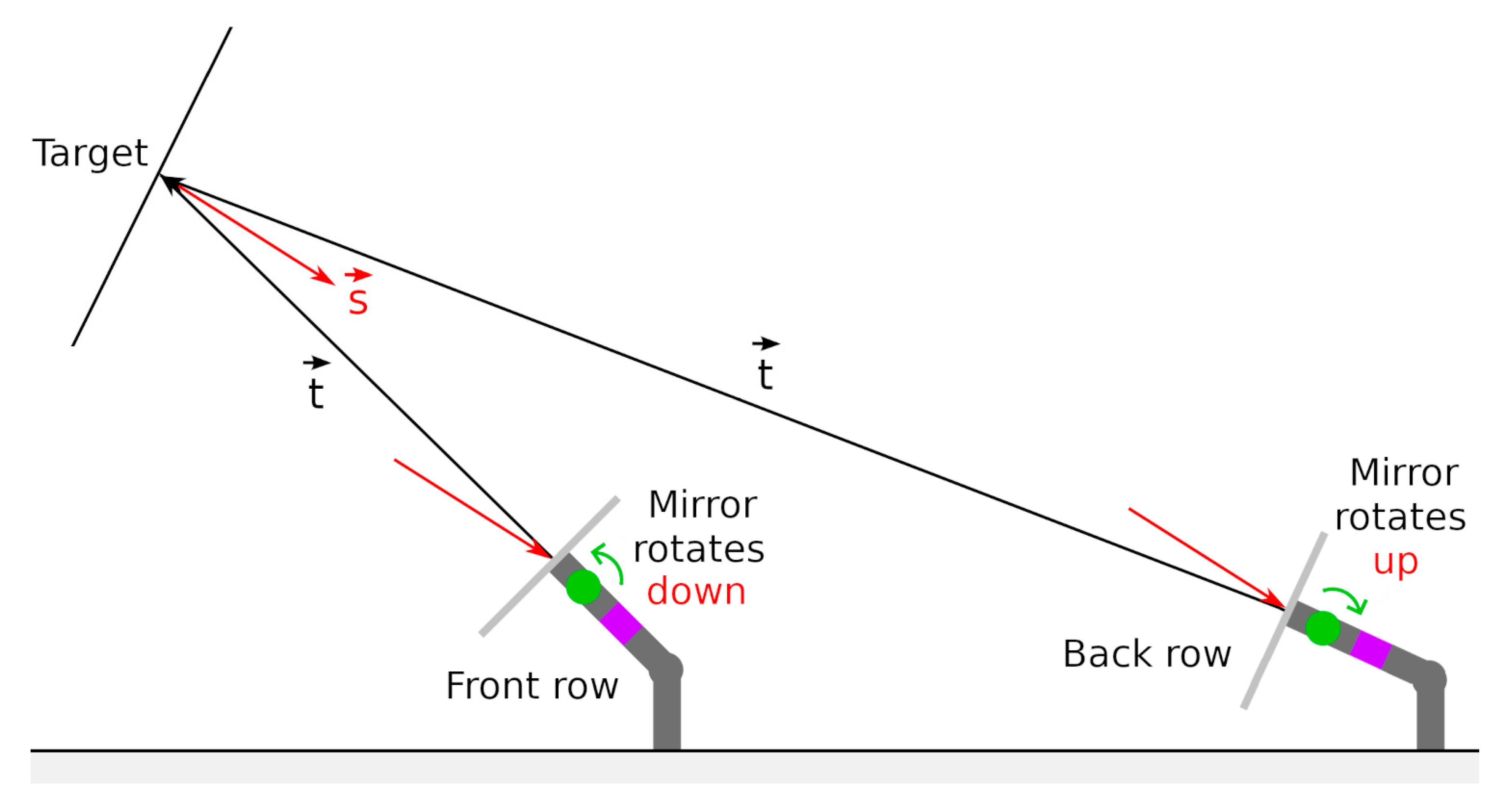
Figure 18.
For simplicity, it is assumed that this image represents the heliostat field for TA/AE model when daily working period starts (at 08:00 LCT in our simulations). Initially, all heliostats are at parking orientation (α = β = 0°), with the mirrors pointing to the target (defined by vector ). The front row heliostats see the Sun (defined by vector ) below the target, so they must rotate down (β < 0°) to align. The back row heliostats see the Sun above the target, so they must rotate up (β > 0°) to align. The land slope is set to 0° for simplicity.
As expected, these issues work differently in the TA/TR model. At Protaras on 28 February 2024, both α and β angles change from negative to positive values around 09:27 LCT (for heliostat S, see Figure 8), where the two angles reach a combined minimum, with α = 0.006° and β = −0.038°. At Jülich on 31 March 2024, both α and β angles again change from negative to positive values around 09:12 LCT (also for heliostat S), reaching a combined minimum with α = 0.004° and β = 0.135°. At both instances, the Sun is exactly aligned with the target (as seen from heliostat S), the model performs well, and the flux radiation image collected at the target is accurate. The angular range needed to align the six heliostats (see Table 3) throughout the whole year is surprisingly small for both α and β angles: [−16.89°, 46.79°] and [−46.62°, 51.87°], respectively (see Table 1). Again, the front row heliostats require more negative α angles than the back row heliostats (see the working range required for the α angle, with the TA/TR model, in Table 3).
Table 3.
Minimum and maximum α angles for the TA/TR model, for Jülich and Protaras, and for the six representative heliostats: SW, S, SE, NW, N, and NE (see Figure 8). α Min is more negative for the front row and for Jülich.
The issues described above for the TA/AE model could be solved, for example, using the following two approaches: (1) every time the α angle is outside the [−90°, 90°] range (likely because the β angle is negative, necessitating a large α rotation), the direction of the β rotation could be inverted (inverting the axis b); (2) the initial (parking) angle β = 0° could be redefined to point to the sky instead of pointing to the target, ensuring that the β angle is always positive (with the x-axis pointing easterly, as in the other azimuth-elevation models). The usefulness of these solutions may be questioned, however, considering that they require more complex mechanical systems, the other target-aligned model (TA/TR) operates well, and target-aligned models are seldom used anyway due to their complex implementation.
8. Conclusions
- (1)
- The heliostats’ orientation must be updated at least once a minute to adequately follow the sun’s trajectory.
- (2)
- The daily rotation curves are quite symmetrical for both the primary and secondary axes, as well as for the azimuth-elevation and tilt-roll models.
- (3)
- In azimuth-elevation models, the primary axis controls azimuth, and the secondary axis controls altitude. In tilt-roll models, the primary axis controls altitude, and the secondary axis controls azimuth.
- (4)
- The daily rotation curves are strikingly similar in both the azimuth-elevation and tilt-roll models, for the axes controlling azimuth and the axes controlling altitude.
- (5)
- Tilt-roll models are more efficient than azimuth-elevation models, requiring smaller angular ranges and smaller angular rotations throughout a full working year, every day from 08:00 to 16:00 LCT.
- (6)
- When the daily working period is defined without taking into account the local longitude, westerly and easterly heliostats require different rotations, even when symmetrically located in the heliostat field.
- (7)
- Front and back row heliostats have significantly different mechanical requirements. Front heliostats are notoriously more difficult to orient in TA/AE models, particularly at low sun altitudes (in the morning, during winter, at high latitudes).
- (8)
- The yearly rotation curves indicate that to achieve orientation, azimuth-elevation heliostats rotate more in summer, while tilt-roll heliostats rotate more in winter.
- (9)
- Axial-based azimuth-elevation and tilt-roll models exhibit similar performance to that of the (more complex) equivalent radial-based models.
- (10)
- Target-aligned models with tilt-roll rotations work better than the tilt-roll model. Target-aligned models with azimuth-elevation rotations perform worse than the azimuth-elevation model. In the limit, target-aligned models with azimuth-elevation rotations might be vulnerable to numerical inaccuracies.
- (11)
- Parking heliostats at the end of each working day significantly increases the total mechanical rotations for the axis controlling altitude in both azimuth-elevation and tilt-roll models.
The wide range of significant conclusions achieved in this work shows that accurate computer modeling of large solar facilities is essential for improving our knowledge of the mechanical (and optical) aspects involved, decreasing costs, and maximizing economic efficiency.
Author Contributions
J.C.G.P., conceptualization, methodology, software, data curation, validation, and writing—original draft preparation. L.G.R., formal analysis, validation, writing—review and editing, project administration, and funding acquisition. All authors have read and agreed to the published version of the manuscript.
Funding
This work benefited from financial support from the European Union through the SFERA-III project, Grant Agreement No. 823802 (proposal SURPF2101310018-CAHO “Development of Computer Algorithms to Optimize Heliostat Orientation”). The authors would like to thank the Fundação para a Ciência e a Tecnologia (FCT) for its financial support through the LAETA Base Funding (DOI: 10.54499/UIDB/50022/2020).
Institutional Review Board Statement
Not applicable.
Informed Consent Statement
Not applicable.
Data Availability Statement
The software source code and data supporting the conclusions of this article will be made available by the authors on request.
Acknowledgments
The authors would like to thank The Cyprus Institute for providing access to its installations and for the support of its scientific and technical staff in 2022, as part of the European Union SFERA-III project (Grant Agreement No. 823802).
Conflicts of Interest
The authors declare no conflicts of interest.
Abbreviations
The following abbreviations are used in this manuscript:
| AE | Azimuth-elevation |
| AE/TA | Azimuth-elevation, radial-aligned with target |
| Heliostat center vector | |
| CSP | Concentrating solar power |
| Unit incident sun vector in the horizontal referential | |
| LCT | Local time |
| Unit normal vector | |
| o1 | Offset 1 (distance between axis a and axis b) |
| o2 | Offset 2 (distance between axis b and mirror) |
| Ray position in the horizontal referential | |
| Ray position in the original real referential | |
| Unit reflected sun vector in the horizontal referential | |
| Unit sun vector | |
| Target vector | |
| TA | Target-aligned |
| TA/AE | Target-aligned, with azimuth-elevation rotations |
| TA/TR | Target-aligned, with tilt-roll rotations |
| TR | Tilt-roll |
| TR/TA | Tilt-roll, radial-aligned with target |
| α | Angle corresponding to axis a (primary axis) |
| β | Angle corresponding to axis b (secondary axis) |
| δ | Angle that the target plane makes with the vertical direction |
| Polar angle (in spherical coordinates) | |
| Azimuth angle (in spherical coordinates) |
References
- Cocco, D.; Petrollese, M.; Tola, V. Exergy analysis of concentrating solar systems for heat and power production. Energy 2017, 130, 192–203. [Google Scholar] [CrossRef]
- Bellos, E. Progress in beam-down solar concentrating systems. Prog. Energy Combust. Sci. 2023, 97, 101085. [Google Scholar] [CrossRef]
- Alexopoulos, S.; Hoffschmidt, B. Concentrating Receiver Systems (Solar Power Tower). In Encyclopedia of Sustainability Science and Technology; Meyers, R.A., Ed.; Springer: New York, NY, USA, 2012; pp. 2349–2391. [Google Scholar] [CrossRef]
- Hughes, G. A solar furnace using a horizontal heliostat array. Sol. Energy 1958, 2, 49–51. [Google Scholar] [CrossRef]
- Mills, D. Was the Italian solar energy pioneer Giovanni Francia right? Areva Sol. 2013, 15, 1–13. Available online: https://www.gses.it/incontri/8luglio2013/MillsPaper08.07.2013.pdf (accessed on 18 February 2025).
- Global Energy Observatory: PS10 Solar Power Plant Spain. Available online: https://globalenergyobservatory.org/geoid/4942 (accessed on 18 February 2025).
- The World’s First Baseload (24/7) Solar Power Plant. Available online: https://www.forbes.com/sites/tonyseba/2011/06/21/the-worlds-first-baseload-247-solar-power-plant/ (accessed on 18 February 2025).
- Eddhibi, F.; Amara, M.B.; Balghouthi, M.; Guizani, A.A. Design and analysis of a heliostat field layout with reduced shading effect in southern Tunisia. Int. J. Hydrogen Energy 2017, 42, 28973–28996. [Google Scholar] [CrossRef]
- Deng, H.; Chen, H.; Wang, X. Design of heliostat field based on ray tracing. Highlights Sci. Eng. Technol. 2024, 87, 10–16. [Google Scholar] [CrossRef]
- Ortega, G.; Barbero, R.; Rovira, A. Global methods for calculating shading and blocking efficiency in central receiver systems. Energies 2024, 17, 1282. [Google Scholar] [CrossRef]
- Leonardi, E.; Pisani, L. Analysis of heliostats’ rotation around the normal axis for solar tower field optimization. J. Sol. Energy Eng. 2016, 138, 031007. [Google Scholar] [CrossRef]
- Waghmare, S.A.; Puranik, B.P. Analysis of tracking characteristics of a heliostat field using a graphical ray tracing procedure. e-Prime—Adv. Electr. Eng. Electron. Energy 2023, 6, 100354. [Google Scholar] [CrossRef]
- Martínez-Hernández, A.; Gonzalo, I.B.; Romero, M.; Gonzalez-Aguilar, J. Experimental and numerical evaluation of drift errors in a solar tower facility with tilt-roll tracking-based heliostats. AIP Conf. Proc. 2020, 2303, 030026. [Google Scholar] [CrossRef]
- Martínez-Hernández, A.; Gonzalo, I.B.; Romero, M.; Gonzalez-Aguilar, J. Drift analysis in tilt-roll heliostats. Sol. Energy 2020, 211, 1170–1183. [Google Scholar] [CrossRef]
- Lewen, J.; Pargmann, M.; Cherti, M.; Jitsev, J.; Pitz-Paal, R.; Quinto, D.M. Inverse Deep Learning Raytracing for heliostat surface prediction. Sol. Energy 2025, 289, 113312. [Google Scholar] [CrossRef]
- Vazquez, E.; Martínez-Hernandez, A.; Jamil, B.; Prodanovic, M.; González-Aguilar, J.; Romero, M. Pointing correction based on limit cycles oscillators applied on a heliostats field digital twin. Sustain. Energy Technol. Assess. 2024, 68, 103849. [Google Scholar] [CrossRef]
- Pereira, J.C.G.; Rosa, L.G. Computer modelling of heliostat fields by ray-tracing techniques: Simulating shading and blocking effects. Appl. Sci. 2025, 15, 2953. [Google Scholar] [CrossRef]
- Tonatiuh, a Monte Carlo Ray Tracer for the Optical Simulation of Solar Concentrating Systems. Available online: https://iat-cener.github.io/tonatiuh/ (accessed on 24 February 2025).
- NREL SolTrace. Available online: https://www2.nrel.gov/csp/soltrace (accessed on 24 February 2025).
- Photon Engineering. What Is FRED? Available online: https://photonengr.com/fred (accessed on 24 February 2025).
- Ansys Zemax OpticStudio Comprehensive Optical Design Software. Available online: https://www.ansys.com/products/optics/ansys-zemax-opticstudio (accessed on 24 February 2025).
- Synopsys CODE V Optical Design Software. Available online: https://www.synopsys.com/optical-solutions/codev.html (accessed on 24 February 2025).
- Synopsys LightTools Illumination Design Software. Available online: https://www.synopsys.com/optical-solutions/lighttools.html (accessed on 24 February 2025).
- Lambda Research Corporation TracePro Software for Design and Analysis of Illumination and Optical Systems. Available online: https://lambdares.com/tracepro (accessed on 24 February 2025).
- Pereira, J.C.G.; Domingos, G.; Rosa, L.G. Computer modelling of heliostat fields by ray-tracing techniques: Simulating the Sun. Appl. Sci. 2025, 15, 1739. [Google Scholar] [CrossRef]
- Romero, M.; González-Aguilar, J.; Luque, S. Ultra-modular 500m2 heliostat field for high flux/high temperature solar-driven processes. AIP Conf. Proc. 2017, 1850, 030044. [Google Scholar] [CrossRef]
- Pereira, J.C.G.; Fernandes, J.C.; Guerra Rosa, L. Mathematical models for simulation and optimization of high-flux solar furnaces. Math. Comput. Appl. 2019, 24, 65. [Google Scholar] [CrossRef]
- Pereira, J.C.G.; Rodríguez, J.; Fernandes, J.C.; Rosa, L.G. Homogeneous flux distribution in high-flux solar furnaces. Energies 2020, 13, 433. [Google Scholar] [CrossRef]
- Pereira, J.C.G.; Rahmani, K.; Rosa, L.G. Computer modelling of the optical behavior of homogenizers in high-flux solar furnaces. Energies 2021, 14, 1828. [Google Scholar] [CrossRef]
- EU SFERA-III Project. Available online: https://sfera3.sollab.eu/access/#infrastructures (accessed on 24 February 2025).

Disclaimer/Publisher’s Note: The statements, opinions and data contained in all publications are solely those of the individual author(s) and contributor(s) and not of MDPI and/or the editor(s). MDPI and/or the editor(s) disclaim responsibility for any injury to people or property resulting from any ideas, methods, instructions or products referred to in the content. |
© 2025 by the authors. Licensee MDPI, Basel, Switzerland. This article is an open access article distributed under the terms and conditions of the Creative Commons Attribution (CC BY) license (https://creativecommons.org/licenses/by/4.0/).