Article

Modified Grey Wolf Optimizer and Application in Parameter Optimization of PI Controller

1
The College of Artificial Intelligence, China University of Petroleum (Beijing), Beijing 102249, China
2
The College of Engineer, China University of Petroleum (Beijing) at Karamay, Karamay 834099, China
*
Author to whom correspondence should be addressed.
Appl. Sci. 2025, 15(8), 4530; https://doi.org/10.3390/app15084530
Submission received: 24 March 2025 / Revised: 10 April 2025 / Accepted: 16 April 2025 / Published: 19 April 2025
(This article belongs to the Section Computing and Artificial Intelligence)

Abstract

:

Featured Application

The M-GWO has excellent optimization ability for benchmark functions and potential engineering problem-solving ability.

Abstract

The Grey Wolf Optimizer (GWO) is a well-known metaheuristic algorithm that currently has an extremely wide range of applications. However, with the increasing demand for accuracy, its shortcomings of low exploratory and population diversity are increasingly exposed. A modified Grey Wolf Optimizer (M-GWO) is proposed to tackle these weaknesses of the GWO. The M-GWO introduces mutation operators and different location-update strategies, achieving a balance between exploration and development. The experiment validated the performance of the M-GWO using the CEC2017 benchmark function and compared the results with five other advanced metaheuristic algorithms: the Improved Grey Wolf Optimizer (IGWO), GWO, Whale Optimization Algorithm (WOA), Dung Beetle Optimizer (DBO), and Harris Hawks Optimization (HHO). The performance results indicate that the M-GWO has a better performance than competitor algorithms on all 29 functions in dimensions 30 and 50, except for function 26 in dimension 30 and function 28 in dimension 50. Compared with competitor algorithms, the proposed M-GWO is the most effective algorithm, with an overall effectiveness of 96.5%. In addition, in order to show the value of the M-GWO in the practical engineering field, the M-GWO is used to optimize the PI controller parameters of the current loop of the permanent magnet synchronous motor (PMSM) system. By designing a PI controller parameter optimization scheme based on the M-GWO, the fluctuation of the q-axis current and d-axis current of the motor is reduced. The designed scheme reduces the q-axis fluctuation to around −2~1 A and the d-axis current fluctuation to around −2~2 A. By comparing the current-tracking errors of the q -axis and d -axis under different algorithms, the validity of the optimized parameters of the M-GWO is proved.

1. Introduction

Group-based metaheuristic solutions are widely recognized for their extensive applications in modern optimization tasks. Within these solutions, the search process is inherently collective. Algorithms are typically capped at a maximum number of iterations, beyond which they cease, having diligently sought the optimal solution for the group. Throughout these iterations, each participant within the group engages in ongoing searches, sharing pertinent information with peers to meet the defined objectives. This cooperative approach sets group-based metaheuristic solutions apart from their individual-based counterparts, as it facilitates a more effective search for optimal solutions.
At present, several intelligent optimization algorithms have garnered significant attention in the field of computational intelligence. The popular intelligent optimization algorithms are the Grey Wolf Optimizer (GWO) [1], particle swarm optimization (PSO) [2] algorithm, Ant Lion optimization algorithm (ALO) [3], and Dragonfly algorithm (DA) [4]. These optimization algorithms have been integrated with a diverse array of problems, demonstrating their applicability across various domains. Among these algorithms, the Grey Wolf Optimization (GWO) algorithm, a member of the swarm intelligence optimization algorithms, has garnered substantial scholarly interest due to its rapid convergence and effective optimization capabilities. However, the traditional GWO is prone to converging prematurely at local minima, a limitation that has spurred significant advancements in its enhancement. Concurrently, these improvements have yielded innovative insights and approaches to address this challenge. In [5], GWO is integrated with SCA to improve global search capability by incorporating SCA into the position update of alpha wolves in GWO. GWO has been integrated with differential algorithm (DE) to obtain DE-GWO to solve the problem of gas emission localization [6]. In [7], Gaussian mutation and spiral function are introduced to help GWO skip local optima and improve the accuracy of the algorithm. In [8], random dynamic weight allocation is introduced to the first three wolves to accelerate the convergence in the later stage of optimization, which helps to find the global optimal solution. In [9], GWO is combined with WOA, and random control parameters and dynamic weighting strategies are added to improve the convergence accuracy and speed of the algorithm. In [10], the Contact List Mechanism (CLM) is utilized to update the population and improve its diversity and convergence accuracy. Scholars have introduced a chaos grouping mechanism into GWO to improve population diversity and utilized a dynamic sufficiency mechanism to balance exploration and development [11]. In [12], a new anti-learning strategy of following control was introduced into GWO to balance global optimization and local exploration. In [13], GWO is combined with the Cuckoo search (CS) algorithm to form a fractional order algorithm model to improve algorithm accuracy and optimize the management of wireless communication systems. In [14], the adaptive multi-objective particle swarm algorithm is integrated with GWO to improve the convergence accuracy of the algorithm for predicting and optimizing intelligent environmental control systems. In [15], the ReliefF algorithm and Coupla entropy are introduced in the initialization process of GWO, and competitive guidance strategy and differential evolution-based leader wolf strategy are proposed to prevent the algorithm from becoming stuck in local optimal solutions.
Nowadays, there are numerous solutions to engineering problems using metaheuristic algorithms. However, there is still limited research on optimizing the parameters of PI/PID controllers. The traditional method will bring huge computational burden to the optimization of PI/PID controller parameters. The strong optimization ability of metaheuristic algorithms has great application prospects in the optimization of PI/PID controller parameters. In [16], GWO was used to optimize the PID controller parameters for vehicle speed and yaw rate, improving the tracking speed of the tracked vehicle for vehicle speed and yaw rate under pivot steering conditions. In [17], GWO and Teaching-Learning-Based Optimization (TLBO) algorithms were jointly optimized for PID parameters of hybrid renewable energy and evaluated through different performance functions. In [18], GWO is used to find the optimal PD controller gain in drone flight control, making the time-domain results and actuator outputs smoother. Some scholars have used the improved GWO to optimize the PID controller gain for controlling the grid frequency in a single-zone power system. The experimental results show that compared to other algorithms, the improved GWO can find the optimal PID controller gain [19]. In [20], GWO is used to optimize the PID controller parameters of a laboratory scale magnetic levitation system to eliminate nonlinear problems and instability in the system. However, in the current era of computer development, the problems of premature convergence and insufficient accuracy of GWO are becoming increasingly apparent. It is very important to improve the convergence accuracy of GWO.
To solve these weaknesses of GWO, a modified Grey Wolf Optimizer (M-GWO) is proposed. This research is based on proposing improvements to the position formula of individuals within the population of the existing Grey Wolf Optimizer (GWO) algorithm. The aim is to optimize and enhance the existing GWO algorithm to improve its optimization capabilities. The M-GWO introduces an innovative search strategy that integrates sine, cosine, Gaussian, and Cauchy mutation operators to enhance the search capabilities and diversity of the Grey Wolf population. This approach enriches the algorithm’s ability to explore the solution space more effectively. Specifically, in the location update strategy, the sine and cosine update methods are employed to refine the position of the α wolves, which are the individuals with the highest fitness, thereby facilitating more efficient local searches. Additionally, the Gaussian and Cauchy mutation operators are incorporated into the position update strategy for the ω wolves, targeting individual mutation. The influence of these mutation operators escalates with the progression of iterations, endowing the M-GWO with an enhanced capacity for global exploration.
The performance of M-GWO is developed and evaluated using the CEC2017 benchmark function [21], and the effectiveness of M-GWO is verified by comparing different algorithms. The CEC2017 benchmark functions have different types of functions, which can evaluate the exploration and development capabilities of algorithms from multiple perspectives. To better demonstrate the effectiveness of M-GWO, it is compared with some highly advanced metaheuristic algorithms currently available: Improved Grey Wolf Optimizer (IGWO) [22], GWO, Whale Optimization Algorithm (WOA) [23], Dung Beetle Optimizer (DBO) [24], and Harris Hawks Optimization (HHO) [25]. The experimental results from benchmark function tests demonstrate that the Modified Grey Wolf Optimizer (M-GWO) outperforms other algorithms in terms of effectiveness. With the exception of function 26 in 30 dimensions and function 28 in 50 dimensions, the test results of the M-GWO are superior to other algorithms. Compared to other algorithms, the M-GWO has better exploration and development capabilities. Subsequently, the designed M-GWO was used to optimize the PI controller parameters of the PMSM system current loop and compared with WOA and HHO. The experimental results demonstrate that the parameter optimization scheme of the PI controller based on the M-GWO can find the optimal PI parameters.
In the rest of this paper, firstly, Section 2 introduces the Grey Wolf Optimization algorithm and mutation operator, providing a theoretical basis for improving the Grey Wolf Optimization algorithm. Section 3 improves the Grey Wolf Optimization algorithm and introduces the theoretical advantages of the improved algorithm. In Section 4, the proposed M-GWO is tested on CEC2017 and compared with different algorithms. Subsequently, the proposed M-GWO is used to optimize the PI controller parameters of the current loop in the PMSM system and is validated through the current response curve. In Section 5, a summary of the article is provided.

2. Related Works

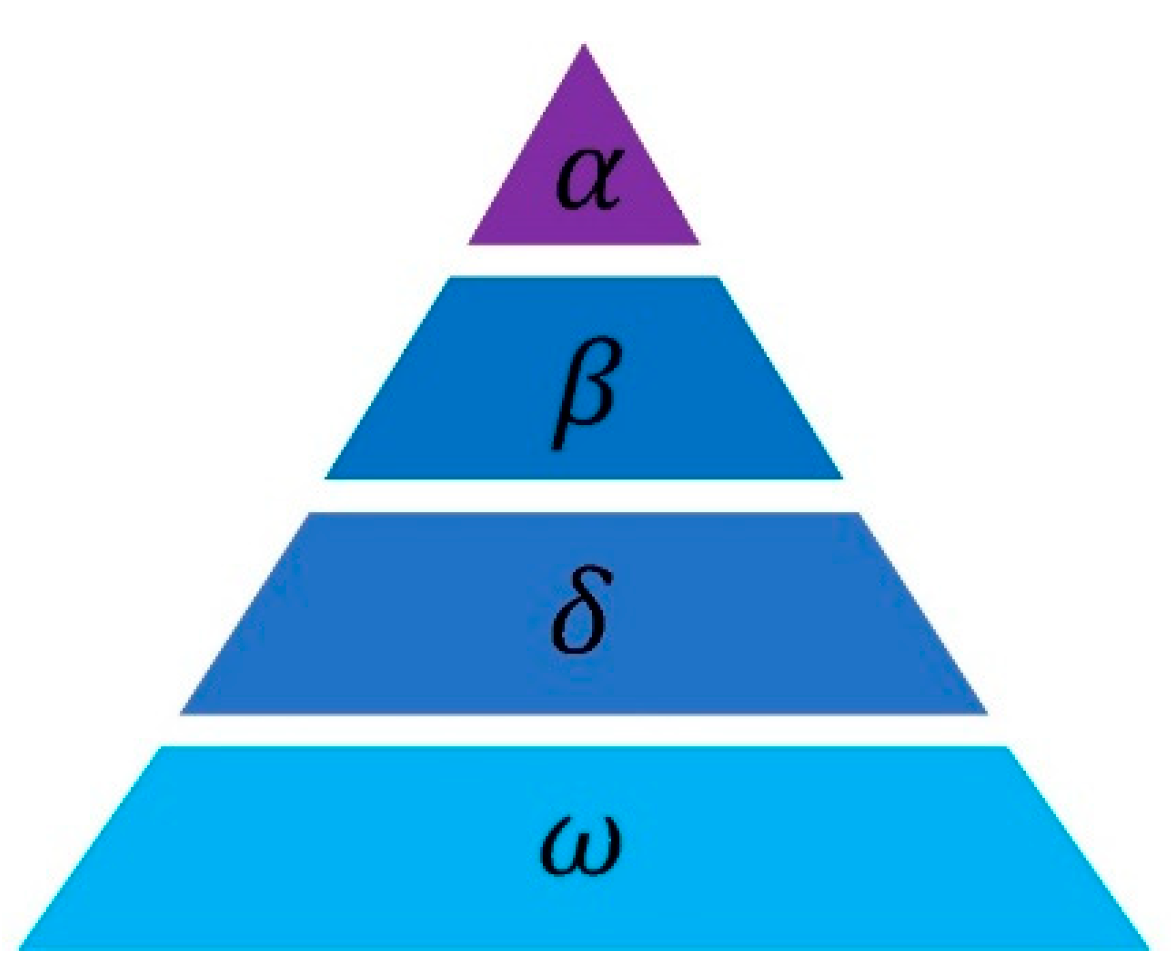
2.1. Grey Wolf Optimizer

There is a strict hierarchical distribution within the grey wolf population to balance the various responsibilities of each grey wolf. Among them, the grey wolf population is divided into four social classes for management and division of labour, as shown in Figure 1. The first level is Grey Wolf Alpha, which is the leader of the entire wolf pack and possesses the strongest leadership and management abilities; The second level is Grey Wolf Beta, which obeys alpha wolves and can dominate wolves of lower levels than itself, playing a role in coordinating feedback to the entire population; The third level is Grey Wolf δ, which obeys alpha and beta wolves and can dominate wolves of other levels; The fourth level is the Grey Wolf ω, which has the largest number and needs to obey the commands of the other three types of wolves. Although it is at the bottom of the level structure, it plays an irreplaceable role in the stable operation of the wolf pack system.
The GWO simulates the hunting behaviour of grey wolf packs. Firstly, each member of the grey wolf population scours the hunting grounds to locate and track their prey. Then, when the specific location of the hunted prey is determined, the grey wolf population will surround the prey. Due to the fact that prey will constantly change their position during the encirclement process, individuals in the corridor will also follow suit and gradually reduce the encirclement range of the prey until the prey cannot move its own position. When prey cannot move, grey wolves will attack them. This hunting process of grey wolf populations is characterized by a gradual and systematic approach towards capturing their prey.
The GWO is a population-based intelligent optimization technique that emulates the social stratification and comprehensive hunting behaviour of grey wolf populations found in the natural world. Throughout the hunting process, grey wolves initiate a search for their prey, persistently narrowing the distance separating them from their prey. To quantitatively analyze and mathematically encapsulate the dynamics of grey wolves encircling their prey developed the following mathematical model for encirclement:
D = | C · X p t X ( t ) |
X t + 1 = X p t A × D
where t represents the current number of iterations of the algorithm; D represents the distance between an individual grey wolf and its prey; X p t represents the position vector of the prey at time t ; X t + 1 represents the position vector of the grey wolf individual after updating its position; and A and C are positional parameter vectors. The position parameter vectors A and C are expressed as follows:
A = 2 · a · r 1 a
C = 2 · r 2
a = 2 ( 1 t M a x )
where A is a parameter that decreases linearly with increasing iteration times; M a x is the maximum number of iterations for the algorithm; r 1 and r 2 are random vectors distributed within the range of 0 to 1; and a is used to balance the exploration and development of the algorithm.
Grey wolves work together to encircle their prey. The hunt is usually guided by the α . If α deviates from the optimal position compared to other wolves, β and δ can also command the hunt regularly. Since the location of the prey (the optimal location) cannot be determined in advance during the search process, it is possible that the optimal location will appear next to β and δ in addition to α . The GWO ensures the continuous refinement of the top three optimal solutions and mandates that all other search agents update their positions in each iteration based on the newly determined optimal search coordinates.
D α = | C 1 · X α t X | ,   X 1 = X α t A 1 × D α
D β = | C 2 · X β t X | ,   X 2 = X β t A 2 × D β
D δ = | C 3 · X δ t X | ,   X 3 = X δ t A 3 × D δ
X t + 1 = X 1 + X 2 + X 3 3
where D α , D β , and D δ represent the distances between the α , β , and δ and their prey, respectively; X α t , X β t , and X δ t represent the positions of α , β , and δ at time t , respectively; X 1 , X 2 , and X 3 represent the position vectors of α , β , and δ after interfering with prey, respectively; and A 1 , A 2 , and A 3 represent random vectors that affect the update position of α , β , and δ .
When the grey wolves have successfully encircled their prey and the prey cannot escape, they will attack the prey. The behavioural decision-making of grey wolves during the encirclement and attack phases is governed by parameter A , which in turn determines the variation in parameter a . When the number of iterations is between 0 and M a x / 2 , the GWO algorithm executes the stage of grey wolf search and encirclement of prey. Parameter A will cause the grey wolf to abandon its current prey and search for better prey in the entire search space. When the number of iterations is between M a x / 2 and M a x , | A | < 1 , the GWO algorithm is in the stage of developing and attacking prey for grey wolves. The parameter vector C is the random position vector of the prey, reflecting the random weight of the influence of the grey wolf’s position on the current prey. The parameter vector C is a randomly distributed vector in the interval [ 0 , 2 ] . The larger the value of C , the greater the emphasis on the prey being influenced by the position of the grey wolf. When | C | 1 , it indicates that the prey is in the stage of escaping from the encirclement of grey wolves. When | C | < 1 , it indicates that the prey is being surrounded by grey wolves and is gradually losing their ability to escape.

2.2. Gaussian Mutation

The Gaussian distribution, known for its central role in statistical analysis, can be effectively utilized for mutation operations within metaheuristic algorithms. The probability density expression of Gaussian distribution is as follows:
G x = 1 2 π σ exp ( ( x μ ) 2 2 σ 2 )
where μ is the expectation and σ 2 is the variance. When μ = 0 and σ 2 = 1 , it is a standard normal distribution. The specific operational formula for Gaussian mutation is as follows:
P i G = P i ( 1 + G a u s s ( 0 , σ 2 ) )
where P i G represents the position after Gaussian mutation operation; P i is the position before the mutation operation; and G a u s s ( 0 , σ 2 ) is the Gaussian mutation operator that generates a random number that follows a standard normal distribution. Gaussian mutation is equivalent to conducting a comprehensive search on the current individual, with the extent of the search being modulated by the Gaussian distribution. When the expected value of μ = 0 , according to the Gaussian distribution law, it is highly likely that the random number generated by G x is a number near 0. At this time, individuals conduct small-scale local searches. Random numbers also have a small probability of falling around −2 or 2. In this case, individuals conduct large-scale local searches, and these regions may be potential areas for the global optimal value.

2.3. Cauchy Mutation

The Cauchy distribution can also be used for mutation operations in optimization algorithms. The probability density expression of Cauchy distribution is as follows:
C x ; x 0 , ρ = 1 π ρ [ 1 + ( x x 0 ρ ) 2 ]
where x 0 is the peak position parameter and ρ is the width parameter at the peak. When x 0 = 0 and ρ = 1 , it is called the standard Cauchy distribution. The formula for Cauchy mutation operation is as follows:
P i C = P i ( 1 + C a u c h y ( 0 , ρ ) )
where P i C is the position after Cauchy mutation operation; P i is the position before the mutation operation; and C a u c h y ( 0 , ρ ) is the Cauchy mutation operator, which functions to generate a random number that follows a standard normal distribution. The standard Cauchy distribution features a lower peak and a more extensive tail compared to the standard normal distribution. This characteristic endows Gaussian mutation with a pronounced local search capability, yet it diminishes its effectiveness in global exploration and its ability to break free from local optima. Conversely, the broader distribution range of the Cauchy mutation confers superior global search capabilities and facilitates a more straightforward escape from local optimal value.

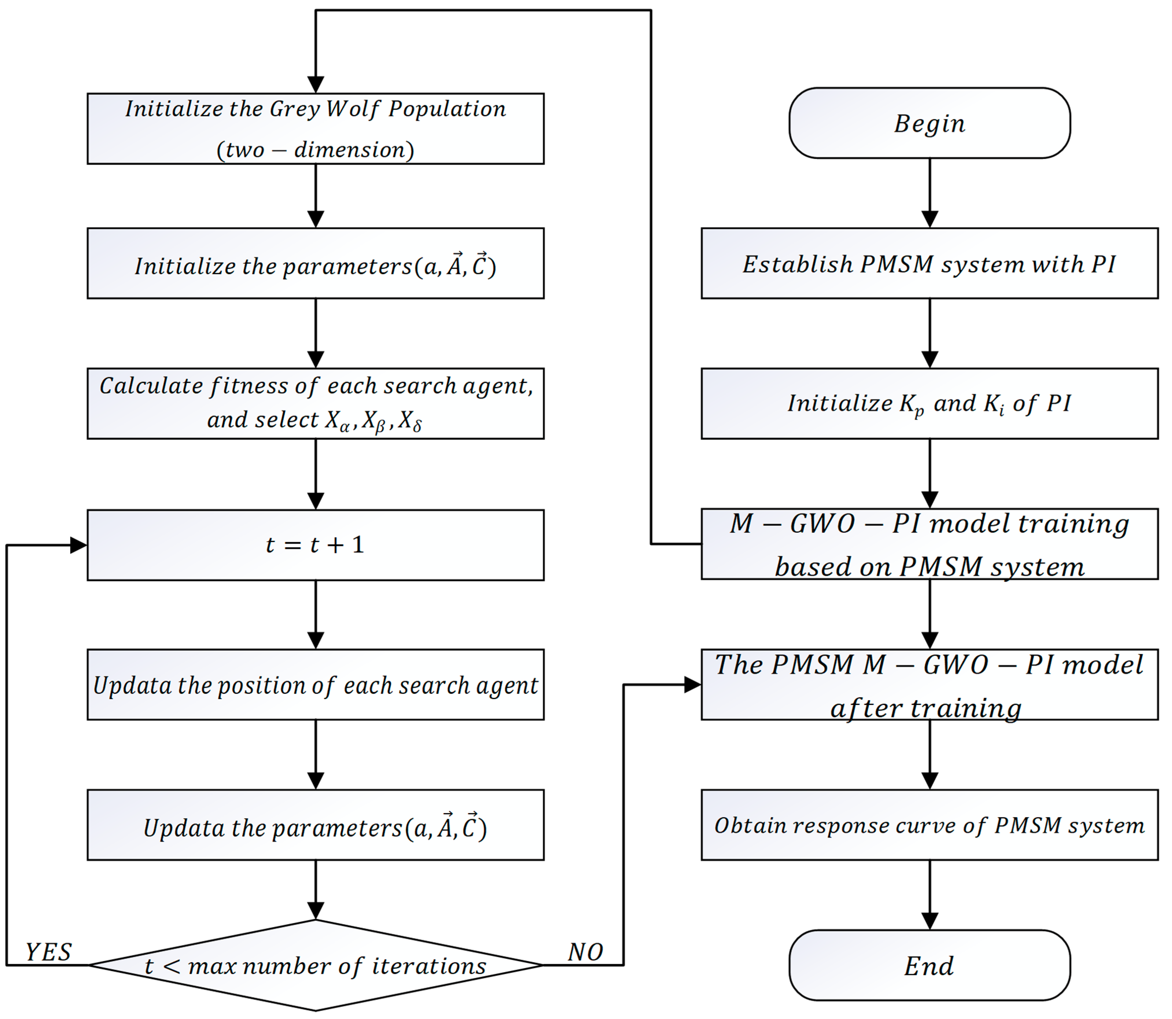
3. Modified Grey Wolf Optimizer

In GWO, ω are moved towards the α , β , and δ of the three leading wolves, which often leads to poor exploration and premature convergence. To address these limitations, we introduce an enhanced version of the Grey Wolf Optimizer, termed the Modified Grey Wolf Optimizer (M-GWO). The M-GWO algorithm has been enriched by the different behaviours of α wolves—alpha wolves typically isolate themselves from other wolves through specific location updates, exploring their territory and finding prey—and introducing mutation operators for the ω wolf to enrich its search space.
In the M-GWO, the search space is significantly expanded through the incorporation of sine and cosine functions specifically for the α wolf. The use of sine and cosine functions greatly optimizes the search space of alpha wolves. Due to its best fitness, this scheme can enable it to search for the optimal solution faster. The specific location update formula is as follows:
D α B e s t = C 1 × X α × sin r 3 X     ,   r 4 < 0.5
D α B e s t = C 1 × X α × cos r 3 X     ,   r 4 0.5
X b e s t = D α A 1 × D α B e s t
where r 3 is a random number from 0 to 2. In the M-GWO search strategy, X b e s t plays the role of the alpha wolves with the best fitness. An alpha wolf can better explore its territory, thereby improving the exploration ability of the M-GWO algorithm. The r 4 helps the alpha wolf in the M-GWO exhibit random behaviour, achieving a balance between exploration and development.
Gaussian mutation functions as a localized search mechanism for grey wolves, with the scope of this search being regulated by the Gaussian distribution. Similarly to Gaussian mutation, Cauchy mutation operation can enrich the diversity of the population, expanding the search range of individual ω wolves by introducing Gaussian mutation and Cauchy mutation. Gaussian mutation and Cauchy mutation make it easier for the M-GWO to escape local optimal value and find better solutions to avoid premature convergence. The specific formula for updating the position of individual ω wolves is
X m t = ( X 1 + X 2 + X 3 3 ) ( 1 + γ C a u c h y 0 , 1 + ( 1 γ ) G a u s s ( 0 , 1 ) )
where X m t is the position of the mutated individual of the ω wolf; C a u c h y 0 , 1 and G a u s s ( 0 , 1 ) are the standard Gauss mutation and the standard Cauchy mutation, respectively; and γ = 1 ( t / M a x ) 2 is the coefficient of mutation control, which is adaptively adjusted with the number of iterations to coordinate the local development and global exploration capabilities of the algorithm. When the value of γ is large in the early stage of iteration, the algorithm has better global exploration ability under the dominance of the Gauss mutation operator. As the iteration progresses, the local search ability of the algorithm is strengthened under the dominance of the Cauchy mutation operator. Table 1 shows the pseudo code of the M-GWO. The pseudo code can clearly demonstrate the process of algorithms, while the Cauchy mutation operator provides larger perturbations in the local search to help escape local optimal value. The introduction of Gaussian distribution further balances local and global search capabilities. The randomness of the Gaussian distribution helps maintain diversity in the global search. In conclusion, the utilization of a hybrid form of Gaussian and Cauchy distributions in the M-GWO enhances global search capabilities, increases population diversity, and improves the balance between local and global search abilities.
Compared to GWO, the M-GWO features a more sophisticated position update mechanism to address more complex problems. However, the M-GWO incorporates parameters such as the Cauchy mutation operator and the Gaussian mutation operator, which increase the algorithm’s complexity and parameter count. For example, the selection of mutation operator values and the choice of random numbers both increase computational complexity. Both the introduction of mutation operators and the improvement of the alpha wolf position update strategy introduce different variables. However, algorithms such as GWO, WOA, and DBO do not introduce too many variables, so there will not be excessive time and memory-space costs in the optimization process. As a result, the M-GWO requires more computational time compared to algorithms with fewer parameters. The pseudo-code of M-GWO is shown in Algorithm 1.
Algorithm 1 The pseudo code of M-GWO—Modified Based Grey Wolf Optimizer
1 : Initialize   the   grey   wolf   population   X i ( i = 1 , 2 ,   ,   n )
 2:  Calculate the fitness of each search agent
3 : X α is the best search agent
4 : X β is the second search agent
5 : X δ is the third search agent
 6: While   ( t < M a x number of iterations)
 7:   For each search agent
 8: If   r 4 < 0.5
9 : Update   the   position   of   α by Equation (14)
 10:    else
11 :     Update   the   position   of   α by Equation (15)
 12:    end If
13 :     Update   the   position   of   β by Equation (7)
14 :     Update   the   position   of   δ by Equation (8)
15 :     Update   the   position   of   ω by Equation (17)
 16:    end For
 17:     Update   a ,   A   and   C
 18:     Update   t = t + 1
 19:    end While
 20:     return   X α

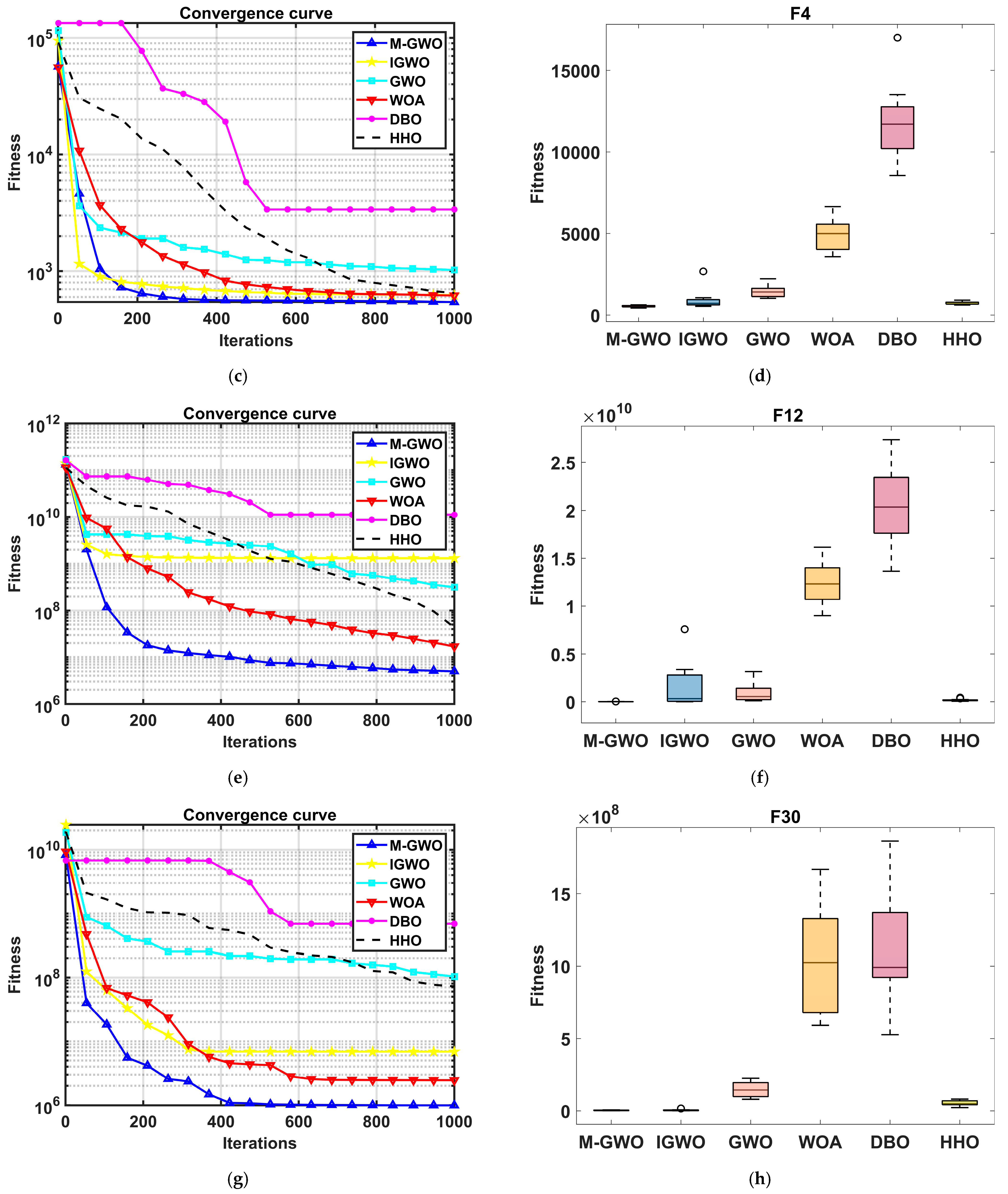
4. Experimental Evaluation and Results

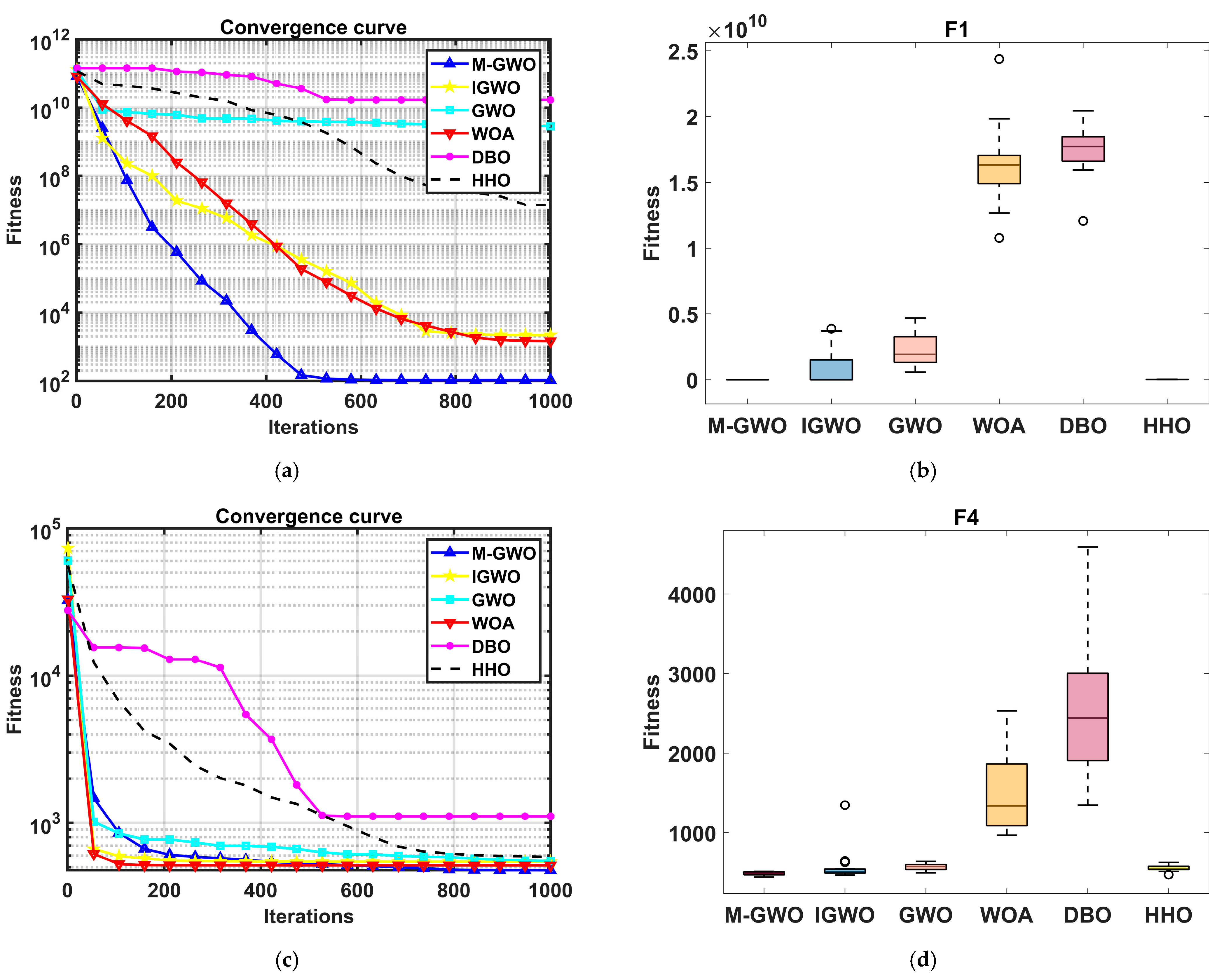
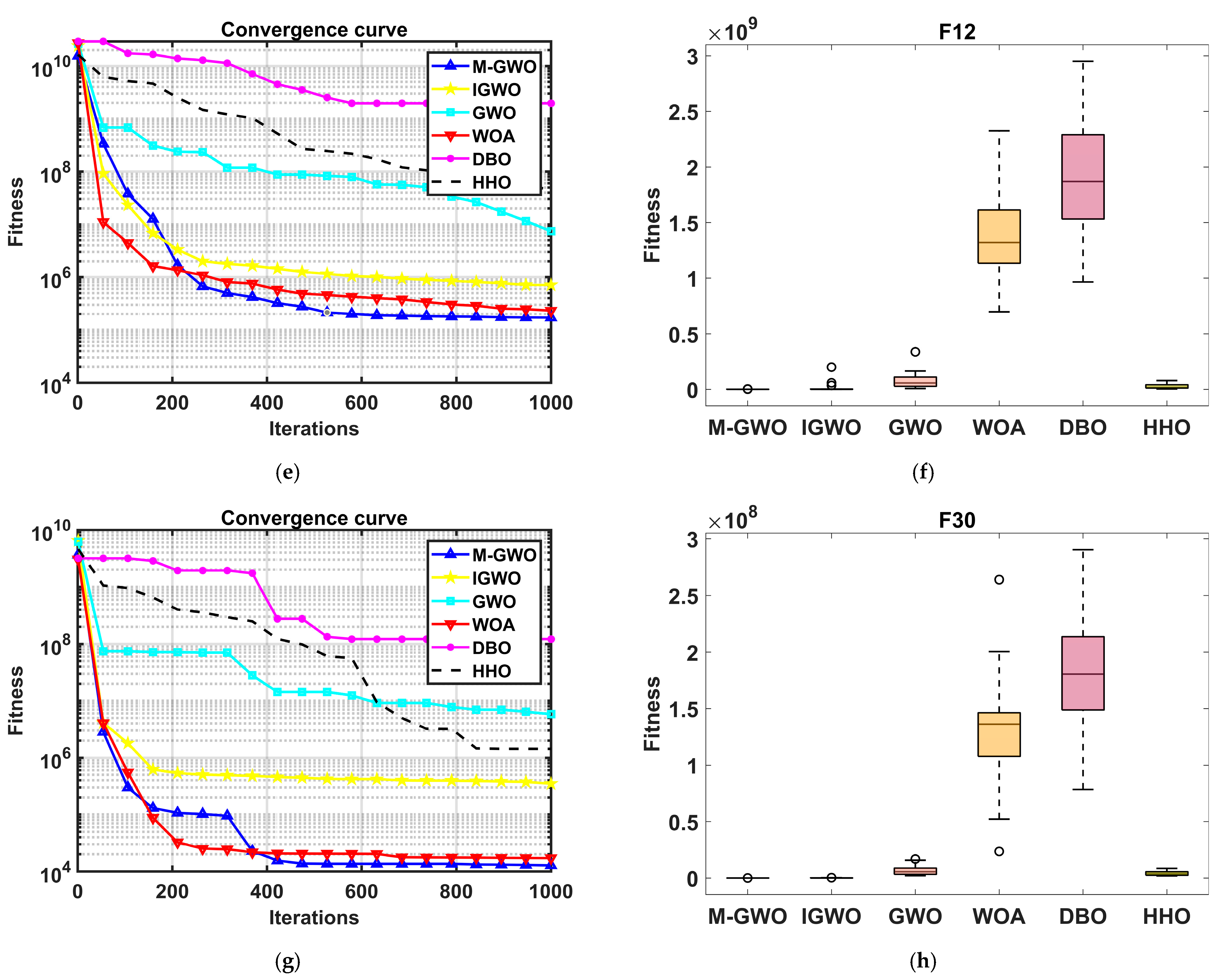
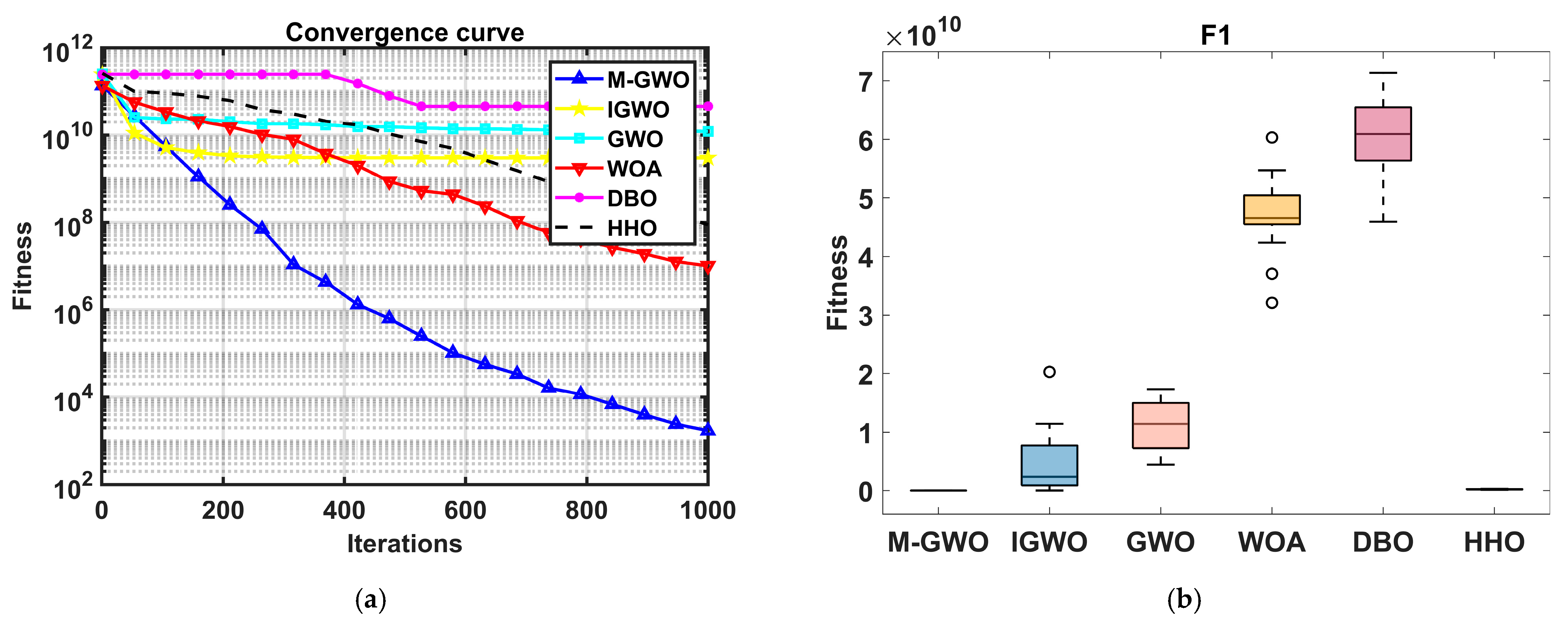
4.1. The Test Results of Benchmark Function

In this section, the performance of M-GWO was evaluated on the CEC2017 benchmark function. All testing scenarios should be conducted in the same environment to address the different results caused by the randomness of metaheuristic algorithms. All algorithms are implemented on MATLAB 2023b which is a simulation software published by MathWorks in Natick, MA, USA. The experiment was performed on an Intel Core i7-12700 CPU (2.70 GHz) with 16 GB of main memory in Lenovo laptop (Beijing, China). The CEC2017 benchmark function set includes 29 optimization problems, including unimodal functions (F1, F3), multimodal functions (F4–F10), hybrid functions (F11–F20), and composition functions (F21–F30). The specific benchmark function expression is in Appendix A. Unimodal functions, multimodal functions, hybrid functions, and composite functions can all evaluate the development and exploration capabilities of algorithms from different aspects. The CEC 2017 benchmark function used in the experiment includes different types of functions with dimensions of 30 and 50, respectively. Each algorithm undergoes 30 independent experiments separately to ensure the fairness of the experimental results. The maximum number of iterations ( M a x ) for the algorithm in the experiment is set to 1000. We evaluated the performance of the algorithm by comparing the average error, standard deviation, and minimum value of the global best solution obtained after 30 runs.
The M-GWO is compared with other cash-element heuristic algorithms. The test results of each benchmark function provide their convergence behaviour in different dimensions. In addition, the performance of each algorithm was evaluated by comparing the minimum, average, and standard deviation of the global best solution obtained after 30 runs. The statistical analysis of minimum, mean, and standard deviation can effectively demonstrate the overall effectiveness of the compared algorithms. All the parameters of the algorithms used for comparison in this article are shown in Table 1.
Table A1 shows the optimized numerical results of different algorithms on the unimodal function in the CEC2017 benchmark function. The experimental results demonstrate that the M-GWO has better performance in solving the problem of unimodal functions, therefore the M-GWO has better development capabilities. Table A2 shows the optimized numerical results of different algorithms on the multimodal function in the CEC2017 benchmark function. The experimental results demonstrate that the M-GWO has better development capabilities compared to other algorithms. Table A3 and Table A4 show the optimized numerical results of different algorithms on the mixed and composite functions in the CEC2017 benchmark function, respectively. The experimental results demonstrate that the M-GWO has a better ability to balance development and exploration.
The main reason for obtaining the experimental effect is based on the improved Grey Wolf Optimization algorithm combined with different update strategies. Firstly, the position update for alpha wolves incorporates the sine and cosine function update method. Given their superior fitness, this enhanced updated scheme allows α wolves to more effectively explore the vicinity of individuals. Secondly, Gaussian mutation and Cauchy mutation were used in the position update formula for the ω wolf. The introduction of these mutation operators bolsters the developmental capabilities of individuals, and individual mutation facilitates the escape from local optimal value.
The statistical values in Table A1, Table A2, Table A3 and Table A4 indicate that the M-GWO has better optimization capabilities compared to other algorithms. The M-GWO utilizes different location update strategies to effectively enhance optimization capability. Firstly, the position update for alpha wolves adopts the sine cosine function update method. Due to the best fitness of alpha wolves, the improved update scheme can enable them to better explore the nearby locations of individuals. Then, Gaussian mutation and Cauchy mutation were used in the position update formula for the ω wolf. The use of mutation operators can improve individual development ability, and individual mutation can break away from local optimal value.
Table A5 shows the average time required for different algorithms to perform a single optimization on CEC2017. Table A5 shows the average time required for different algorithms to perform a single optimization on CEC2017. The statistical results show that due to the increased complexity of the M-GWO, the time required for optimization of the M-GWO is not the shortest. However, the performance improvement of the M-GWO is sufficient to compensate for the shortcomings in time consumption.
Figure 2 shows the convergence curves and box plots obtained by testing different algorithms on benchmark functions F1, F4, F12, and F30 in 30 dimensions. The convergence curve shows that the M-GWO has better convergence accuracy compared to other algorithms in 30 dimensions. The box plot shows that the M-GWO has better stability compared to other algorithms under multiple independent runs in 30 dimensions. Figure 3 shows the convergence curves and box plots obtained by testing different algorithms on benchmark functions F1, F4, F12, and F30 in 50 dimensions. The convergence curve shows that the M-GWO has a faster convergence speed and better convergence accuracy compared to other algorithms in 50 dimensions. The box plot shows that the M-GWO has a smaller average compared to other algorithms under multiple independent runs in 50 dimensions. The convergence curves and box plots at different dimensions demonstrate the superior performance of the M-GWO.

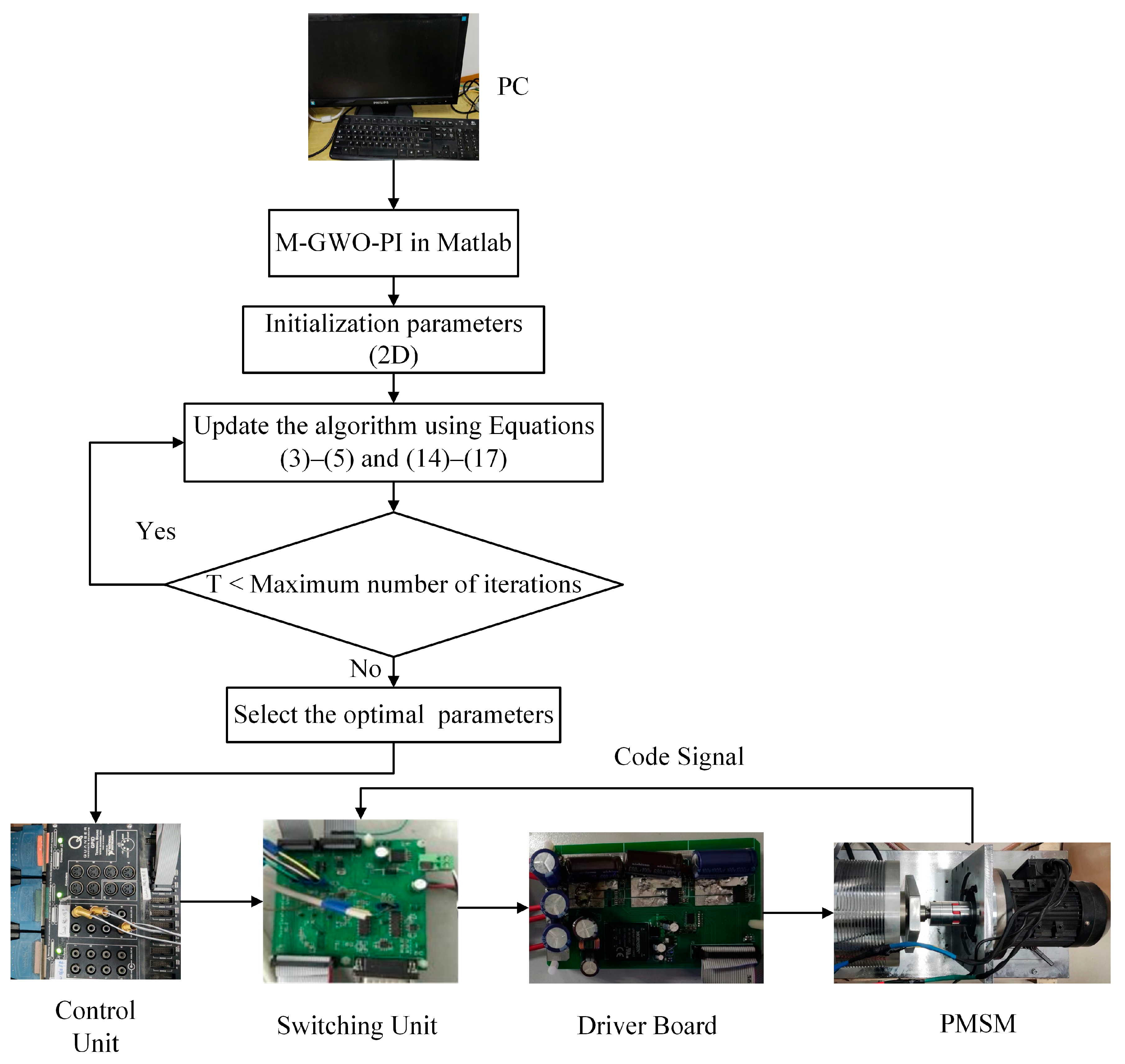
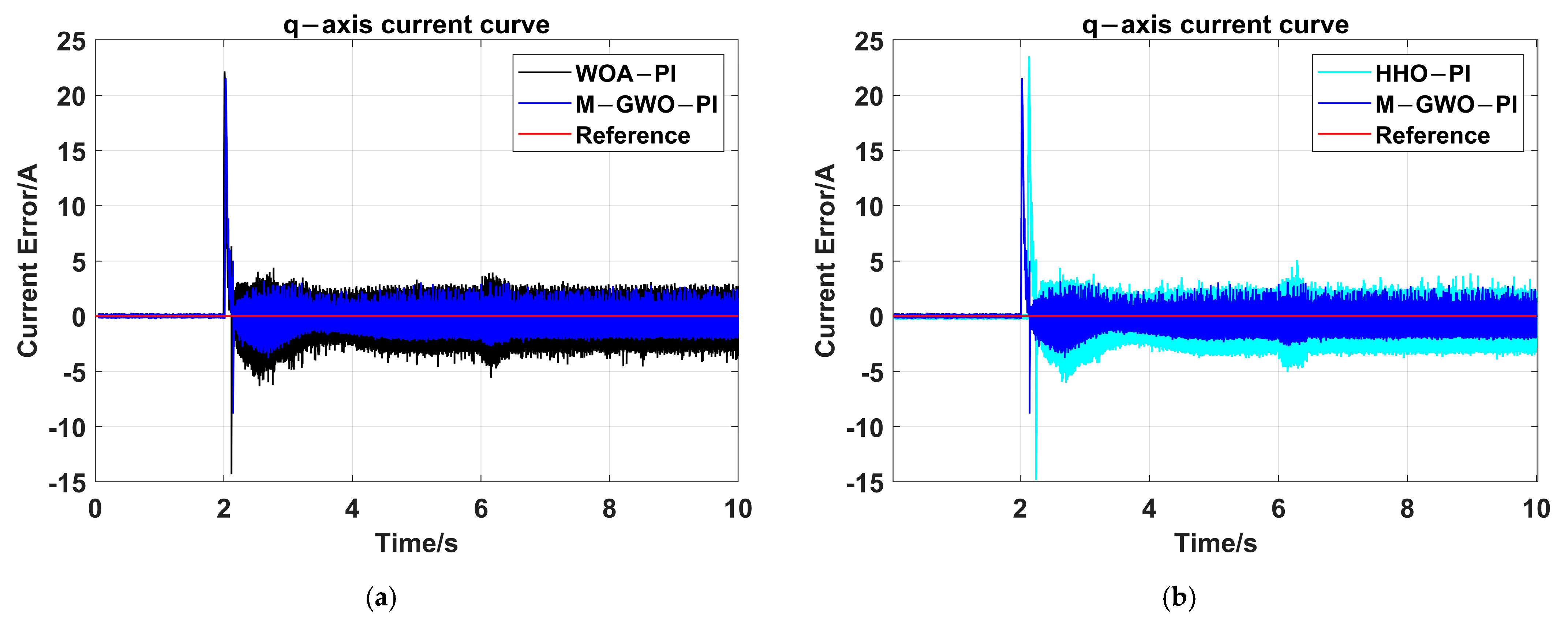
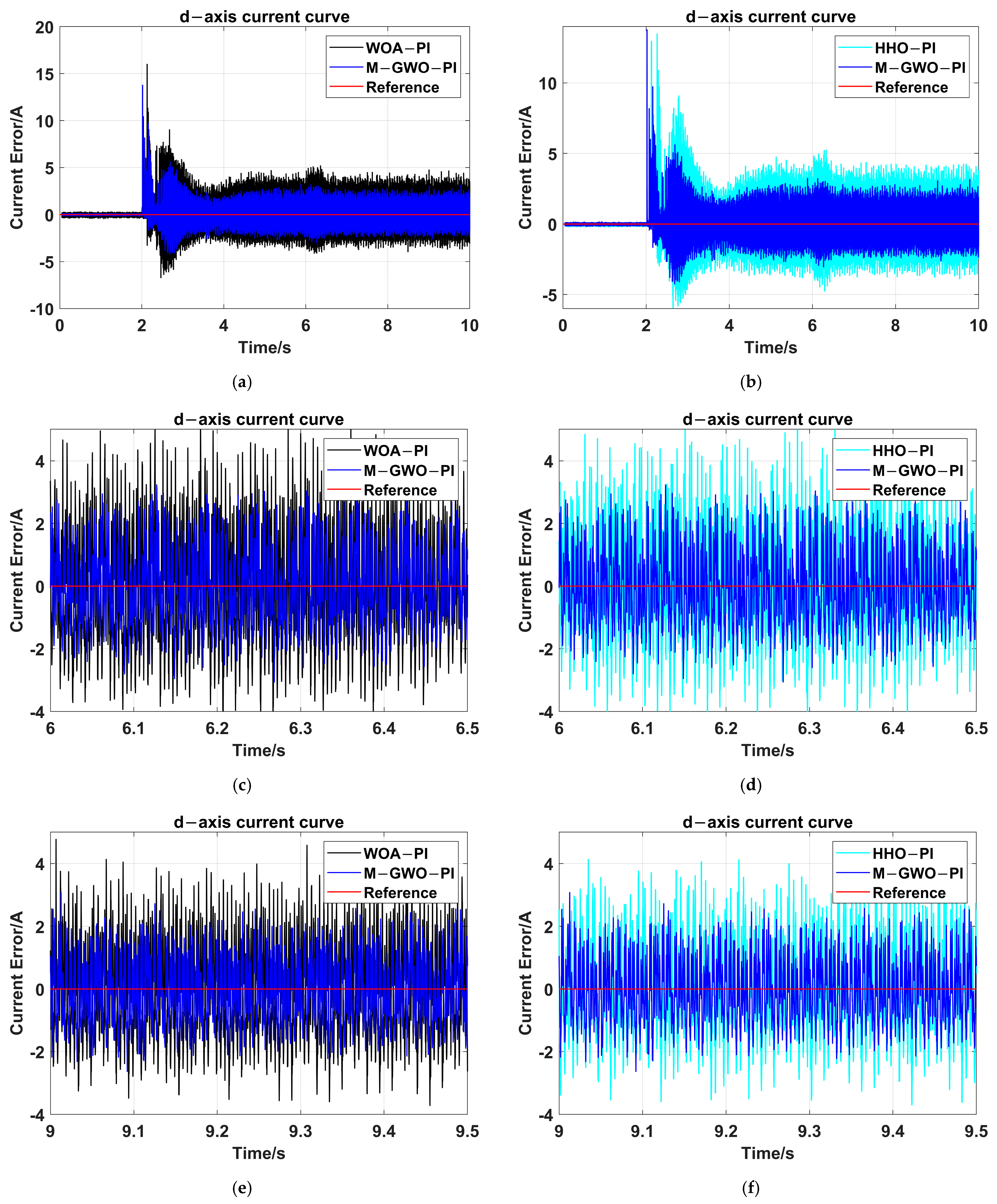
4.2. Application of M-GWO to PI Controller Parameters

The requirement of high-precision control of motors in modern industrial conditions is increasing. A permanent magnet synchronous motor (PMSM) is now widely used in various working conditions. While controlling the speed in the PMSM, the system is actually controlling the current. The current loop is the basis of the speed loop design, so that the output current can track the set current well for the system. For the PMSM system, the voltage equation of the d -axis and the q -axis is presented as follows:
U d = r · I d + d L d I d d t ω e L q I q
U q = r · I q + d L q I q d t + ω e L d I d + ω e ψ f
where L d and L q are the inductance of the d -axis and q -axis respectively; ω e is the speed; and ψ f is the permanent magnet flux link. The motor torque is directly related to I q and I d . The expression of torque as follows:
T e = 3 2 p n I q [ I d L d L q + ψ f ]
For motor control, the current loop is the most internal system of the motor. The tracking accuracy of the current loop is very important, and is related to the overall performance of the motor. The smaller the current-tracking error fluctuation value of the q-axis and d-axis, the better. At present, the parameters of the PI controller added to the current loop are usually obtained through the empirical method. The empirical method can only meet the general conditions and cannot make the system have enough control accuracy. Therefore, it is important to select the appropriate PI controller parameters in the current loop. Figure 4 shows the parameter optimization process of the M-GWO for the current loop PI controller of the PMSM system. Figure 5 shows the actual parameter optimization control system. The control unit is a 32-bit floating-point DSP processor that contains TMS320F28335 and is used to implement three-phase PWM inverter processing. A STC15W10X single-chip microcomputer plays an important role as the switching unit. The manufacturer of this device is Hardman Technology in Jiande, China. The signal from the controller is transmitted to the switching board and then to the driving board. The driving board transmits the electrical signal to the PMSM system for driving. The current situation of the PMSM system is transmitted to the converter board through the encoder adapter, and then to MATLAB for data preservation.
In the PI controller optimization, actual parameter values of the PMSM are selected. The PMSM parameters involved are shown in Table 2. To demonstrate the effectiveness of the method, it was compared with other excellent intelligent algorithms. Table 3 shows the parameters of the PI controller after system tuning using the WOA-PI, HHO-PI, and M-GWO-PI method.
A small load disturbance is given to the PMSM at six seconds. The q -axis current-tracking error between the M-GWO-PI method and WOA-PI method, and the M-GWO-PI method and HHO-PI method are compared in Figure 6. During the start-up phase, the peak current of the M-GWO-PI is lower than that of WOA-PI and HHO-PI. The startup speed of HHO-PI is significantly slower than that of the M-GWO-PI. When the reverse current occurs during the motor start-up phase, the current of the M-GWO-PI is less than 10 A. The reverse current of WOA-PI and HHO-PI reaches nearly 15 A, which is not conducive to the service life of the motor. Figure 6c,d shows that when subjected to disturbance, the method of the M-GWO-PI can exhibit smaller current fluctuations compared to other methods. Figure 6e,f shows that at around 9 s, there is a click on the motor to reach the stable stage of operation. The q-axis current of the M-GWO-PI in the stable stage is about −2~1 A, while the q-axis currents of WOA-PI and HHO-PI are both around −3~2 A.
The comparison of the d-axis current-tracking error between the M-GWO-PI method and WOA-PI method, and M-GWO-PI method and HHO-PI method are shown in Figure 7. During the start-up phase, the current response speed of M-GWO-PI is faster than that of WOA-PI and HHO-PI. Figure 7c,d shows that when subjected to disturbance, the method of the M-GWO-PI can exhibit smaller current fluctuations compared to other methods. The d-axis current fluctuations of WOA-PI and HHO-PI are greater, with peak fluctuations reaching 4 A. Figure 7e,f shows that at around 9 s, there is a click on the motor to reach the stable stage of operation. The q-axis current of the M-GWO-PI in the stable stage is about −2~2 A, while the d-axis currents of WOA-PI and HHO-PI are both around −2~3 A.

5. Conclusions

To address the challenges of inadequate exploration, reduced diversity, and the imbalance between exploration and exploitation inherent in the Grey Wolf Optimizer (GWO), this paper introduces an enhanced version of the algorithm, known as the Modified Grey Wolf Optimizer (M-GWO). The M-GWO incorporates sine and cosine search strategies, along with Gaussian and Cauchy mutation operators. This enhanced strategy empowers the algorithm to augment both the search capability and the diversity within the population. The performance of the M-GWO was rigorously assessed and statistically analyzed through the execution of the CEC 2017 benchmark functions. In the 30 dimensions, except for F26, the M-GWO has stronger performance and better average fitness values in 30 independent solutions. In 50 dimensions, the M-GWO can find better fitness values in all test functions. The experimental results demonstrate that the M-GWO algorithm has better performance compared to other advanced metaheuristic algorithms. In addition, through testing of the motor current, the control effect of the M-GWO-PI on the motor resulted in a stable q-axis current of around −2~1 A, which is superior to WOA-PI and HHO-PI. The control effect of the M-GWO-PI on the motor results in smaller fluctuations in the d-axis current of the motor, with a stable value of around −2~2 A. The experimental results of PI controller parameter optimizations prove that the designed M-GWO has a good application prospect in engineering problems.

Author Contributions

Conceptualization, L.S. and S.W.; methodology, L.S. and S.W.; software, S.W.; validation, S.W. and Z.L.; formal analysis, S.W. and Z.L.; data curation, S.W.; writing—original draft preparation, L.S. and S.W.; writing—review and editing, L.S. and S.W.; funding acquisition, L.S. All authors have read and agreed to the published version of the manuscript.

Funding

This research was funded by the Natural Science Foundation of Xinjiang Uygur Autonomous Region Prefecture under Grant 2022D01F35.

Institutional Review Board Statement

Not applicable.

Informed Consent Statement

Not applicable.

Data Availability Statement

Due to technical reasons, no public link has been established. If you need any data, please contact the second author via email.

Acknowledgments

Thanks again to all authors for their contributions in this article, including algorithm selection and simulation.

Conflicts of Interest

The authors declare no conflicts of interest.

Appendix A

The expression for basic functions is as follows:
(1)
Bent Cigar Function
f 1 x = x 1 2 + 10 6 i = 2 D x i 2
(2)
Sum of Different Power Function
f 2 x = i = 1 D | x i | i + 1
(3)
Zakharov Function
f 3 x = i = 1 D x i 2 + ( i = 1 D 0.5 x i 2 ) 2 + ( i = 1 D 0.5 x i 2 ) 4
(4)
Rosenbrock’s Function
f 4 x = i = 1 D 1 ( 100 x i x i + 1 2 + ( x i 1 ) 2 )
(5)
Rastrigin’s Function
f 5 x = i = 1 D ( x i 2 10 cos 2 π x i + 10 )
(6)
Expanded Schaffer’s F6 Function
f 6 x = g x 1 , x 2 + + g x D 1 , x D + g x D , x 1
where g x , y = 0.5 + ( s i n 2 x 2 + y 2 0.5 ) ( 1 + 0.001 ( x 2 + y 2 ) ) 2 .
(7)
Lunacek bi-Rastrgin Function
f 7 x = m i n ( i = 1 D x ^ i μ 0 2 , d D + s i = 1 D x ^ i μ 1 2 + 10 ( D i = 1 D c o s ( 2 π z ^ i ) ) )
where μ 0 = 2.5 , μ 1 = μ 0 2 d s , s = 1 1 2 D + 20 8.2 , d = 1
y = 10 ( x ο ) 100 , x ^ i = 2 s i g n x i y i + μ 0 , for i = 1 , 2 , , D , z = Λ 100 ( x ^ μ 0 )
(8)
Non-continuous Rotated Rastrigin’s Function
f 8 x = i = 1 D ( z i 2 10 cos 2 π z i + 10 )
where x ^ = M 1 5.12 ( x ο ) 100
y i = x ^ i   i f | x ^ i | 0.5 r o u n d 2 x ^ i 2   i f | x ^ i | 0.5 , for i = 1 , 2 , , D , z = M 1 Λ 10 M 2 T a s y 0.2 ( T a s z 0.2 ( y ) )
(9)
Levy Function
f 9 x = s i n 2 π w 1 + i = 1 D 1 ( w 1 1 ) 2 1 + 10 s i n 2 π w 1 + 1 + ( w D 1 ) 2 1 + s i n 2 2 π w D
where w i = 1 + x i 1 4 , i = 1 , , D .
(10)
Modified Schwefel’s Function
f 10 x = 418.9829 × D i = 1 D g ( z i )
where z i = 4.209687462275036 × 10²
and, g z i = z i sin z i 0.5   i f   | z i | 500 500 m o d z i , 500 sin 500 m o d z i , 500 z i 500 2 10000 D   i f   z i > 500 m o d z i ,   500 500 sin m o d z i , 500 500 z i + 500 2 10000 D   i f   z i < 500
(11)
High Conditioned Elliptic Function
f 11 x = i = 1 D ( 10 6 ) i 1 D 1 x i 2
(12)
Discuss Function
f 12 x = 10 6 x 1 2 + i = 2 D x i 2
(13)
Ackley’s Function
f 13 x = 20 exp 0.2 1 D i = 1 D x i 2 exp 1 D i = 1 D cos 2 π x i + 20 + e
(14)
Weierstrass Function
f 14 x = i = 1 D ( k = 0 k m a x [ a k c o s ( 2 π b k ( x i + 0.5 ) ) ] ) D k = 0 k m a x [ a k c o s ( 2 π b k · 0.5 ) ]
where a = 0.5 , b = 3 and k m a x = 20 .
(15)
Griewank’s Function
f 15 x = i = 1 D x i 2 4000 i = 1 D cos x i i + 1
(16)
Katsuura Function
f 16 x = 10 D 2 i = 1 D ( 1 + i j = 1 32 | 2 j x i r o u n d ( 2 j x i ) | 2 ) 10 D 1.2 10 D 2
(17)
HappyCat Function
f 17 x = | i = 1 D x i 2 D | 0.25 + 0.25 i = 1 D x i 2 + i = 1 D x i D + 0.5
(18)
HGBat Function
f 18 x = | i = 1 D x i 2 2 ( i = 1 D x i ) 2 | 0.5 + 0.5 i = 1 D x i 2 + i = 1 D x i D + 0.5
(19)
Expanded Griewank’s plus Rosenbrock’s Function
f 19 x = f 7 f 4 x 1 , x 2 + + f 7 f 4 x D 1 , x D + f 7 ( f 4 ( x D , x 1 ) )
(20)
Schaffer’s F7 Function
f 20 x = [ 1 D 1 i = 1 D 1 s i sin 50 s i 0.2 + 1 ] 2
where s i = x i 2 + x i + 1 2
The expression or the CEC2017 benchmark function is as follows:
  • Unimodal Functions
F 1 x = f 1 M x ο 1 + F 1 , F = 100
F 2 x = f 2 M x ο 2 + F 2 , F = 200
F 3 x = f 3 M x ο 3 + F 3 , F = 300
F 4 x = f 4 M 2.048 x ο 4 100 + 1 + F 4 , F = 400
F 5 x = f 5 M x ο 1 + F 5 , F = 500
F 6 x = f 20 M 0.5 x ο 6 100 + F 6 , F = 600
F 7 x = f 7 M 600 x ο 7 100 + F 7 , F = 700
F 8 x = f 8 M 5.12 x ο 8 100 + F 8 , F = 800
F 9 x = f 9 M 5.12 x ο 9 100 + F 9 , F = 900
F 10 x = f 10 M 1000 x ο 10 100 + F 10 , F = 1000
B.
Hybrid Functions
Parameters: N is the number of basic functions; p is used to control the proportion of g i ( x ) . The expression of hybrid function is F x = i = 1 N g i ( M i z i ) + F
F 11 : N = 3 , p = [ 0.2,0.4,0.4 ]   g 1 : f 3 , g 2 : f 4 , g 3 : f 5
F 12 : N = 3 , p = [ 0.3,0.3,0.4 ]   g 1 : f 11 , g 2 : f 10 , g 3 : f 1
F 13 : N = 3 , p = [ 0.3,0.3,0.4 ]   g 1 : f 1 , g 2 : f 4 , g 3 : f 7
F 14 : N = 4 , p = [ 0.2,0.2,0.2,0.4 ]   g 1 : f 11 , g 2 : f 13 , g 3 : f 20 , g 4 : f 5
F 15 : N = 4 , p = [ 0.2,0.2,0.3,0.3 ]   g 1 : f 11 , g 2 : f 13 , g 3 : f 20 , g 4 : f 5
F 16 : N = 4 , p = [ 0.2,0.2,0.3,0.3 ]   g 1 : f 6 , g 2 : f 18 , g 3 : f 4 , g 4 : f 10
F 17 : N = 5 , p = [ 0.1,0.2,0.2,0.2,0.3 ]   g 1 : f 16 , g 2 : f 13 , g 3 : f 5 , g 4 : f 18 , g 5 : f 12
F 18 : N = 5 , p = [ 0.2,0.2,0.2,0.2,0.2 ]   g 1 : f 1 , g 2 : f 13 , g 3 : f 5 , g 4 : f 18 , g 5 : f 12
F 19 : N = 5 , p = [ 0.2,0.2,0.2,0.2,0.2 ]   g 1 : f 1 , g 2 : f 5 , g 3 : f 19 , g 4 : f 14 , g 5 : f 6
F 20 : N = 6 , p = [ 0.1,0.1,0.2,0.2,0.2,0.2 ]   g 1 : f 17 , g 2 : f 16 , g 3 : f 13 , g 4 : f 5 , g 5 : f 10 , g 6 : f 20
C.
Composite Functions
Parameters: σ i is the new optimal moving position for each function; b i a s i is the global optimal value; w i = 1 j = 1 D ( x j o i j ) 2 e x p ( j = 1 D ( x j o i j ) 2 2 D σ i 2 ) ; and ω i = w i / i = 1 n w i . The expression of composite function is F x = i = 1 N { ω i [ λ i g i x + b i a s i ] } + F
F 21 : N = 3 , σ = [ 10 , 20 , 30 ] , λ = [ 1 , 1 × 10 6 , 1 ] , b i a s i = [ 0 , 100 , 200 ]   g 1 : f 5 , g 2 : f 11 , g 3 : f 4
F 22 : N = 3 , σ = [ 10 , 20 , 30 ] , λ = [ 1 , 10 , 1 ] , b i a s i = [ 0 , 100 , 200 ]   g 1 : f 5 , g 2 : f 15 , g 3 : f 10
F 23 : N = 4 , σ = [ 10 , 20 , 30 , 40 ] , λ = [ 1 , 10 , 1 ] , b i a s i = [ 0 , 100 , 200 , 300 ]   g 1 : f 4 , g 2 : f 13 , g 3 : f 10 , g 4 : f 5
F 24 : N = 4 , σ = [ 10 , 20 , 30 , 40 ] , λ = [ 10 , 1 × 10 6 , 10 , 1 ] , b i a s i = [ 0 , 100 , 200 , 300 ]   g 1 : f 13 , g 2 : f 11 , g 3 : f 15 , g 4 : f 5
F 25 : N = 5 , σ = [ 10 , 20 , 30 , 40 , 50 ] , λ = [ 10 , 1 , 1 × 10 6 , 10 , 1 ] , b i a s i = [ 0 , 100 , 200 , 300 , 400 ]   g 1 : f 5 , g 2 : f 17 , g 3 : f 13 , g 4 : f 12 , g 5 : f 4
F 26 : N = 5 , σ = [ 10 , 20 , 30 , 40 , 50 ] , λ = [ 1 × 10 26 , 10 , 1 × 10 6 , 10 , 5 × 10 4 ] , b i a s i = [ 0 , 100 , 200 , 300 , 400 ]   g 1 : f 6 , g 2 : f 10 , g 3 : f 15 , g 4 : f 4 , g 5 : f 5
F 27 : N = 6 , σ = [ 10 , 20 , 30 , 40 , 50 , 60 ] , λ = [ 10 , 10 , 2.5 , 1 × 10 26 , 1 × 10 6 , 5 × 10 4 ] , b i a s i = [ 0 , 100 , 200 , 300 , 400 , 500 ]   g 1 : f 18 , g 2 : f 5 , g 3 : f 10 , g 4 : f 1 , g 5 : f 11 , g 6 : f 6
F 28 : N = 6 , σ = [ 10 , 20 , 30 , 40 , 50 , 60 ] , λ = [ 10 , 10 , 1 × 10 6 , 1 , 1 , 5 × 10 4 ] , b i a s i = [ 0 , 100 , 200 , 300 , 400 , 500 ]   g 1 : f 13 , g 2 : f 15 , g 3 : f 12 , g 4 : f 4 , g 5 : f 17 , g 6 : f 6
F 29 : N = 3 , σ = [ 10 , 30 , 50 ] , λ = [ 1 , 1 , 1 ] , b i a s i = [ 0 , 100 , 200 ]   g 1 : F 5 , g 2 : F 6 , g 3 : F 7
F 30 : N = 3 , σ = [ 10 , 30 , 50 ] , λ = [ 1 , 1 , 1 ] , b i a s i = [ 0 , 100 , 200 ]   g 1 : F 5 , g 2 : F 8 , g 3 : F 9

Appendix B

Below are the optimization result statistics of the M-GWO and other optimization algorithms for hybrid functions and composite functions. Table A1 shows the results of the M-GWO and competitor algorithms on unimodal functions. Table A2 shows the results of the M-GWO and competitor algorithms on multimodal functions. Table A3 shows the results of the M-GWO and competitor algorithms on hybrid functions. Table A4 shows the results of the M-GWO and competitor algorithms on composite functions.
Table A1. The results of the M-GWO and competitor algorithms on unimodal functions.
FunctionDimIndexM-GWOIGWOGWOWOADBOHHO
F130Min1.07 × 1021.18 × 1025.19 × 1092.06 × 1028.21 × 10101.29 × 108
Mean4.41 × 1039.34 × 1032.87 × 10101.12 × 10102.28 × 10112.58 × 108
SD6.16 × 1038.32 × 1032.38 × 10101.97 × 10103.15 × 10105.42 × 107
50Min2.69 × 1023.21 × 1041.51 × 1064.17 × 1092.96 × 10101.22 × 108
Mean3.67 × 1038.43 × 1054.04 × 1091.15 × 10104.21 × 10101.93 × 108
SD3.02 × 1031.01 × 1064.45 × 1095.19 × 1093.96 × 1094.61 × 107
F330Min1.99 × 1052.47 × 1053.35 × 1052.46 × 1052.28 × 1052.58 × 105
Mean2.96 × 1053.84 × 1055.02 × 1053.84 × 1054.02 × 1053.62 × 105
SD5.38 × 1037.68 × 1031.07 × 1055.39 × 1032.01 × 1057.46 × 103
50Min7.22 × 1048.23 × 1042.42 × 1051.72 × 1051.02 × 1051.01 × 105
Mean1.28 × 1051.38 × 1051.59 × 1051.36 × 1051.51 × 1051.34 × 105
SD2.21 × 1043.75 × 1045.02 × 1041.69 × 1042.85 × 1042.01 × 104
Table A2. The results of the M-GWO and competitor algorithms on multimodal functions.
FunctionDimIndexM-GWOIGWOGWOWOADBOHHO
F430Min4.04 × 1024.75 × 1025.06 × 1024.71 × 1028.21 × 1024.95 × 102
Mean4.90 × 1026.00 × 1026.72 × 1024.98 × 1021.26 × 1035.44 × 102
SD3.45 × 1012.24 × 1023.60 × 1022.80 × 1013.92 × 1022.79 × 101
50Min4.34 × 1024.59 × 1026.08 × 1024.81 × 1021.05 × 1036.36 × 102
Mean5.50 × 1021.06 × 1031.36 × 1035.63 × 1021.62 × 1037.63 × 102
SD6.97 × 1016.49 × 1023.91 × 1027.58 × 1011.16 × 1037.51 × 101
F530Min5.62 × 1025.71 × 1026.21 × 1026.29 × 1026.82 × 1026.42 × 102
Mean6.16 × 1026.26 × 1027.23 × 1027.37 × 1026.99 × 1027.59 × 102
SD4.19 × 1014.19 × 1015.62 × 1015.12 × 1014.23 × 1014.17 × 101
50Min6.32 × 1026.76 × 1027.58 × 1028.19 × 1028.22 × 1028.67 × 102
Mean7.45 × 1027.62 × 1028.49 × 1028.76 × 1021.17 × 1039.17 × 102
SD3.66 × 1014.89 × 1013.12 × 1012.87 × 1014.49 × 1012.86 × 101
F630Min6.00 × 1026.03 × 1026.16 × 1026.29 × 1026.25 × 1026.49 × 102
Mean6.10 × 1026.12 × 1026.41 × 1026.48 × 1026.36 × 1006.63 × 102
SD4.25 × 1008.45 × 1001.44 × 1011.05 × 1015.29 × 1005.67 × 100
50Min6.10 × 1026.13 × 1026.30 × 1026.47 × 1026.52 × 1026.68 × 102
Mean6.22 × 1026.31 × 1026.55 × 1026.61 × 1026.72 × 1026.78 × 102
SD5.31 × 1001.19 × 1018.97 × 1007.61 × 1008.81 × 1005.07 × 100
F730Min7.87 × 1028.17 × 1028.57 × 1029.91 × 1021.12 × 1031.13 × 103
Mean8.42 × 1028.95 × 1021.05 × 1031.21 × 1031.22 × 1031.31 × 103
SD3.45 × 1015.12 × 1011.29 × 1029.66 × 1015.02 × 1016.73 × 101
50Min8.79 × 1029.38 × 1021.16 × 1031.38 × 1031.22 × 1031.64 × 103
Mean1.04 × 1031.10 × 1031.52 × 1031.72 × 1031.66 × 1031.86 × 103
SD1.02 × 1026.98 × 1012.03 × 1021.01 × 1024.49 × 1011.03 × 102
F830Min8.55 × 1028.74 × 1028.82 × 1029.19 × 1021.01 × 1039.07 × 102
Mean9.02 × 1029.13 × 1029.57 × 1029.79 × 1021.06 × 1039.82 × 102
SD3.37 × 1012.46 × 1013.32 × 1013.28 × 1012.33 × 1013.06 × 101
50Min9.38 × 1021.04 × 1031.14 × 1039.61 × 1021.35 × 1031.15 × 103
Mean1.04 × 1031.18 × 1031.19 × 1031.05 × 1031.49 × 1031.21 × 103
SD6.40 × 1014.34 × 1012.41 × 1013.64 × 1014.31 × 1013.29 × 101
F930Min9.25 × 1021.12 × 1032.41 × 1033.03 × 1033.32 × 1035.62 × 103
Mean2.37 × 1032.56 × 1034.95 × 1035.14 × 1046.69 × 1038.34 × 103
SD9.08 × 1022.04 × 1038.26 × 1024.90 × 1024.15 × 1039.37 × 102
50Min2.71 × 1031.18 × 1044.33 × 1031.13 × 1041.08 × 1042.01 × 104
Mean9.84 × 1031.39 × 1047.62 × 1031.31 × 1042.88 × 1042.83 × 104
SD4.97 × 1034.16 × 1031.54 × 1048.26 × 1024.53 × 1033.35 × 103
F1030Min2.84 × 1033.26 × 1033.59 × 1033.82 × 1035.22 × 1034.60 × 103
Mean4.51 × 1034.86 × 1034.98 × 1035.37 × 1036.61 × 1035.99 × 103
SD7.98 × 1021.30 × 1035.10 × 1026.68 × 1024.71 × 1027.60 × 102
50Min4.93 × 1036.09 × 1036.59 × 1036.64 × 1031.05 × 1047.40 × 103
Mean6.97 × 1037.89 × 1037.96 × 1038.83 × 1031.46 × 1049.78 × 103
SD1.00 × 1031.57 × 1039.17 × 1029.02 × 1026.92 × 1021.31 × 103
Table A3. The results of the M-GWO and competitor algorithms on hybrid functions.
FunctionDimIndexM-GWOIGWOGWOWOADBOHHO
F1130Min1.14 × 1031.17 × 1031.36 × 1031.21 × 1032.15 × 1031.21 × 103
Mean1.27 × 1031.34 × 1032.15 × 1031.33 × 1032.28 × 1031.29 × 103
SD7.11 × 1018.19 × 1019.27 × 1028.20 × 1012.47 × 1025.21 × 101
50Min1.30 × 1031.26 × 1032.05 × 1031.22 × 1032.15 × 1031.41 × 103
Mean1.47 × 1031.49 × 1035.88 × 1031.36 × 1034.55 × 1031.69 × 103
SD8.20 × 1012.86 × 1021.87 × 1037.35 × 1013.52 × 1031.07 × 102
F1230Min6.79 × 1044.16 × 1041.67 × 1056.79 × 1046.18 × 1074.78 × 106
Mean4.93 × 1051.29 × 1061.07 × 1084.93 × 1053.11 × 1082.40 × 107
SD4.61 × 1051.07 × 1064.42 × 1084.61 × 1054.18 × 1071.85 × 107
50Min1.46 × 1065.32 × 1067.42 × 1063.96 × 1076.85 × 1074.71 × 107
Mean5.45 × 1061.66 × 1071.72 × 1091.43 × 1092.28 × 1081.75 × 108
SD2.88 × 1061.19 × 1072.61 × 1091.91 × 1095.29 × 1071.09 × 108
F1330Min3.07 × 1035.89 × 1031.92 × 1032.36 × 1073.32 × 1062.64 × 105
Mean2.29 × 1043.68 × 1043.83 × 1071.50 × 1078.13 × 1065.36 × 105
SD2.53 × 1042.57 × 1041.93 × 1083.68 × 1074.52 × 1061.79 × 105
50Min8.62 × 1031.44 × 1044.61 × 1048.17 × 1053.32 × 1062.31 × 106
Mean2.98 × 1047.10 × 1041.48 × 1085.15 × 1084.81 × 1065.42 × 106
SD1.76 × 1044.21 × 1041.32 × 1089.07 × 1082.29 × 1063.58 × 106
F1430Min3.53 × 1043.64 × 1036.39 × 1039.77 × 1032.45 × 1051.05 × 104
Mean2.88 × 1035.67 × 1046.95 × 1045.05 × 1051.62 × 1065.67 × 105
SD3.16 × 1046.43 × 1045.17 × 1046.20 × 1051.39 × 1068.48 × 105
50Min2.36 × 1046.32 × 1044.07 × 1042.13 × 1052.41 × 1061.39 × 105
Mean1.69 × 1053.77 × 1051.26 × 1061.33 × 1067.19 × 1062.45 × 106
SD1.09 × 1052.99 × 1052.62 × 1061.51 × 1063.96 × 1061.99 × 106
F1530Min1.95 × 1032.03 × 1032.24 × 1032.01 × 1042.07 × 1063.30 × 104
Mean1.04 × 1041.40 × 1041.46 × 1042.41 × 1067.37 × 1068.71 × 104
SD1.33 × 1041.39 × 1041.43 × 1046.36 × 1065.53 × 1064.82 × 104
50Min2.36 × 1046.32 × 1044.07 × 1042.13 × 1059.85 × 1061.39 × 105
Mean1.69 × 1053.77 × 1051.26 × 1061.33 × 1061.93 × 1072.45 × 106
SD1.09 × 1052.99 × 1052.62 × 1061.51 × 1069.96 × 1061.99 × 106
F1630Min1.76 × 1032.15 × 1032.36 × 1032.34 × 1032.58 × 1032.38 × 103
Mean2.49 × 1032.63 × 1032.86 × 1032.98 × 1033.64 × 1033.51 × 103
SD3.22 × 1023.09 × 1023.86 × 1023.71 × 1022.69 × 1024.93 × 102
50Min2.63 × 1034.28 × 1034.09 × 1041.62 × 1083.61 × 1053.21 × 103
Mean1.59 × 1043.18 × 1041.43 × 1076.98 × 1087.11 × 1052.19 × 104
SD1.11 × 1042.26 × 1041.85 × 1072.19 × 1083.42 × 1051.91 × 104
F1730Min1.81 × 1031.89 × 1032.06 × 1032.10 × 1032.21 × 1032.05 × 103
Mean2.04 × 1032.23 × 1032.42 × 1032.29 × 1032.42 × 1032.62 × 103
SD1.67 × 1021.98 × 1022.10 × 1022.57 × 1022.01 × 1022.92 × 102
50Min2.37 × 1032.39 × 1032.69 × 1032.81 × 1033.52 × 1032.73 × 103
Mean2.85 × 1033.18 × 1033.26 × 1033.61 × 1034.71 × 1033.79 × 103
SD2.77 × 1023.32 × 1023.89 × 1023.85 × 1024.13 × 1025.01 × 102
F1830Min2.12 × 1046.77 × 1049.68 × 1049.78 × 1043.28 × 1051.23 × 105
Mean3.01 × 1055.91 × 1057.13 × 1052.11 × 1061.02 × 1061.64 × 106
SD2.92 × 1054.69 × 1051.39 × 1064.81 × 1067.79 × 1052.29 × 106
50Min2.52 × 1056.13 × 1055.28 × 1051.03 × 1062.23 × 1071.12 × 106
Mean1.53 × 1062.79 × 1063.55 × 1061.21 × 1074.51 × 1074.94 × 106
SD1.31 × 1062.11 × 1062.87 × 1061.67 × 1072.36 × 1074.09 × 106
F1930Min2.29 × 1032.09 × 1031.63 × 1042.06 × 1033.32 × 1047.39 × 104
Mean9.51 × 1032.19 × 1043.16 × 1061.34 × 1046.21 × 1048.47 × 105
SD1.13 × 1043.94 × 1048.83 × 1061.36 × 1044.52 × 1047.52 × 105
50Min2.34 × 1034.51 × 1033.35 × 1043.73 × 1032.19 × 1052.25 × 105
Mean1.86 × 1043.56 × 1051.38 × 1072.53 × 1045.31 × 1051.54 × 106
SD1.64 × 1041.66 × 1062.82 × 1071.27 × 1042.08 × 1051.07 × 106
F2030Min2.13 × 1032.25 × 1032.27 × 1032.29 × 1032.52 × 1032.41 × 103
Mean2.43 × 1034.46 × 1032.67 × 1032.75 × 1032.71 × 1032.72 × 103
SD2.10 × 1021.81 × 1022.21 × 1022.40 × 1021.36 × 1022.07 × 102
50Min2.42 × 1032.56 × 1032.76 × 1033.02 × 1033.04 × 1033.03 × 103
Mean2.91 × 1033.01 × 1033.56 × 1033.57 × 1033.41 × 1033.55 × 103
SD2.83 × 1023.18 × 1024.12 × 1022.33 × 1022.37 × 1022.77 × 102
Table A4. The results of the M-GWO and competitor algorithms on composite functions.
FunctionDimIndexM-GWOIGWOGWOWOADBOHHO
F2130Min2.35 × 1032.37 × 1032.41 × 1032.41 × 1012.42 × 1032.23 × 103
Mean2.40 × 1032.43 × 1032.47 × 1032.51 × 1032.48 × 1032.57 × 103
SD2.88 × 1013.23 × 1013.81 × 1016.71 × 1012.92 × 1018.64 × 101
50Min2.47 × 1032.53 × 1032.46 × 1032.57 × 1032.71 × 1032.73 × 103
Mean2.54 × 1032.64 × 1012.57 × 1032.77 × 1032.82 × 1032.87 × 103
SD5.61 × 1016.02 × 1017.51 × 1011.08 × 1023.41 × 1017.49 × 101
F2230Min2.30 × 1032.30 × 1032.39 × 1032.30 × 1033.28 × 1032.33 × 103
Mean3.83 × 1034.40 × 1034.56 × 1035.55 × 1034.12 × 1036.76 × 103
SD2.08 × 1031.89 × 1031.84 × 1032.22 × 1032.78 × 1021.77 × 103
50Min7.53 × 1038.53 × 1037.45 × 1038.18 × 1031.03 × 1049.96 × 103
Mean9.24 × 1039.76 × 1039.81 × 1031.02 × 1041.51 × 1041.19 × 104
SD1.05 × 1038.78 × 1022.05 × 1039.64 × 1026.33 × 1021.01 × 103
F2330Min2.71 × 1032.77 × 1032.78 × 1032.78 × 1032.87 × 1033.08 × 103
Mean2.78 × 1032.86 × 1032.93 × 1032.92 × 1032.96 × 1033.21 × 103
SD4.87 × 1016.20 × 1018.75 × 1019.08 × 1012.63 × 1011.21 × 102
50Min2.94 × 1032.92 × 1032.96 × 1033.08 × 1033.32 × 1033.51 × 103
Mean3.03 × 1033.25 × 1033.31 × 1033.38 × 1033.40 × 1033.79 × 103
SD8.21 × 1011.52 × 1021.49 × 1021.62 × 1023.22 × 1011.52 × 102
F2430Min2.89 × 1032.89 × 1032.97 × 1032.94 × 1033.09 × 1033.09 × 103
Mean2.93 × 1033.03 × 1033.09 × 1033.07 × 1033.15 × 1033.42 × 103
SD6.67 × 1016.97 × 1019.56 × 1018.28 × 1012.22 × 1011.56 × 102
50Min3.06 × 1033.20 × 1033.27 × 1033.34 × 1033.46 × 1033.75 × 103
Mean3.22 × 1033.36 × 1033.56 × 1033.54 × 1033.59 × 1034.27 × 103
SD9.50 × 1011.25 × 1021.66 × 1021.10 × 1022.31 × 1012.15 × 102
F2530Min2.88 × 1032.89 × 1032.95 × 1032.88 × 1033.01 × 1032.89 × 103
Mean2.89 × 1032.91 × 1033.04 × 1032.90 × 1033.23 × 1032.93 × 103
SD1.26 × 1014.57 × 1018.55 × 1011.61 × 1011.87 × 1021.91 × 101
50Min3.00 × 1033.01 × 1033.31 × 1033.03 × 1033.22 × 1033.14 × 103
Mean3.04 × 1033.08 × 1033.83 × 1033.14 × 1033.61 × 1033.25 × 103
SD2.11 × 1013.52 × 1013.64 × 1029.22 × 1011.26 × 1028.79 × 101
F2630Min2.90 × 1033.28 × 1033.65 × 1032.80 × 1033.12 × 1033.20 × 103
Mean5.57 × 1034.84 × 1034.91 × 1035.97 × 1033.34 × 1037.30 × 103
SD1.23 × 1031.05 × 1034.81 × 1021.35 × 1031.41 × 1021.47 × 103
50Min2.92 × 1035.64 × 1033.53 × 1032.90 × 1033.15 × 1034.05 × 103
Mean5.76 × 1036.99 × 1037.46 × 1036.93 × 1035.28 × 1031.08 × 104
SD3.61 × 1037.46 × 1021.45 × 1033.72 × 1033.75 × 1031.93 × 103
F2730Min3.20 × 1033.20 × 1033.21 × 1033.22 × 1032.26 × 1033.26 × 103
Mean3.25 × 1033.29 × 1033.26 × 1033.26 × 1033.31 × 1033.53 × 103
SD2.77 × 1015.08 × 1023.18 × 1013.19 × 1014.42 × 1011.68 × 102
50Min3.34 × 1033.36 × 1033.44 × 1033.59 × 1033.46 × 1033.80 × 103
Mean3.49 × 1033.70 × 1033.65 × 1033.75 × 1033.71 × 1034.52 × 103
SD1.33 × 1022.93 × 1029.89 × 1011.02 × 1022.22 × 1024.03 × 102
F2830Min3.02 × 1033.21 × 1033.32 × 1033.20 × 1033.20 × 1033.27 × 103
Mean3.10 × 1033.29 × 1033.45 × 1033.24 × 1033.31 × 1033.33 × 103
SD2.77 × 1011.50 × 1027.63 × 1012.79 × 1013.36 × 1024.71 × 101
50Min3.30 × 1033.33 × 1033.73 × 1033.27 × 1033.44 × 1033.53 × 103
Mean3.34 × 1033.92 × 1034.45 × 1033.32 × 1033.71 × 1033.76 × 103
SD3.65 × 1016.94 × 1023.83 × 1022.28 × 1015.27 × 1021.29 × 102
F2930Min3.45 × 1033.86 × 1034.45 × 1033.69 × 1033.46 × 1033.66 × 103
Mean3.78 × 1033.89 × 1035.02 × 1034.08 × 1033.81 × 1034.68 × 103
SD1.01 × 1022.08 × 1022.60 × 1022.61 × 1021.25 × 1024.59 × 102
50Min3.94 × 1034.28 × 1034.17 × 1034.34 × 1034.21 × 1034.82 × 103
Mean4.69 × 1034.75 × 1034.94 × 1035.14 × 1034.98 × 1036.20 × 103
SD4.54 × 1022.88 × 1024.05 × 1024.62 × 1024.69 × 1027.31 × 102
F3030Min5.30 × 1036.41 × 1031.07 × 1065.42 × 1033.28 × 1075.68 × 105
Mean1.73 × 1041.79 × 1051.10 × 1071.96 × 1048.27 × 1074.33 × 106
SD1.25 × 1045.22 × 1058.19 × 1061.99 × 1044.22 × 1072.71 × 106
50Min9.48 × 1051.25 × 1068.13 × 1054.85 × 1074.29 × 1083.12 × 107
Mean1.86 × 1063.53 × 1064.71 × 1061.45 × 1081.05 × 1095.73 × 107
SD7.16 × 1052.17 × 1067.35 × 1069.78 × 1073.39 × 1081.71 × 107
Table A5. The average time required for different algorithms to perform a single optimization on CEC2017.
FunctionDimM-GWOIGWOGWOWOADBOHHO
F1301.207 s1.337 s1.115 s1.357 s1.088 s1.447 s
501.886 s2.016 s1.769 s2.224 s1.629 s2.301 s
F3301.124 s1.284 s1.054 s1.292 s1.044 s1.331 s
501.771 s1.904 s1.692 s1.885 s1.706 s1.928 s
F4301.224 s1.314 s1.088 s1.295 s1.118 s1.323 s
501.639 s1.715 s1.407 s1.699 s1.517 s1.903 s
F5301.391 s1.507 s1.216 s1.517 s1.336 s1.492 s
501.873 s2.224 s1.743 s2.007 s1.721 s2.109 s
F6301.287 s1.134 s1.478 s1.056 s1.392 s1.219 s
501.532 s1.671 s1.557 s1.645 s1.592 s1.613 s
F7301.167 s1.423 s1.098 s1.356 s1.274 s1.489 s
501.507 s1.629 s1.548 s1.663 s1.581 s1.694 s
F8301.321 s1.045 s1.487 s1.132 s1.269 s1.403 s
501.523 s1.654 s1.576 s1.689 s1.512 s1.637 s
F9301.153 s1.437 s1.082 s1.364 s1.298 s1.426 s
501.545 s1.612 s1.587 s1.673 s1.539 s1.691 s
F10301.283 s1.147 s1.462 s1.095 s1.371 s1.524 s
501.518 s1.642 s1.569 s1.685 s1.533 s1.627 s
F11301.218 s1.473 s1.056 s1.392 s1.127 s1.489 s
501.524 s1.678 s1.732 s1.596 s1.614 s1.765 s
F12301.263 s1.417 s1.089 s1.352 s1.194 s1.476 s
501.537 s1.792 s1.645 s1.583 s1.721 s1.668 s
F13301.237 s1.498 s1.073 s1.326 s1.185 s1.459 s
501.576 s1.749 s1.512 s1.637 s1.784 s1.695 s
F14301.254 s1.437 s1.092 s1.368 s1.213 s1.481 s
501.642 s1.537 s1.789 s1.594 s1.673 s1.721 s
F15301.123 s1.287 s1.056 s1.342 s1.098 s1.312 s
501.732 s1.548 s1.695 s1.517 s1.764 s1.623 s
F16301.134 s1.279 s1.067 s1.328 s1.115 s1.349 s
501.756 s1.589 s1.647 s1.792 s1.534 s1.678 s
F17301.142 s1.263 s1.089 s1.317 s1.128 s1.336 s
501.637 s1.482 s1.594 s1.671 s1.468 s1.523 s
F18301.287 s1.123 s1.349 s1.078 s1.312 s1.156 s
501.655 s1.497 s1.572 s1.689 s1.473 s1.536 s
F19301.267 s1.122 s1.349 s1.078 s1.312 s1.156 s
501.519 s1.628 s1.453 s1.674 s1.581 s1.692 s
F20301.214 s1.098 s1.316 s1.167 s1.289 s1.144 s
501.467 s1.643 s1.529 s1.685 s1.491 s1.576 s
F21301.317 s1.089 s1.254 s1.432 s1.173 s1.298 s
501.542 s1.478 s1.613 s1.597 s1.459 s1.634 s
F22301.285 s1.117 s1.341 s0.956 s1.312 s1.122 s
501.531 s1.679 s1.484 s1.592 s1.656 s1.463 s
F23300.956 s1.298 s1.056 s1.312 s1.091 s1.005 s
501.507 s1.623 s1.498 s1.645 s1.576 s1.472 s
F24301.045 s0.987 s1.056 s1.192 s0.941 s1.017 s
501.324 s1.476 s1.359 s1.412 s1.387 s1.435 s
F25301.023 s1.156 s0.978 s1.102 s1.200 s0.945 s
501.368 s1.492 s1.317 s1.454 s1.343 s1.429 s
F26301.087 s0.923 s1.159 s1.046 s1.191 s0.965 s
501.372 s1.481 s1.334 s1.467 s1.395 s1.443 s
F27301.132 s0.976 s1.054 s1.189 s0.997 s1.023 s
501.356 s1.428 s1.389 s1.473 s1.319 s1.497 s
F28301.164 s0.928 s1.073 s1.197 s0.956 s1.032 s
501.342 s1.416 s1.367 s1.434 s1.391 s1.489 s
F29301.112 s0.984 s1.067 s1.143 s0.939 s1.015 s
501.327 s1.419 s1.378 s1.463 s1.354 s1.445 s
F30300.921 s1.058 s1.173 s0.964 s1.136 s1.092 s
501.336 s1.472 s1.383 s1.429 s1.398 s1.451 s

References

  1. Mirjalili, S.; Mirjalili, S.M.; Lewis, A. Grey Wolf Optimizer. Adv. Eng. Softw. 2014, 69, 46–61. [Google Scholar] [CrossRef]
  2. Kennedy, J.; Eberhart, R. Particle Swarm Optimization. In Proceedings of the ICNN’95—International Conference on Neural Networks, Perth, Australia, 27 November–1 December 1995; pp. 1942–1948. [Google Scholar]
  3. Mirjalili, S. The Ant Lion Optimizer. Adv. Eng. Softw. 2015, 83, 80–98. [Google Scholar] [CrossRef]
  4. Mirjalili, S. Dragonfly algorithm: A new meta-heuristic optimization technique for solving single-objective, discrete, and multi-objective problems. Neural Comput. Appl. 2016, 27, 1053–1073. [Google Scholar] [CrossRef]
  5. Duan, Y.; Yu, X. A collaboration-based hybrid GWO-SCA optimizer for engineering optimization problems. Expert Syst. Appl. 2023, 213 Pt B, 119017.1–119017.16. [Google Scholar] [CrossRef]
  6. Uzlu, E. Estimates of greenhouse gas emission in Turkey with grey wolf optimizer algorithm-optimized artificial neural networks. Neural Comput. Appl. 2021, 33, 13567–13585. [Google Scholar] [CrossRef]
  7. Hu, Y.; Zhang, J.; Cui, F.; Wang, Y.; Xu, Y.; Zhu, Y. Configuration and Robust Optimization Method of Energy Storage Capacity on the User Side of Power Grid Based on Improved Grey Wolf Algorithm. J. Phys. Conf. Ser. 2023, 2655, 012005. [Google Scholar] [CrossRef]
  8. Wang, S.; Zhu, D.; Zhou, C.; Sun, G. Improved grey wolf algorithm based on dynamic weight and logistic mapping for safe path planning of UAV low-altitude penetration. J. Supercomput. 2024, 80, 25818–25852. [Google Scholar] [CrossRef]
  9. Rajesh, B. Landslides Identification Through Conglomerate Grey Wolf Optimization and Whale Optimization Algorithm; BASE University Working Papers; BASE University: Bengaluru, India, 2021. [Google Scholar]
  10. Wang, Z.; Dai, D.; Zeng, Z.; He, D.; Chan, S. Multi-strategy enhanced Grey Wolf Optimizer for global optimization and real world problems. Clust. Comput. 2024, 27, 10671–10715. [Google Scholar] [CrossRef]
  11. Jiang, J.H.; Zhao, Z.Y.; Liu, Y.T.; Li, W.H.; Wang, H. DSGWO: An improved grey wolf optimizer with diversity enhanced strategy based on group-stage competition and balance mechanisms. Knowl.-Based Syst. 2022, 250, 109100. [Google Scholar] [CrossRef]
  12. Xue, H.; Liu, Z.; Ren, K.; Huang, J.; Meng, L.; Zhang, H. Distribution loss reduction strategy based on improved Grey Wolf algorithm. In Proceedings of the 2023 8th Asia Conference on Power and Electrical Engineering (ACPEE), Tianjin, China, 14–16 April 2023; pp. 1936–1941. [Google Scholar] [CrossRef]
  13. Kannan, K.; Yamini, B.; Fernandez, F.M.H.; Priyadarsini, P.U. A novel method for spectrum sensing in cognitive radio networks using fractional GWO-CS optimization. Ad Hoc Netw. 2023, 144, 103135. [Google Scholar] [CrossRef]
  14. Li, L.; He, Y.; Zhang, H.; Fung, J.C.; Lau, A.K. Enhancing IAQ, thermal comfort, and energy efficiency through an adaptive multi-objective particle swarm optimizer-grey wolf optimization algorithm for smart environmental control. Build. Environ. 2023, 235, 110235. [Google Scholar] [CrossRef]
  15. Wang, Q.; Yue, C.; Li, X.; Liao, P.; Li, X. Enhancing robustness of monthly streamflow forecasting model using embedded-feature selection algorithm based on improved gray wolf optimizer. J. Hydrol. 2023, 617, 128995. [Google Scholar] [CrossRef]
  16. Xia, Z. Control of Pivot Steering for Bilateral Independent Electrically Driven Tracked Vehicles Based on GWO-PID. World Electr. Veh. J. 2024, 15, 231. [Google Scholar] [CrossRef]
  17. Roy, S.P.; Shubham; Singh, A.K.; Mehta, R.K.; Roy, O.P. Application of GWO and TLBO Algorithms for PID Tuning in Hybrid Renewable Energy System. In Computer Vision and Robotics. Algorithms for Intelligent Systems; Springer: Singapore, 2022. [Google Scholar] [CrossRef]
  18. Yildirim, Ş.; Çabuk, N.; Bakircioğlu, V. Optimal PID Controller Design For Trajectory Tracking Of A Dodecarotor Uav Based On Grey Wolf Optimizer. Konya J. Eng. Sci. 2023, 11, 10–20. [Google Scholar] [CrossRef]
  19. Hocaoğlu, G.S.; Çavli, N.; Kılıç, E.; Danayiyen, Y. Nonlinear Convergence Factor Based Grey Wolf Optimization Algorithm and Load Frequency Control. In Proceedings of the 2023 5th Global Power, Energy and Communication Conference (GPECOM), Nevsehir, Turkiye, 14–16 June 2023; pp. 282–287. [Google Scholar] [CrossRef]
  20. Dey, S.; Banerjee, S.; Dey, J. Implementation of Optimized PID Controllers in Real Time for Magnetic Levitation System. In Computational Intelligence in Machine Learning; Lecture Notes in Electrical Engineering; Springer: Singapore, 2022. [Google Scholar] [CrossRef]
  21. Kommadath, R.; Kotecha, P. Teaching Learning Based Optimization with focused learning and its performance on CEC2017 functions. In Proceedings of the 2017 IEEE Congress on Evolutionary Computation (CEC), Donostia, Spain, 5–8 June 2017; pp. 2397–2403. [Google Scholar] [CrossRef]
  22. Jing, N. IGWO-LSTM based power prediction for wind power generation. In Proceedings of the 2023 IEEE 5th International Conference on Civil Aviation Safety and Information Technology (ICCASIT), Dali, China, 11–13 October 2023; pp. 1141–1146. [Google Scholar] [CrossRef]
  23. Mirjalili, S.; Lewis, A. The Whale Optimization Algorithm. Adv. Eng. Softw. 2016, 95, 51–67. [Google Scholar] [CrossRef]
  24. Xue, J.; Shen, B. Dung beetle optimizer: A new meta-heuristic algorithm for global optimization. J. Supercomput. 2023, 79, 7305–7336. [Google Scholar] [CrossRef]
  25. Heidari, A.A.; Mirjalili, S.; Faris, H.; Aljarah, I.; Mafarja, M.; Chen, H. Harris hawks optimization: Algorithm and applications. Future Gener. Comput. Syst. 2019, 97, 849–872. [Google Scholar] [CrossRef]
Figure 1. The hierarchy of grey wolves.
Applsci 15 04530 g001
Figure 2. Partial convergence curve and box plot in 30 dimensions: (a) F1 convergence curve; (b) F1 box plot; (c) F4 convergence curve; (d) F4 box plot; (e) F12 convergence curve; (f) F12 box plot; (g) F30 convergence curve; (h) F30 box plot.
Applsci 15 04530 g002aApplsci 15 04530 g002b
Figure 3. Partial convergence curve and box plot in 50 dimensions: (a) F1 convergence curve; (b) F1 box plot; (c) F4 convergence curve; (d) F4 box plot; (e) F12 convergence curve; (f) F12 box plot; (g) F30 convergence curve; (h) F30 box plot.
Applsci 15 04530 g003aApplsci 15 04530 g003b
Figure 4. The parameter optimization process of M-GWO for the current loop PI controller of the PMSM system.
Applsci 15 04530 g004
Figure 5. Actual control process.
Applsci 15 04530 g005
Figure 6. The q -axis current-tracking error between the different algorithms: (a) Comparison between WOA-PI and M-GWO-PI; (b) Comparison between HHO-PI and M-GWO-PI; (c) Interference points between WOA-PI and M-GWO-PI; (d) Interference points between HHO-PI and M-GWO-PI; (e) Stability between WOA-PI and M-GWO-PI; (f) Stability between HHO-PI and M-GWO-PI.
Applsci 15 04530 g006aApplsci 15 04530 g006b
Figure 7. The d -axis current-tracking error between the different algorithms: (a) Comparison between WOA-PI and M-GWO-PI; (b) Comparison between HHO-PI and M-GWO-PI; (c) Interference points between WOA-PI and M-GWO-PI; (d) Interference points between HHO-PI and M-GWO-PI; (e) Stability between WOA-PI and M-GWO-PI; (f) Stability between HHO-PI and M-GWO-PI.
Applsci 15 04530 g007
Table 1. Parameters setting.
AlgorithmsParameters Used in the Algorithm
M-GWO μ = 0 ,   σ = 1 ,   ρ = 1 ,   a = [ 0 ,   2 ]
IGWO b 1 = 0.1 ,   b 2 = 0.9 ,   a = [ 0 ,   2 ]
GWO a = [ 0 ,   2 ]
WOA a = 2 ,   b = 1
DBO θ = 0   or   π 2   or   π ,   b = rand ( 0 , 1 ) ,   α = 1   o r 1
HHO b e t a = 1.5
Table 2. Parameters of PMSM.
ParameterMeaning of ParameterValue
K P W M Inverter amplification actor1
L q Stator q-axis inductance 0.1   m H
L d Stator d-axis inductance 0.1   m H
T s Inverter switching cycle 0.1   m s
r Stator resistance per phase 0.025   Ω
n Number of poles5
k e Back electromotive force constant0.004 V/rpm
Table 3. The PI controller parameters of each method.
MethodsPI Parameters
K p K i
M-GWO-PI0.31771.6756
WOA-PI0.216100.4651
HHO-PI0.393.2684
Disclaimer/Publisher’s Note: The statements, opinions and data contained in all publications are solely those of the individual author(s) and contributor(s) and not of MDPI and/or the editor(s). MDPI and/or the editor(s) disclaim responsibility for any injury to people or property resulting from any ideas, methods, instructions or products referred to in the content.

