Abstract
Air pollution poses significant environmental and public health challenges, especially in urban–industrial areas where pollutant dynamics are influenced by complex interactions with meteorological factors. This study examines the seasonal variations and correlations between air pollutants (PM10, NO, NO2, and CO) and meteorological parameters (wind speed, temperature, relative humidity, and rainfall) in Sakarya, Türkiye, in 2021–2023. Statistical analyses and predictive models, including multiple linear regression (MLR) and random forest (RF), were applied to evaluate the factors shaping pollutant levels and assess model effectiveness in forecasting air quality. The findings highlight wind speed and rainfall as critical in reducing PM10 and NO concentrations, with notable seasonal effects. RF outperformed MLR for PM10 predictions, while MLR better captured the linear relationships influencing NO and NO2 levels. Both models faced challenges in predicting CO due to its diverse sources and weak meteorological links. The dynamic effects of temperature and relative humidity further emphasize the complexity of pollutant behavior. This research underscores the necessity of integrating meteorological data into air quality strategies and provides actionable recommendations for policymakers and urban planners to advance sustainable urban development.
1. Introduction
Air pollution remains a critical global challenge, posing significant risks to human health, ecosystems, and climate stability [1,2]. Urban–industrial areas are particularly vulnerable due to the combined effects of rapid urbanization, industrial activities, and meteorological conditions that influence pollutant dispersion and transformation [3,4]. Key meteorological factors, including temperature, wind speed (WS), relative humidity (RH), atmospheric pressure, and precipitation, play a crucial role in shaping the concentrations and dispersion patterns of pollutants such as particulate matter (PM2.5 and PM10), ozone (O3), nitrogen dioxide (NO2), and carbon monoxide (CO) [5,6,7].
Seasonal variations further complicate the dynamics of air pollution. Winter months are often associated with higher pollutant levels due to temperature inversions, reduced atmospheric mixing, and increased heating-related emissions [8,9,10]. In contrast, summer promotes atmospheric dispersion but can elevate ozone formation through photochemical reactions fueled by higher temperatures and solar radiation [11,12]. These seasonal patterns highlight the intricate interactions between pollutant sources, meteorological conditions, and atmospheric processes [13,14].
The relationship between air pollutants and meteorological parameters is inherently nonlinear, influenced by local climate conditions, topography, and anthropogenic activities [12,15]. For instance, higher WS can facilitate pollutant dispersion, while stagnant conditions with low WS and high humidity can exacerbate air quality issues [7,16,17]. Furthermore, elevated temperatures can enhance the photochemical formation of secondary pollutants such as ozone [6,18].
Several predictive models have been developed to estimate air pollutant concentrations based on meteorological inputs. Techniques such as multiple linear regression (MLR) [19], generalized additive models [15], and machine learning algorithms [20,21] have shown considerable success in explaining variations in air quality. For example, studies in China and India have demonstrated that meteorological models coupled with land use regression can capture up to 80% of the variability in pollutant concentrations [22,23]. However, the dynamic and spatially heterogeneous nature of meteorological influences requires region-specific analyses to improve model performance [4,14].
In one study, Choi [24] forecasted PM10, PM2.5, and NO2 in a city using ANN and multivariate regression, incorporating local and upwind (Beijing) air quality data to reflect long-range pollutant transport. Among the models tested, the ANN-tanh model showed the highest accuracy, outperforming others before, during, and after Yellow Dust events. In addition, using 15 input variables—including recent local measurements and 48-h prior data from a Chinese city—the ANN-tanh model, built with a feed-forward MLP structure and backpropagation training, demonstrated the highest accuracy [25].
This study focuses on Sakarya, Türkiye, a rapidly developing urban-industrial region characterized by significant emissions from vehicular traffic and industrial activities. Its unique climatic and topographical conditions make it an ideal location to explore the interactions between meteorological factors and air pollution. The study aimed (1) to analyze seasonal trends in key air pollutants, including PM10, NO, NO2, and CO, within the region; (2) to assess the influence of meteorological parameters such as WS, temperature, RH, and rainfall (RainF) on pollutant concentrations; (3) to develop and evaluate predictive models for air pollutant concentrations using statistical and machine learning methods; and (4) to propose evidence-based recommendations to support effective air quality management strategies in urban–industrial regions like Sakarya.
The findings of this research aim to enhance the understanding of air quality dynamics in urban–industrial environments and provide actionable insights for policymakers. By addressing the specific challenges of air pollution in Sakarya, this study seeks to inform targeted mitigation strategies, protect public health, and contribute to sustainable urban development. Moreover, the methodologies and insights developed here can serve as a framework for similar studies in regions facing comparable air quality challenges.
2. Study Area and Data Collection
2.1. Study Area
Sakarya Province, situated in northwestern Türkiye, serves as the focal point of this study due to its distinctive geographical and climatic characteristics. Located at the convergence of the Black Sea and continental climate systems, the region experiences diverse weather patterns that significantly influence air quality dynamics. This unique climatic variability, combined with its rapid industrialization and urbanization, has made Sakarya a critical area for studying the interplay between air pollution and meteorological factors. Industrial activities and vehicular emissions are among the primary contributors to elevated pollution levels in the province.
This study specifically focuses on the Sakarya Central station, a designated urban monitoring site within the National Air Quality Monitoring Network. Strategically located, this station provides a comprehensive assessment of air quality by capturing data on both local emissions and meteorological conditions. The station’s urban–industrial setting allows for a detailed examination of pollution sources, including traffic, residential heating, and industrial activities, as well as their interactions with prevailing weather conditions.
Figure 1 illustrates the geographical distribution of air quality monitoring stations across Türkiye, emphasizing the strategic positioning of the Sakarya Central station within the province. This spatial context underlines the station’s importance in evaluating air quality dynamics in an urban–industrial environment influenced by diverse climatic factors.

Figure 1.
(a) Geographic distribution of air quality monitoring stations across Türkiye; (b) Close-up view of Sakarya Province, highlighting the Sakarya Central urban air quality monitoring station (AQMS).
2.2. Data Collection
This study integrates comprehensive air quality and meteorological data from two primary sources to analyze the dynamic relationships between air pollutants and weather parameters. Air quality data were collected from the Sakarya Central air quality monitoring station, managed by the Provincial Directorate of the Ministry of Environment, Urbanization, and Climate Change. Monitored pollutants included particulate matter (PM10), nitrogen monoxide (NO), nitrogen dioxide (NO2), and carbon monoxide (CO), which are key urban air quality indicators. Meteorological data, sourced from the Sakarya Meteorological Office, covered WS, temperature (Temp), RH, and rainfall (RainF), as these factors affect pollutant behavior in the atmosphere.
The datasets span from 1 January 2021 to 31 December 2023, providing a robust temporal framework to examine seasonal and annual trends. The air quality and meteorological data were carefully preprocessed to ensure reliability and consistency. Preprocessing steps included addressing missing values, standardizing formats, and synchronizing measurement intervals, ensuring the datasets were suitable for advanced statistical and machine learning analyses.
This dataset offers a unique opportunity to explore the intersection of meteorological variability and urban–industrial emissions, addressing a critical gap in regional air quality modeling. By integrating multiple data sources, this study provides a comprehensive understanding of how weather conditions shape pollutant behavior in a rapidly urbanizing and industrializing region like Sakarya.
3. Methodology
3.1. Analytical Approach
This study employs a systematic framework to analyze the relationship between air pollutants and meteorological parameters. The methodology integrates data preprocessing, statistical analyses, and machine learning techniques to ensure a comprehensive and reliable evaluation of air quality dynamics. The key steps of the methodology are as follows:
The analysis focused on key air pollutants (PM10, NO, NO2, CO) and meteorological variables (temperature, RH, WS, RainF), as detailed in Section 2.2 (Data Collection), where their relevance to air quality and data sources are thoroughly discussed.
The methodological approach involved several key steps to ensure a robust evaluation and modeling of air quality in the study region. During data preprocessing, missing values were identified and addressed using appropriate imputation techniques to ensure data completeness, while datasets were standardized and checked for consistency to maintain accuracy and comparability across analyses. Descriptive statistics, including mean, standard deviation (SD), and range, were calculated to understand the central tendencies and variability in pollutant concentrations and meteorological factors. Temporal trends in pollutant levels were examined using the Mann–Kendall test, a robust non-parametric method for detecting monotonic trends in time-series data. Correlation analysis was conducted using the Spearman correlation matrix to evaluate relationships between air pollutants and meteorological parameters, enabling the identification of significant linear and non-linear associations. For predictive modeling, two techniques were applied to predict the influence of meteorological factors on pollutant levels: MLR to assess linear relationships and random forest (RF) to capture complex, non-linear interactions and improve predictive performance. The outputs from statistical analyses and machine learning models were interpreted to elucidate the dynamic interactions between meteorological conditions and air pollutant behavior. This structured and multi-faceted approach, summarized in Figure 2, highlights the interconnected steps from data preprocessing to result interpretation, providing both exploratory insights and predictive accuracy.
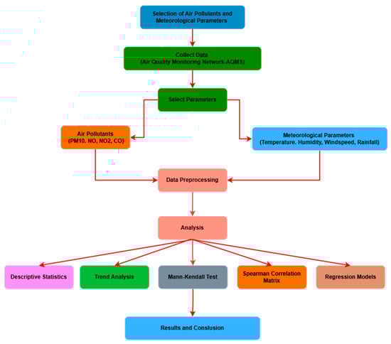
Figure 2.
Methodological workflow for the analysis of air pollutants and meteorological parameters.
3.2. Statistical and Machine Learning Methods
3.2.1. Descriptive Statistics
Descriptive statistics were employed to summarize the dataset, providing foundational insights into the central tendencies (mean, median), measures of dispersion (SD), and range (minimum, maximum) of the collected variables. This analysis included key air pollutants (PM10, NO, NO2, CO) and meteorological parameters (WS, temperature, RH, and RainF). By identifying baseline patterns, variability, and data distribution, this step facilitates subsequent analyses such as trend identification, correlation studies, and predictive modeling.
Descriptive statistics also play a crucial role in detecting potential outliers or anomalies that could impact the validity of further analyses. Outliers in environmental datasets, such as sudden spikes in pollutant levels, may indicate extraordinary events or measurement errors and need to be carefully evaluated. A detailed summary of the results is presented in Table 1 in the Results section, offering a comprehensive overview of pollutant concentrations and meteorological conditions during the study period.

Table 1.
Descriptive statistics of air pollutants (PM10, NO, NO2, CO) and meteorological parameters (WS, temperature, RH, RainF) measured in Sakarya city during 2021–2023.
3.2.2. Trend Analysis (Mann–Kendall Test)
The Mann–Kendall test, a widely used non-parametric statistical method, was applied to identify monotonic trends in air pollutant concentrations (PM10, NO, NO2, CO) across the study period (2021–2023). This method is particularly suited for environmental datasets characterized by non-normal distributions and seasonal variations, as it does not require assumptions about data distribution [26].
To complement the Mann–Kendall test, the Sen’s slope estimator was utilized to quantify the magnitude of any detected trends. The null hypothesis (H0) assumes no trend, while the alternative hypothesis (Ha) suggests a monotonic trend. A significance level (α) of 0.05 was employed to determine statistical significance.
This approach provides critical insights into the temporal dynamics of air quality, revealing whether pollutant levels are increasing or decreasing over time. Such trends are essential for assessing the effectiveness of emission control strategies and regulatory measures implemented in the study region. For example, a decreasing trend in NO2 concentrations may indicate the success of vehicular emission standards, while persistent PM10 levels could signal the need for additional interventions.
3.2.3. Correlation Analysis
Correlation analysis was performed to assess the relationships between air pollutants (PM10, NO, NO2, CO) and meteorological parameters (WS, temperature, RH, and RainF) over the study period. The Spearman correlation coefficient, a non-parametric measure of association, was selected due to its suitability for non-linear and non-normally distributed environmental datasets [27].
The Spearman coefficient ranges from −1 to 1:
- Positive values indicate a direct relationship.
- Negative values suggest an inverse relationship.
- Values near zero imply no significant association.
The preprocessed datasets were aligned across consistent time intervals to ensure robust and reliable results. Seasonal variations in correlations were also analyzed to capture how pollutant–meteorological relationships vary under different climatic conditions. For instance, WS was found to play a critical role in pollutant dispersion during winter, while RainF had a stronger influence on pollutant removal during spring and summer.
However, while Spearman correlation effectively identifies associations between variables, it does not infer causality. For example, a strong correlation between temperature and NO2 does not necessarily indicate a direct causal link, as other underlying factors (e.g., industrial emissions) may mediate this relationship. These limitations emphasize the need for complementary analyses to draw robust conclusions.
By identifying these relationships, the correlation analysis lays a strong foundation for predictive modeling, elucidating how meteorological factors influence pollutant behavior. These insights are crucial for designing targeted air quality management strategies and implementing evidence-based interventions to mitigate pollution effectively.
3.2.4. Regression Models
Regression models were utilized to assess the influence of meteorological parameters on air pollutant concentrations and to predict pollutant levels based on these variables. Two approaches were employed: MLR and RF regression. These methods were chosen to capture both linear and non-linear relationships, providing a comprehensive analysis of pollutant dynamics.
MLR
MLR is a statistical technique that models the relationship between a dependent variable (e.g., air pollutant concentration) and multiple independent variables (e.g., WS, temperature, RH, RainF). The model assumes a linear relationship and is expressed as:
where Ý represents the dependent variable (air pollutant concentration), while the independent variables—WS, TEMP, RH, and RainF—denote WS, temperature, RH, and RainF, respectively. α is the intercept, and the β coefficients represent the regression parameters of the model.
MLR provides insights into the linear contribution of each meteorological parameter to pollutant levels, enabling a straightforward interpretation of results. However, it may struggle to capture complex non-linear interactions.
Random Forest (RF) Regression
The random forest (RF) algorithm, first introduced by Breiman [28], is an ensemble learning method that improves decision trees through bagging (bootstrap aggregation) and random feature selection. It constructs multiple decision trees from bootstrapped subsets of the data, where each tree is trained using a randomly selected subset of features at each split. For classification, predictions are determined by majority voting, while for regression, they are averaged. This approach reduces overfitting, enhances generalization, and is robust to high-dimensional data. However, RF can be computationally expensive and less interpretable than single decision trees.
RF’s strength lies in its ability to handle large datasets, noisy features, and missing values while maintaining high accuracy. It inherently performs feature selection by considering only a subset of features at each split, reducing bias from dominant variables. Despite its advantages, RF requires careful tuning of hyperparameters like the number of trees and maximum depth to balance performance and efficiency. Its parallelizable nature makes it scalable, though inference can be slower due to the ensemble structure.
In addition, RF regression is a powerful machine learning algorithm that excels at capturing complex, non-linear relationships within datasets. Unlike traditional models such as MLR, RF does not assume a linear dependency between independent and dependent variables, making it particularly suited for environmental studies. These studies often involve intricate interactions between meteorological factors and air pollutant concentrations, which RF can model effectively.
At its core, RF operates as an ensemble method, leveraging the combined outputs of multiple decision trees to produce accurate and reliable predictions. This process begins with the random selection of subsets from the dataset, a technique known as bagging. Each decision tree in the ensemble is trained on a different subset, ensuring diversity and robustness. Additionally, at each split within a tree, a random subset of features is selected to prevent over-reliance on specific variables, further enhancing the model’s balance and generalizability [29].
Each decision tree is constructed by recursively splitting the data based on the feature that minimizes prediction error at each node. The trees are grown until a predefined stopping criterion, such as maximum depth or minimum node size, is met. Once all trees are built, their outputs are aggregated, typically by averaging in regression tasks, to generate final predictions. This ensemble approach reduces variance and improves the model’s ability to generalize to new data, making it particularly effective for datasets with high variability and complex relationships.
To address the common issue of overfitting, RF introduces randomness at multiple stages of its process. This, combined with its ensemble structure, significantly reduces the risk of overfitting, even when working with noisy or incomplete datasets. Another valuable feature of RF is its ability to evaluate the importance of input variables. By measuring each feature’s contribution to reducing prediction error, RF not only provides accurate predictions but also identifies key factors influencing pollutant concentrations, such as WS or RainF.
These strengths make RF a versatile and reliable tool for environmental modeling, providing both predictive power and critical insights into the dynamic interactions between meteorological parameters and air pollutants. Its robustness and adaptability ensure its effectiveness in addressing the complex challenges of air quality management.
The RF machine learning approach enhances temporal awareness by introducing lagged features for the variables, which are shifted by one time step. These lagged features help the model capture short-term patterns, such as pollutant buildup or weather effects, which improve pollutant prediction. Since RF does not inherently handle time, these engineered features add valuable context. Rows with missing values from the lagging process are then removed to ensure clean data for training.
Both MLR and RF models were trained using the dataset of air pollutants and meteorological parameters collected between 2021 and 2023. A rigorous technique for adjusting hyperparameters like “max_depth” and “n_estimators” 5-fold cross-validation, was used to optimize the model. In addition, cross-validation guarantees that the model does not overfit and that it performs effectively when applied to new data. The performance of these models was evaluated using the coefficient of determination (R2), which measures the proportion of variance in pollutant concentrations explained by the predictors. By combining the strengths of both models, this study provides a comprehensive understanding of how meteorological factors impact air pollutants. The insights gained contribute to the development of robust predictive models, which are essential for informed air quality management.
4. Results and Discussion
4.1. Descriptive Statistics and Analysis of Interactions Between Air Pollutants and Meteorological Parameters
Table 1 presents the descriptive statistics of air pollutants and meteorological parameters measured in Sakarya Province from 2021 to 2023. These metrics, including the minimum, maximum, mean, median, standard deviation (SD), and standard error (SE), offer critical insights into the temporal variability of pollutants and their interactions with meteorological conditions. The air pollutant values were measured independently and in absolute concentration, which is widely applied in similar environmental research [30,31].
Among the air pollutants, NO2 exhibited the highest mean concentration (32.4 ± 11.76 µg/m3), indicating persistent emission sources, such as traffic and industrial activities. Its moderate variability suggests seasonal fluctuations influenced by meteorological conditions like temperature and WS. PM10 concentrations showed significant variability (31.92 ± 16.24 µg/m3), reflecting diverse sources, including traffic, industrial emissions, and natural dust resuspension. The high SD highlights the combined influence of local sources and seasonal factors, such as dry weather or reduced RainF.
Carbon monoxide (CO) concentrations were relatively low (0.79 ± 0.39 mg/m3) and stable throughout the study period, with minimal seasonal variation. This stability suggests localized sources, such as residential heating and vehicular emissions, with limited long-range transport. Nitrogen monoxide (NO) displayed moderate variability (25.8 ± 19.35 µg/m3), primarily linked to traffic emissions. Its rapid conversion to NO2 likely explains its weaker correlation with meteorological parameters compared to other pollutants.
Meteorological parameters also exhibited variability, influencing pollutant dynamics. WS averaged 1.58 ± 0.59 m/s, significantly affecting the dispersion of pollutants. Higher WS values were associated with lower PM10 and NO concentrations, particularly during the winter and spring seasons. The mean temperature was 15.94 ± 7.02 °C, ranging from −1.7 °C to 29.1 °C, reflecting seasonal variations. Temperature played a critical role in pollutant dynamics by influencing chemical reactions and local emission sources, such as heating systems during colder months. RH averaged 72.06 ± 12.43%, with higher levels enhancing wet deposition and influencing atmospheric chemical transformations. RainF showed significant variability (2.30 ± 5.94 mm), contributing to the removal of particulate pollutants like PM10 through wet deposition, while having limited impact on gaseous pollutants such as NO and CO.
The substantial variability in PM10 concentrations underscores the need for targeted mitigation strategies, particularly during dry seasons when both natural and anthropogenic sources contribute to elevated levels. Similarly, the interplay between NO and NO2 highlights the critical role of traffic emissions and atmospheric chemical processes, emphasizing the necessity of addressing these pollutants collectively in air quality management.
Meteorological factors, particularly WS and RainF, demonstrated the most significant effects on pollutant levels, especially for PM10. These factors play a vital role in dispersing and removing pollutants from the atmosphere, thereby improving air quality. Conversely, the relative stability of CO concentrations suggests steady emissions from localized sources such as residential heating and vehicular activities, with minimal seasonal influence.
Overall, these findings emphasize the intricate interactions between air pollutants and meteorological parameters in Sakarya Province. Incorporating these meteorological factors into air quality assessments and predictive modeling is essential for a more comprehensive understanding of pollution dynamics and for guiding effective management strategies in urban–industrial environments.
4.2. Temporal Trends and Variations of Air Pollutants and Meteorological Parameters
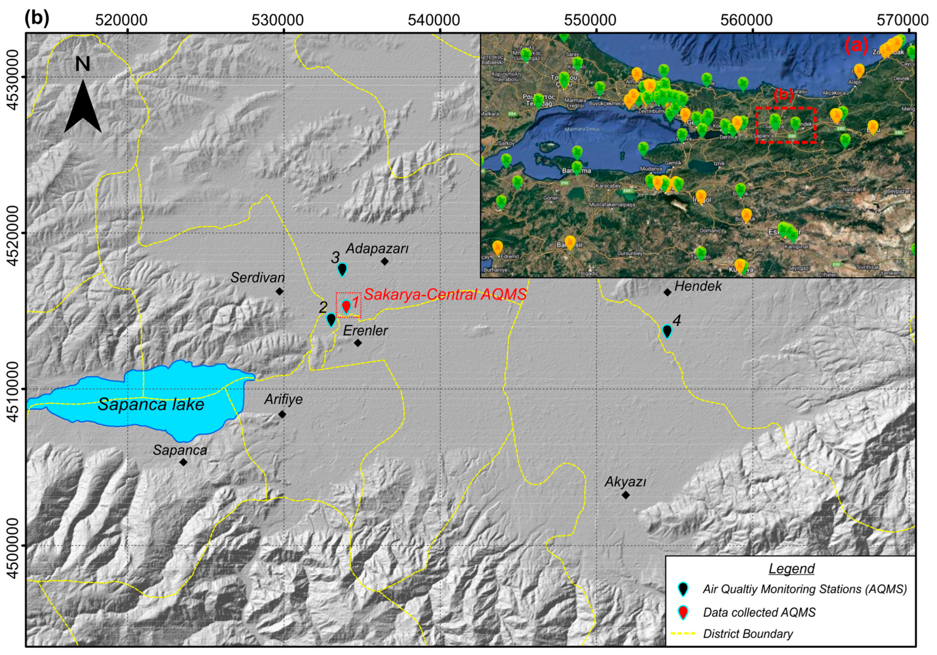
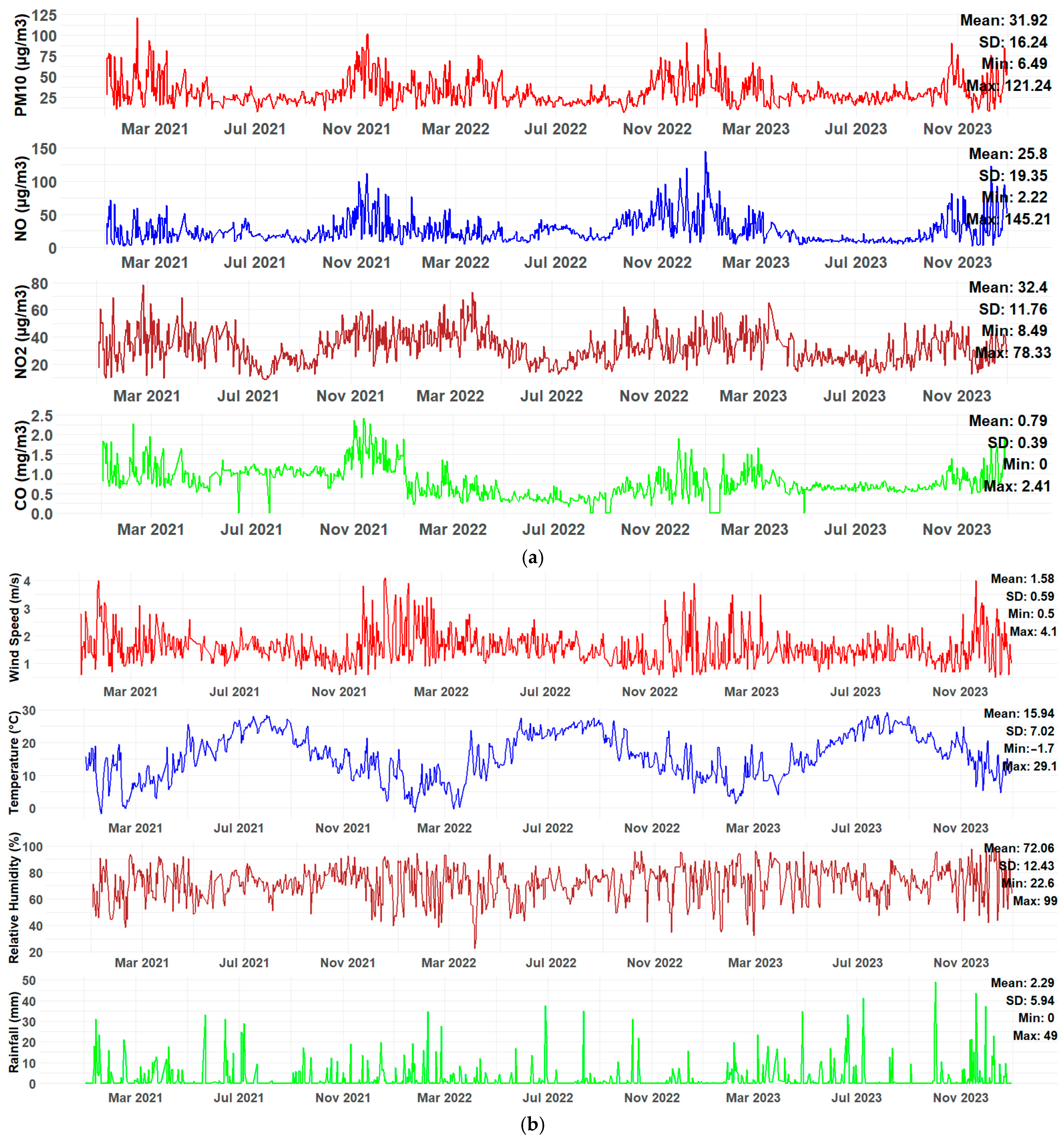
This study analyzed the temporal trends of air pollutant concentrations (PM10, NO, NO2, and CO) and meteorological parameters (WS, temperature, RH, and RainF) in Sakarya city between January 2021 and December 2023. The results, supported by Figure 3a–c and detailed statistical findings in Table 2, reveal critical insights into the dynamic interactions between air quality and meteorological conditions.
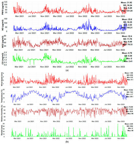
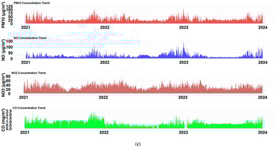
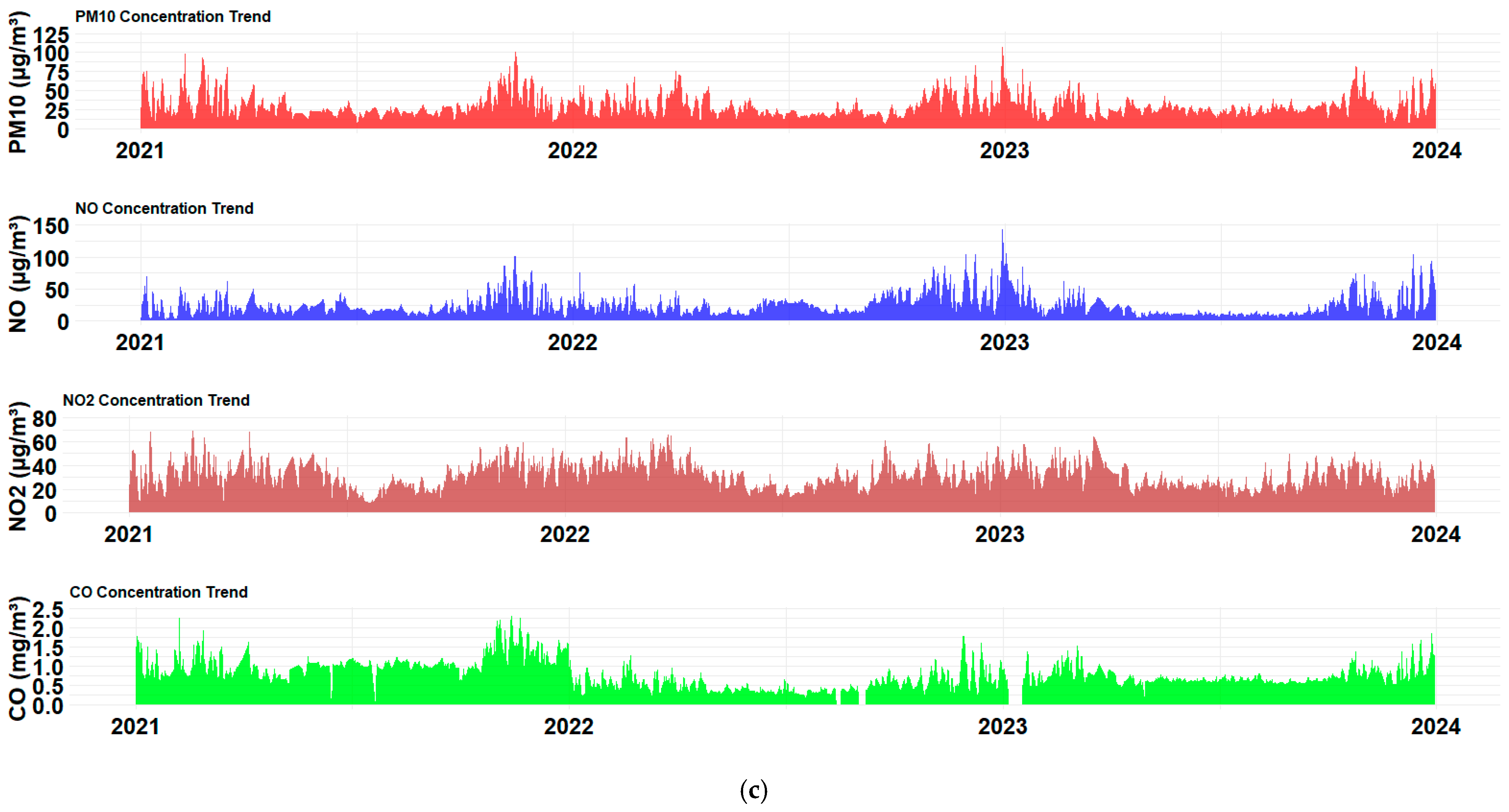
Figure 3.
(a) Seasonal trends of air pollutant concentrations (PM10, NO, NO2, and CO) in Sakarya (2021–2023); (b) seasonal trends of meteorological parameters (WS, temperature, RH, and RainF) in Sakarya (2021–2023); (c) comparative trends of PM10, NO2, NO, and CO concentrations in Sakarya (2021–2023).
Table 2.
Mann–Kendall trend analysis results for air pollutants (2021–2023).
The temporal trends of air pollutant concentrations are shown in Figure 3a. PM10 concentrations exhibited no statistically significant long-term trend (p = 0.97854, tau = 0.000563), indicating persistent sources such as traffic and industrial emissions without substantial mitigation over the study period. Similarly, NO displayed a negligible downward trend, which was not statistically significant (p = 0.25939, tau = −0.0235).
Conversely, NO2 concentrations showed a significant decline (p < 0.01, tau = −0.0879, Sen’s slope = −0.005354839), reflecting the effectiveness of emission control measures, particularly in reducing nitrogen oxides from vehicular traffic. CO concentrations experienced the steepest and most statistically significant reduction (p < 0.01, tau = −0.167, Sen’s slope = −0.0003175113), indicating successful interventions targeting carbon monoxide emissions from industrial and residential sources.
Meteorological parameters, illustrated in Figure 3b, exhibited clear seasonal variations. WS and temperature fluctuated in alignment with seasonal climatic patterns, averaging 1.58 m/s and 15.94 °C, respectively. RH (72.06%) and RainF (2.30 mm) peaked during wetter months, playing a critical role in pollutant dispersion, accumulation, and chemical transformations. WS significantly influenced pollutant dispersion, while RainF contributed to wet deposition, particularly for particulate matter like PM10.
The Mann–Kendall trend analysis, summarized in Table 2, confirmed these observations. Significant trends in NO2 and CO concentrations underscore the impact of stricter environmental regulations and technological improvements in emission control. On the other hand, the absence of significant trends in PM10 and NO highlights ongoing challenges in addressing these pollutants, particularly PM10, which originates from diverse sources such as vehicular emissions, industrial activities, and natural dust resuspension.
Figure 3c provides a comparative visualization of the temporal trends of NO2, NO, CO, and PM10 concentrations. The significant reductions in NO2 and CO concentrations reflect the success of emission control measures. In contrast, PM10 levels show subtle fluctuations with a slight upward tendency, emphasizing the need for enhanced strategies to address particulate matter pollution effectively.
The significant reductions in NO2 and CO concentrations demonstrate the success of emission control measures, while the persistence of PM10 levels underscores ongoing challenges in addressing particulate matter pollution. Targeted mitigation strategies, such as stricter industrial regulations and promoting public transport, are necessary to address PM10 effectively.
Meteorological factors, particularly WS and RainF, play a pivotal role in pollutant dispersion and removal processes. Integrating meteorological data into air quality assessments and adopting seasonally adaptive strategies is essential for effective air quality management in urban–industrial settings.
4.3. Model Comparison for Predicting Air Pollutant Concentrations
The performance of the MLR and RF models in predicting air pollutant concentrations (PM10, NO, NO2, and CO) based on meteorological parameters was compared. Table 3 summarizes the results using performance metrics such as R2, mean squared error (MSE), and root mean squared error (RMSE).
Table 3.
Comparative performance of RF and MLR models.
For PM10, the RF model demonstrated better performance, with an R2 value of 0.78 compared to 0.36 for MLR. RF also had a lower MSE (68.56 vs. 162.9) and RMSE (8.28 vs. 12.76). These results highlight RF’s ability to model non-linear interactions between PM10 and meteorological factors, such as WS and RainF. The findings also demonstrate superior performance compared to recent PM10 prediction efforts, achieving an R2 value of 0.38 [32] and 0.53 [33].
In the case of NO, RF outperformed MLR, with an R2 value of 0.71 versus 0.32, alongside lower MSE (139.48 vs. 217.6) and RMSE (11.81 vs. 14.75). This underscores RF’s effectiveness in capturing non-linearities in NO behavior. In addition, for NO2, RF slightly outperformed MLR, achieving an R2 of 0.65 compared to MLR’s 0.5. RF also reported marginally better error metrics, with lower MSE (49.14 vs. 67.7) and RMSE (7.01 vs. 8.23).
Both models struggled with CO prediction. RF achieved an R2 value of 0.39, slightly higher than MLR’s 0.18, but MSE (0.02) and RMSE (0.31) were identical for both models. The low predictive power aligns with research highlighting the challenges of modeling CO due to its diverse sources (e.g., traffic, industry, and residential heating) and weak correlations with meteorological variables. This indicates a need for advanced modeling approaches to improve CO predictions.
These results emphasize the importance of selecting appropriate models based on pollutant characteristics. RF performed better for PM10 NO, and NO2, which exhibit complex, non-linear relationships with meteorological parameters. The low predictive power for CO highlights the need for alternative approaches.
To improve prediction accuracy, future studies should consider incorporating additional data sources, such as emission inventories and chemical transformation mechanisms. Advanced modeling techniques, such as hybrid models or deep learning algorithms, could also be explored to better address pollutants with diverse and variable emission sources, particularly CO.
4.4. Seasonal Correlations Between Air Pollutants and Meteorological Parameters
The relationships between air pollutants (PM10, NO, NO2, and CO) and meteorological parameters (WS, temperature, RH, and RainF) were analyzed using the Spearman correlation matrix. The results, summarized in Table 4 and visualized in Figure 4, highlight significant seasonal variations influencing air pollutant concentrations. Additionally, Figure 5 provides detailed visualizations of seasonal variations in pollutant concentrations against meteorological parameters.
Table 4.
Seasonal Spearman correlation coefficients (r) between air pollutants and meteorological parameters (2021–2023).
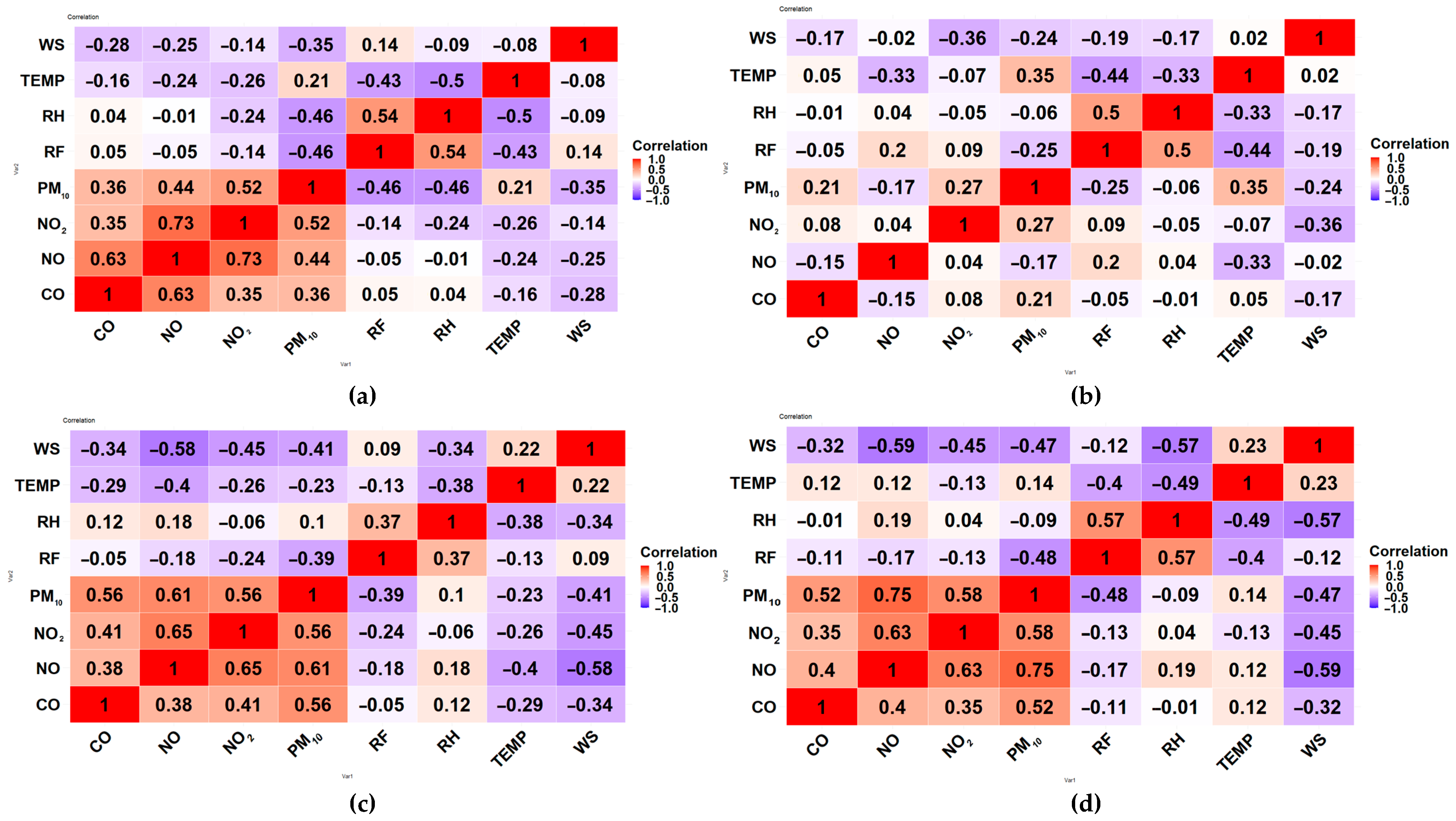
Figure 4.
Seasonal correlation matrix between air pollutants and meteorological parameters ((a): spring, (b): summer, (c): fall, (d): winter).
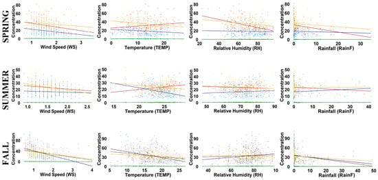
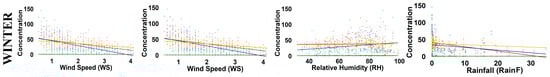
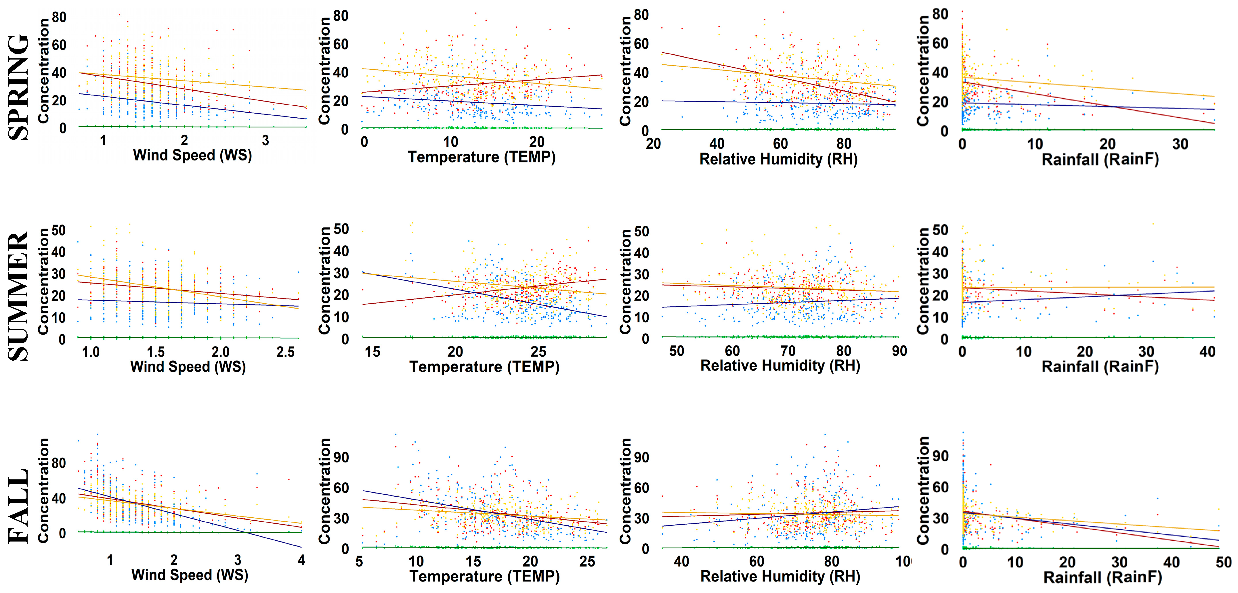
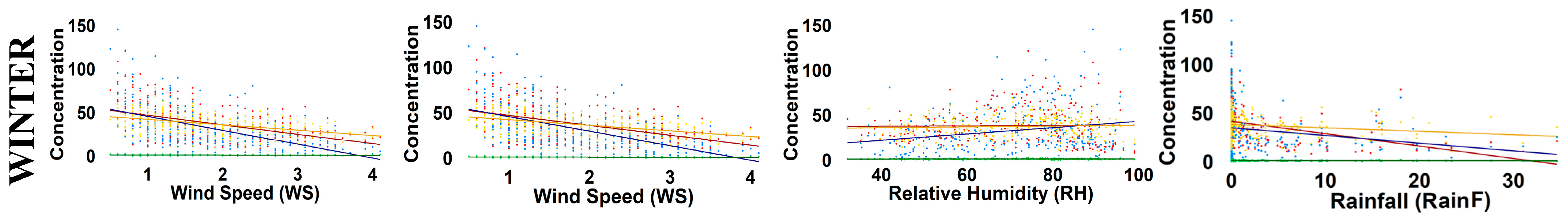
Figure 5.
Seasonal variation of pollutant concentrations against meteorological parameters. Colors represent the pollutants: dark red (PM10), navy blue (NO), dark goldenrod (NO2), and forest green (CO).
WS consistently exhibited a negative correlation with PM10, with the strongest impact observed during winter (r = −0.47) and fall (r = −0.41). These results highlight WS’s role in dispersing particulate matter, especially during colder months when atmospheric stability often limits natural dispersion. Similarly, WS showed strong negative correlations with NO in fall (r = −0.58) and winter (r = −0.59), further emphasizing its critical role in pollutant dispersion under stable atmospheric conditions. Conversely, its influence on NO2 and CO was minimal, reflecting these pollutants’ lower sensitivity to dispersion dynamics.
Temperature’s effect on pollutants varied by season. In summer, a moderate positive correlation with PM10 (r = 0.35) was observed, likely due to heightened emissions from industrial, agricultural, and vehicular activities during warmer months. In the fall, however, cooler temperatures led to moderate negative correlations with PM10 (r = −0.23) and NO (r = −0.40), as lower energy demands and reduced photochemical activity suppressed these pollutants. For NO2 and CO, temperature correlations remained weak and inconsistent across all seasons, suggesting a more complex or indirect relationship.
RH exhibited dual effects depending on the season. In spring, RH negatively correlated with PM₁₀ (r = −0.46), likely due to enhanced wet deposition. However, in fall and winter, RH showed weak positive correlations with NO (r = 0.18 and r = 0.19, respectively), potentially promoting nitrogen oxide accumulation in colder, more humid conditions. These seasonal shifts underline RH’s dual role in both pollutant removal and atmospheric chemical transformations.
RainF emerged as a key factor in pollutant reduction, showing a consistent negative correlation with PM10 across all seasons, with the strongest effects in winter (r = −0.48) and spring (r = −0.46). This underscores RainF’s effectiveness in particulate matter removal via wet deposition. For NO, a weak positive correlation was observed in summer (r = 0.20), likely due to localized emission patterns, while its influence on NO2 and CO was negligible.
The analysis highlights WS and RainF as the most influential meteorological parameters in reducing PM10 and NO concentrations, particularly in colder and wetter seasons. Meanwhile, temperature and RH exhibited complex, pollutant-specific effects that varied by season.
These findings emphasize the necessity of incorporating seasonal meteorological data into air quality management strategies. By addressing pollutant-specific challenges and adapting to seasonal variations, more effective mitigation measures can be implemented, improving air quality in urban and industrial regions.
5. Conclusions
This study explored the seasonal dynamics of key air pollutants (PM10, NO, NO2, and CO) and their relationships with meteorological parameters (WS, temperature, RH, and RainF) in Sakarya city from 2021 to 2023. The findings emphasize the critical roles of WS and RainF in reducing PM10 and NO levels, particularly through wet deposition and atmospheric dispersion. While RF outperformed MLR in capturing non-linear pollutant-meteorological interactions, the models struggled to predict CO concentrations due to its localized sources and weak meteorological dependencies. Temperature and RH exhibited complex, pollutant-specific effects, with PM10 showing increased levels during summer but reduced levels under humid spring conditions. These results underscore the intricate interplay between meteorological factors and air pollutant dynamics, providing actionable insights for data-driven air quality management.
This study is limited by its focus on Sakarya, Türkiye, which may restrict the generalizability of its findings to other regions with different geographic, climatic, and emission characteristics. Additionally, the accuracy of the results depends on the availability and quality of air pollution and meteorological data, as any gaps or inconsistencies in the dataset could affect model performance. The study’s temporal scope may also limit its ability to capture long-term trends or the impacts of extreme environmental events and policy changes on air quality.
The study highlights the necessity of incorporating meteorological data into air quality assessments and developing seasonally adaptive, pollutant-specific strategies. To address persistent PM10 emissions and the challenges associated with CO prediction, stricter industrial and vehicular emission regulations, along with advanced hybrid modeling approaches, are essential. Furthermore, integrating renewable energy adoption, real-time monitoring systems, and green urban planning can significantly enhance air quality in urban–industrial regions like Sakarya. Future research should expand the scope to include long-term analyses, detailed emission inventories, and cross-regional comparisons to validate these findings and identify scalable solutions. These efforts will contribute to a more comprehensive understanding of air pollution dynamics and the development of effective, sustainable mitigation strategies.
Author Contributions
Conceptualization, B.E.; methodology, B.E.; software, B.E. and S.S.; validation, B.E. and S.S.; formal analysis, B.E. and S.S.; investigation, B.E.; resources, B.E. and S.S.; data curation, Y.D.A.; writing—original draft preparation, S.S.; writing—review and editing, B.E. and S.O.; visualization, S.S.; supervision, B.E.; project administration, B.E. and S.S.; funding acquisition, B.E. All authors have read and agreed to the published version of the manuscript.
Funding
This research was funded by the Sakarya University Scientific Research Projects Coordination Unit (SAÜ BAP), grant number 2024-25-59-139.
Data Availability Statement
Restrictions apply to the availability of these data. Data were obtained from Provincial Directorate of the Ministry of Environment, Urbanization, and Climate Change and and Sakarya Meteorological Office and are available from the authors with the permission of Provincial Directorate of the Ministry of Environment, Urbanization, and Climate Change and Sakarya Meteorological Office.
Conflicts of Interest
The authors declare that the research was funded by the Sakarya University Scientific Research Projects Coordination Unit (SAÜ BAP), which may cause potential conflicts of interest.
Abbreviations
The following abbreviations are used in this manuscript:
| MLR | Multiple Linear Regression |
| MSE | Mean Squared Error |
| R2 | Coefficient of Determination |
| RainF | Rainfall |
| RF | Random Forest |
| RH | Relative Humidity |
| RMSE | Root Mean Squared Error |
| SD | Standard Deviation |
| SE | Standard Error |
| Temp | Temperature |
| WS | Wind Speed |
References
- Meng, Y.; Liu, Z.; Hao, J.; Tao, F.; Zhang, H.; Liu, Y.; Liu, S. Association between ambient air pollution and daily hospital visits for cardiovascular diseases in Wuhan, China: A time-series analysis based on medical insurance data. Int. J. Environ. Health Res. 2022, 33, 452–463. [Google Scholar] [CrossRef]
- Dandotiya, B. Air Pollution, Health and Perception; IntechOpen: London, UK, 2021. [Google Scholar] [CrossRef]
- Mbaoma, O.; Ogunkeyede, A.; Adebayo, A.; Otolo, S.; Ikpinima, M. Geostatistical analysis for monitoring and modelling atmospheric pollutants. J. Geogr. Environ. Earth Sci. Int. 2022, 26, 46–57. [Google Scholar] [CrossRef]
- He, S.; Li, Z.; Wang, W.; Yu, M.; Liu, L.; Alam, N.; Gao, Q.; Wang, T. Dynamic relationship between meteorological conditions and air pollutants based on a mixed copula model. Int. J. Climatol. 2021, 41, 2611–2624. [Google Scholar] [CrossRef]
- Cai, X.; Yu, J.; Qin, Y. Spatial distribution of air pollution and its relationship with meteorological factors: A case study of 31 provincial capitals in China. Pol. J. Environ. Stud. 2023, 32, 2513–2521. [Google Scholar] [CrossRef]
- Gao, R.; Wang, B.; Huang, S. Impacts of meteorological conditions on PM2.5 and PM10 pollution in Zhengzhou, China. E3S Web Conf. 2021, 257, 03025. [Google Scholar] [CrossRef]
- Yang, Q.; Yuan, Q.; Li, T.; Shen, H.; Zhang, L. The relationships between PM2.5 and meteorological factors in China: Seasonal and regional variations. Int. J. Environ. Res. Public Health 2017, 14, 1510. [Google Scholar] [CrossRef]
- Shi, H.; Critto, A.; Torresan, S.; Gao, Q. The temporal and spatial distribution characteristics of air pollution index and meteorological elements in Beijing, Tianjin, and Shijiazhuang, China. Integr. Environ. Assess. Manag. 2018, 14, 710–721. [Google Scholar] [CrossRef]
- Bodor, Z.; Bodor, K.; Keresztesi, Á.; Szép, R. Major air pollutants seasonal variation analysis and long-range transport of PM10 in an urban environment with specific climate condition in Transylvania (Romania). Environ. Sci. Pollut. Res. 2020, 27, 38181–38199. [Google Scholar] [CrossRef]
- Okimiji, O.; Techato, K.; Simon, J.; Tope-Ajayi, O.; Okafor, A.; Aborisade, M.; Phoungthong, K. Spatial pattern of air pollutant concentrations and their relationship with meteorological parameters in coastal slum settlements of Lagos, Southwestern Nigeria. Atmosphere 2021, 12, 1426. [Google Scholar] [CrossRef]
- Wang, J.; Gao, J.; Che, F.; Yang, X.; Yang, Y.; Liu, L.; Xiang, Y.; Li, H. Summertime response of ozone and fine particulate matter to mixing layer meteorology over the North China Plain. Atmos. Chem. Phys. 2023, 23, 14715–14733. [Google Scholar] [CrossRef]
- Huang, F.; Li, X.; Wang, C.; Xu, Q.; Wang, W.; Luo, Y.; Tao, L.; Gao, Q.; Guo, J.; Chen, S.; et al. PM2.5 spatiotemporal variations and the relationship with meteorological factors during 2013–2014 in Beijing, China. PLoS ONE 2015, 10, e0141642. [Google Scholar] [CrossRef] [PubMed]
- Liu, Y.; Zhou, Y.; Lu, J. Exploring the relationship between air pollution and meteorological conditions in China under environmental governance. Sci. Rep. 2020, 10, 14518. [Google Scholar] [CrossRef] [PubMed]
- Qiao, Z.; Wu, F.; Xu, X.; Yang, J.; Liu, L. Mechanism of spatiotemporal air quality response to meteorological parameters: A national-scale analysis in China. Sustainability 2019, 11, 3957. [Google Scholar] [CrossRef]
- Rahman, M.; Wang, S.; Zhao, W.; Xu, X.; Zhang, W.; Arshad, A. Investigating the relationship between air pollutants and meteorological parameters using satellite data over Bangladesh. Remote Sens. 2022, 14, 2757. [Google Scholar] [CrossRef]
- Hou, K.; Xu, X. Evaluation of the influence between local meteorology and air quality in Beijing using generalized additive models. Atmosphere 2021, 13, 24. [Google Scholar] [CrossRef]
- Yan, S.; Cao, H.; Chen, Y.; Wu, C.; Hong, T.; Fan, H. Spatial and temporal characteristics of air quality and air pollutants in 2013 in Beijing. Environ. Sci. Pollut. Res. 2016, 23, 13996–14007. [Google Scholar] [CrossRef]
- Xu, Y.; Xue, W.; Lei, Y.; Zhao, Y.; Cheng, S.; Ren, Z.; Huang, Q. Impact of meteorological conditions on PM2. 5 pollution in China during winter. Atmosphere 2018, 9, 429. [Google Scholar] [CrossRef]
- Park, S.; Sabbah, I.; Kwak, H.; Prasad, A.; Lee, W.; Kafatos, M. Studying air pollutants origin and associated meteorological parameters over Seoul from 2000 to 2009. Adv. Meteorol. 2015, 2015, 704178. [Google Scholar] [CrossRef]
- Eduk, A.; Leo, C.; Andrew, A.; Mudiaga, C. Prediction and modeling of dry seasons air pollution changes using multiple linear regression model: A case study of Port Harcourt and its environs, Niger Delta, Nigeria. Int. J. Environ. Agric. Biotechnol. 2018, 3, 899–915. [Google Scholar] [CrossRef]
- Liang, P.; Zhu, T.; Fang, Y.; Li, Y.; Han, Y.; Wu, Y.; Hu, M.; Wang, J. The role of meteorological conditions and pollution control strategies in reducing air pollution in Beijing during APEC 2014 and Victory Parade 2015. Atmos. Chem. Phys. 2017, 17, 13921–13940. [Google Scholar] [CrossRef]
- Zhang, Z.; Ma, N. Research on air quality prediction method based on GA-BP model. In Proceedings of the International Conference on Computer Application and Information Security (ICCAIS 2021), Wuhan, China, 18–19 December 2021; SPIE: Bellingham, WA, USA, 2022; Volume 12260, pp. 345–359. [Google Scholar] [CrossRef]
- Liu, W.; Li, X.; Chen, Z.; Zeng, G.; León, T.; Liang, J.; Huang, G.; Gao, Z.; Jiao, S.; He, X.; et al. Land use regression models coupled with meteorology to model spatial and temporal variability of NO2 and PM10 in Changsha, China. Atmos. Environ. 2015, 116, 272–280. [Google Scholar] [CrossRef]
- Choi, S.M. Improved Air Quality Forecasting-Based on Machine Learning and Multivariate Regression Techniques. Interciencia 2024, 35, 2–19. [Google Scholar] [CrossRef]
- Choi, S.M. Assessment of Improved Artificial Neural Network Models for Urban Air Quality Forecasting by Transboundary Pollutants. Interciencia 2025, 36, 47–67. [Google Scholar] [CrossRef]
- Malhotra, M.; Aulakh, I. Meteorological factors correlation with air pollutants: A case study in Delhi. Int. J. Environ. Sci. Dev. 2023, 14, 91–105. [Google Scholar] [CrossRef]
- Vani, P.C.; Sahoo, B.C.; Paul, J.C.; Sahu, A.P.; Mohapatra, A.K.B. Trend analysis in gridded rainfall data using Mann-Kendall and Spearman’s Rho tests in Kesinga Catchment of Mahanadi River Basin, India. Pure Appl. Geophys. 2023, 180, 4339–4353. [Google Scholar] [CrossRef]
- Breiman, L. Random forests. Mach. Learn. 2001, 45, 5–32. [Google Scholar] [CrossRef]
- Zheng, Y.; Meng, Y.; Lou, E.; Li, Y. Analysis of global temperature influencing factors based on Spearman correlation coefficient method and grey correlation theory. Highlights Sci. Eng. Technol. 2023, 48, 102–111. [Google Scholar] [CrossRef]
- Yang, Y.; Mei, G.; Izzo, S. Revealing influence of meteorological conditions on air quality prediction using explainable deep learning. IEEE Access 2022, 10, 50755–50773. [Google Scholar] [CrossRef]
- Bose, A.; Roy Chowdhury, I. Investigating the association between air pollutants’ concentration and meteorological parameters in a rapidly growing urban center of West Bengal, India: A statistical modeling-based approach. Model. Earth Syst. Environ. 2023, 9, 2877–2892. [Google Scholar] [CrossRef]
- Cabello-Torres, R.J.; Estela, M.A.P.; Sánchez-Ccoyllo, O.; Romero-Cabello, E.A.; Ávila, F.F.G.; Castañeda-Olivera, C.A.; Valdiviezo-Gonzales, L.; Eulogio, C.E.Q.; Cruz, A.R.H.D.L.; López-Gonzales, J.L. Statistical modeling approach for PM10 prediction before and during confinement by COVID-19 in South Lima, Perú. Sci. Rep. 2022, 12, 16737. [Google Scholar] [CrossRef]
- Mamić, L.; Gašparović, M.; Kaplan, G. Developing PM2.5 and PM10 prediction models on a national and regional scale using open-source remote sensing data. Environ. Monit. Assess. 2023, 195, 644. [Google Scholar] [CrossRef] [PubMed]

Disclaimer/Publisher’s Note: The statements, opinions and data contained in all publications are solely those of the individual author(s) and contributor(s) and not of MDPI and/or the editor(s). MDPI and/or the editor(s) disclaim responsibility for any injury to people or property resulting from any ideas, methods, instructions or products referred to in the content. |
© 2025 by the authors. Licensee MDPI, Basel, Switzerland. This article is an open access article distributed under the terms and conditions of the Creative Commons Attribution (CC BY) license (https://creativecommons.org/licenses/by/4.0/).