Abstract
EU Directive 49/2002 and Spanish law 37/2006 urge cities to develop strategic noise maps and action plans to evaluate noise exposure and to establish noise abatement procedures in critical areas. However, noise mapping involves costly and cumbersome measurement procedures that can become a real issue in practice. This paper describes a distributed noise monitoring system based on WASN (Wireless Acoustic Sensor Network) and the application of a geo-statistical methodology for statistical spatial-temporal prediction of noise levels in semi-open areas, such as a typical, small Mediterranean city (Algemesí, València, Spain). This methodology is applied to the study of the spatial evolution in time of the noise pollution. To this end, a spatial statistical model is developed by using the noise pollution measurements obtained over a set of points located at some strategic locations. The geo-statistical time model allows for estimating specific noise levels and characterizing the spatial-temporal variation of the noise pollution. The results show that the developed model provides a good approximation of the measurements obtained experimentally.
1. Introduction
Real-time mapping systems for noise pollution monitoring is a challenging issue that has already been addressed in several research works [1,2]. In this context, the study of noise pollution in urban environments aimed at developing networked monitoring systems combined with spatial models for predicting sound pressure levels is not straightforward.
Noise pollution is a common problem in urban environments. It affects human behavior, health and even children’s cognition. Recognizing this as a major issue, the European Commission adopted a directive [3], requiring main cities (with more than 100,000 inhabitants) to gather real world data on noise exposure in order to produce local action plans and to provide accurate mappings of noise pollution levels. The traditional way of conducting noise measurements is by collecting noise samples manually, but this technique has many drawbacks. On the one hand, only local and sparse measurements are taken. On the other hand, it is expensive due to the measuring equipment and personnel costs.
However, the European Commission recommends for higher granularity of noise data both in space and time. In this scenario, Wireless Sensor Networks (WSNs) represent an alternative that can overcome the drawbacks of the current noise data collection procedure. These WSNs are composed of small autonomous nodes with sensing capabilities. Each node has its own power supply, processing unit and memory. The nodes communicate using multi-hop routing protocols and at least one node (named sink) acts as a gateway for external connection. In the last decade, several studies have been conducted using WSN for noise pollution monitoring. All of these studies are based on the equivalent sound pressure level over time T.
Several works have considered the use of WASNs for noise monitoring. In [4,5], authors have evaluated a WASN using Tmote-Sky motes [6] and Tmote Invent (TmI), to monitor traffic noise using the equivalent level, and to count the number and type of vehicles. In this deployment, they used a sampling frequency of 8 kHz. In their study, they found that Tmote-Sky had excessive self-noise and TmI (with an integrated microphone) had apparently good audio features. In the references, the authors do not provide a specific calibration.
In [7,8], a WASN deployment in Ostrobothnia (Finland) is discussed. In these references, the authors report different tests to evaluate the noise impact. They measured the with ms using a sampling frequency of 33 kHz, with 14 calibrated motes (MicaZ from Crossbow -now this company is MEMSIC- with an ad hoc acquisition circuitry to allow a dynamic range of 60 dB), globally synchronized during 96 h with good results.
Other references such as [1,9,10] have used mobile phones for noise pollution monitoring. Although the results are interesting, in our opinion, there is a lack of information about the recording conditions which avoids getting accurate noise measurements. When evaluating noise parameters, the location of the measuring devices should follow specific rules [3].
In all of the previous references [1,4,5,6,7,8,9,10], the measurements are based on the or its A-weighted version (ITU-R 468), . These measurements apply a frequency-selective filter that picks up the frequency range around 3–6 kHz, where the human ear is most sensitive. These parameters are measured in dB and dBA, respectively.
The data collection procedure from the sensor nodes must also be considered. In the literature [11], there are several approaches that allow a good data collection. These protocols are associated not only to the routing protocols of the information to the sink, but also to the application to represent the information which can be presented as a web-service.
Another issue to consider in the data information system is the statistical representation of the noise data information oriented to detect problematic areas in real time. A promising tool for this kind of noise mapping is given by geo-statistics, which provides a set of statistical techniques specifically designed for spatial problems. These methods are aimed at predicting the values of a certain phenomenon over an area where several points have been sampled [12]. The predictions are based on statistical models that can incorporate additional information as explicative variables. Moreover, the prediction error can be estimated using uncertainty propagation [13,14].
The use of an equally distributed sampling grid allows for a better determination of the mean value for the underlying statistical distribution of the sampled data obtained at the measuring points. For this reason, the use of geostatistical interpolation, as performed by the Ordinary Kriging (OK) method [12], can be applied, since the mean value of the measured distribution is already known.
The goal of this paper is to analyze the suitability of a hardware system for noise measuring, based on Raspberry Pi nodes with a condenser microphone as an acoustic sensor and a data collection system, combined with geo-statistical techniques which are applied to the problem of noise mapping in a small city in the Valencian Community in Spain. The advantages provided by geographic information systems (GIS) are also used to locate precisely the measurement locations within a heterogeneous environment. A predictive model is developed by analyzing the noise pollution measurements obtained from a small set of points over a specific city. This model allows for obtaining punctual level estimates and calculating the spatial-temporal variation of the noise pollution level. To this end, the OK interpolation method will be considered. The main objective of this paper is then to evaluate the performance of the Wireless Acoustic Sensor Network (WASN) in combination with this spatial-temporal interpolating method at estimating the values corresponding to unsampled spatial locations, provided that the sampling grid has been correctly designed. This applied study is oriented to find the noise climate in different points for predicting global behaviors. As a result, the method allows for establishing environmental local policies for noise control and zonification at a municipal level, evaluating the local impact of the sound sources.
2. Material and Method
Before describing the developed monitoring system and the spatial statistical predictive model and its application, some notes about the place, the network and the measurements are next given.
2.1. The City
The measurements were carried out in Algemesí (Valencia, Spain). This is a small city with 28,000 inhabitants, located at the South-East of Valencia at coordinates N 9.12 W 0.12. The city is in an agricultural area, although an incipient industrial sector is also growing. The Magre River, which is an affluent of the Xuquer River, flows in the NW-SE of the town settling a natural border.
2.2. The Network
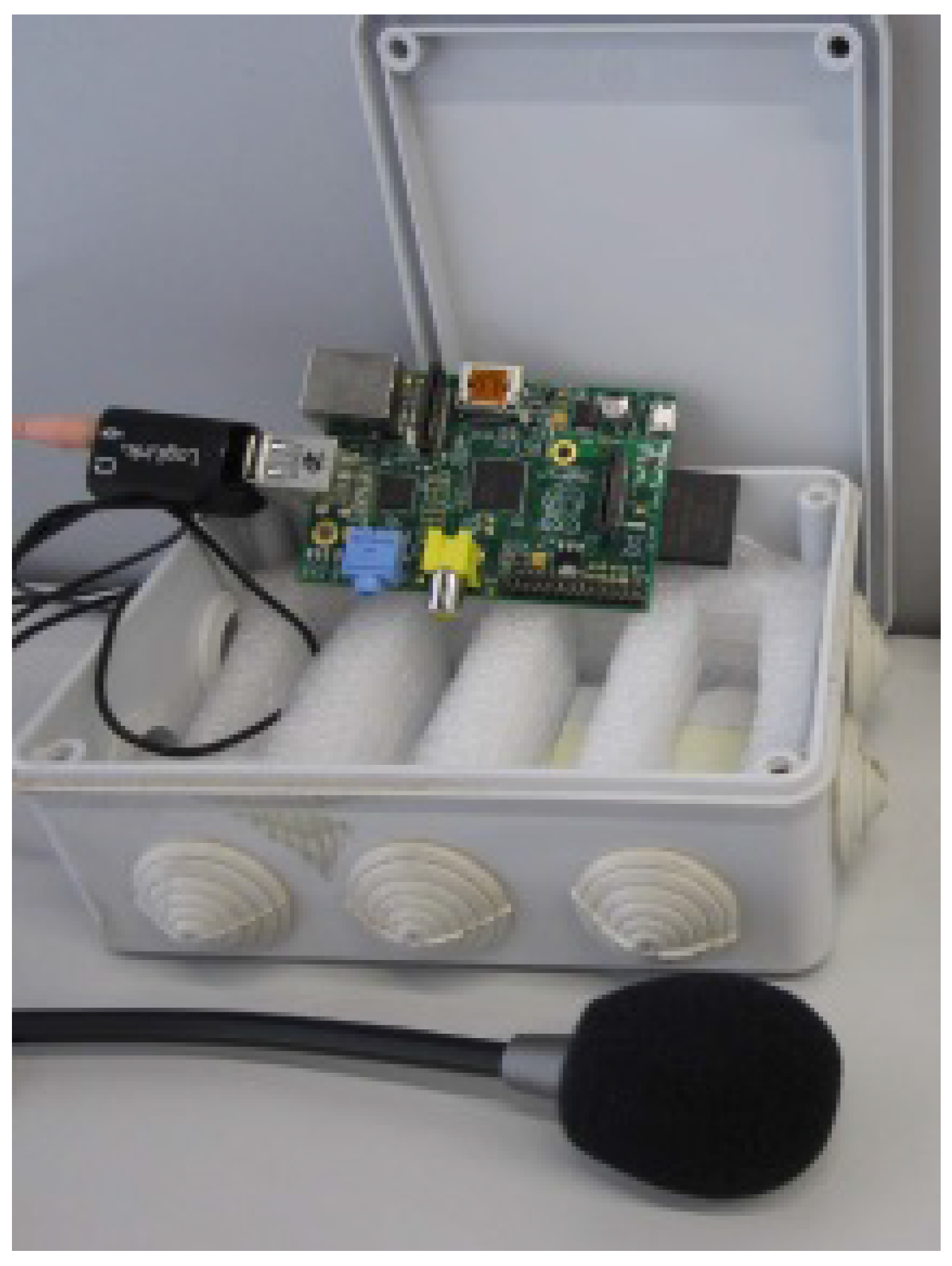
The used nodes in the network are based on Raspberry Pi B (RPi) platform. This platform is based on Broadcom BCM2835 System-on-Chip (SoC) [15], including an ARM1176JZF-S 700 MHz processor [16], a Graphic Processing Unit (GPU) and 512 MB of RAM, with a SD slot card memory. A Logilink UA0053 USB sound card [17] was installed in the RPis in order to record the audio, with an electret omnidirectional microphone [18]. The frequency response of the electret microphone is nearly flat from 60-16000KHz. Also a WiFi adapter TP-Link TL-WN725N [19] with IEEE 802.11 b/g/n standard has been introduced in the setup for communication purposes. This configuration allows each node to acquire several seconds of audio with 16 bits per sample (allowing a dynamic range of dB) at a sampling frequency of 22.05 kHz. The RPi have been placed in a protective housing, each with 3 Kodak 1.5 V KDLR20 batteries (19,500 mAh) [20]. A mean current consumption of 550 mAh (5 V) was measured, by disabling all unnecessary services in the operating system. It allows a life-time of 28 hours, considering an 80% efficiency for the batteries.
A Raspbian Operating System [21] was installed in the RPi, which is a GNU/Linux version optimized for RPi hardware, based on a Debian distribution. To implement a Wireless Mesh Network, the Babel [22] routing protocol was used. This is a loop free, proactive protocol and it is based on distance vector algorithm. Babel is implemented in the Quagga [22] software suite. Also, a Cloud client called OwnCloud [23] was installed in each node, in order to gather the information from the different sensors into one system, connected to the Internet. The Owncloud server application was installed in a PC. This system allows storing and automatic synchronization of the information from the different nodes spatially distributed.
A batch script has been programmed in order to setup an automatic measurement for 10 min [24,25] every 3 h in each node. This allows a synchronized measurement within the established network. Figure 1 shows an RPi node with the electret microphone outside the box.
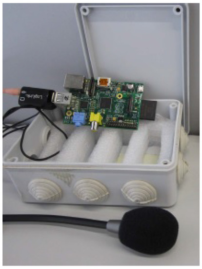
Figure 1.
Measurement node setup.
Finally, a web-service based on OpenCPU [26] has been installed on a web server. This web-service allows programming in R. Its purpose is to harvest data from the cloud and process it using spatial statistics as explained later. Figure 2 shows the result of the node 4 (see location in Figure 3).
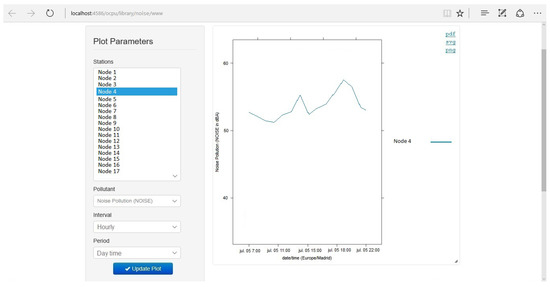
Figure 2.
OpenCPU framework to gather the noise pollution information.
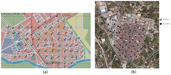
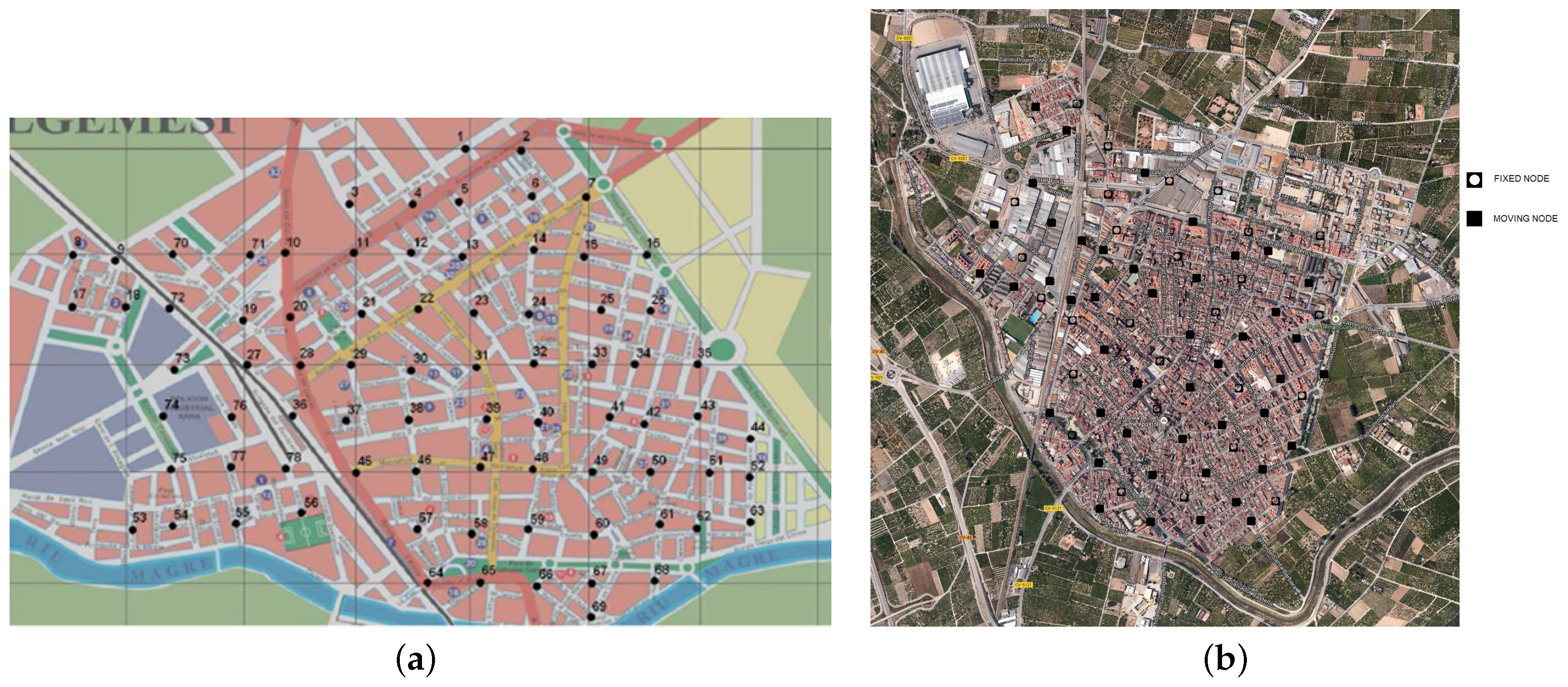
Figure 3.
Location of the measurement points for the plan of Algemesí (a); fixed nodes and moving nodes (b).
In order to validate the sonometric records obtained with the RPi, a calibrated Type I standard sound level meter (CESVA SC-310 [27]) has been used to calibrate and check the different measurements at the same time of the calibrating experiments. Using previously digital recorded audio files of road traffic in one of the locations the mean and standard deviation of the during a 10 min period have analyzed. Before setting up the network test, a standard calibration using piston phones has been performed, to avoid the misalignment in the measured parameters due to the mismatches in microphones’ sensitivities and frequency responses. The measurements were compared with the standard sound level meter and showed less than dB error, both in short-term and long-term measures. This difference has been considered to adjust the values of the on-site measurements.
2.3. The Measurements
The measurements were carried out following a grid over an urban plan of the city, in an extension of 1.80 km. The measurements were conducted at 78 positions as shown in the map of Figure 3. The measurement set was divided into periods of 3 hours, covering the diurnal period from 07:00 h to 22:00 h. Each location has one measurement in every regular temporal interval. A total of 390 measurements were obtained for performing the statistical analysis. The measurements were taken simultaneously by using a network with 39 RPi nodes measuring during 10 minutes in each time period. These measurements were taken in three weeks. Some of the nodes (27) were located in fixed places. The rest (12 nodes) were used as moving nodes, but immovable while measuring, in order to cover all the measuring network. Figure 3a shows the locations of all the measurement points in the urban area. The fixed nodes are shown in Figure 3b as hollowed squares and the moving nodes as filled squares. These moving nodes have been changed during the three weeks that lasted the experiment in order to record sound levels in all the day-time periods for every measuring location.
In the measurement places, traffic noise is recognized as one of the major contributors to the environmental noise [28]. Therefore, traffic conditions during the measurement period should be also conveniently reported when conducting the measurements. Information on the number and vehicle types (light/heavy vehicles or motorcycles) was gathered in the measuring nodes, as well as their average speed and the kind of pavement on the road (asphalt, concrete, paving stones or soil). This information has been gathered by configuring RPi camera [29] and storing the video (coded using QCIF resolution and H.263) at the same folder in the Cloud using the same time as the noise measurement in each node for each time period. It is important to note that the physical characteristics of the environment and the presence of animals or people speaking can also influence the noise level. This information is reflected in a set of qualitative or quantitative variables, as summarized in Table 1.

Table 1.
Variables used.
2.4. Descriptive analysis of the data
The measurement process, especially its temporal distribution, leads us to 5 equally distributed time slots covering the diurnal period from 07:00 h to 22:00 h. For each of these time slots, there are 78 samples available, one per measurement location. Table 1 describes the information gathered by each node.
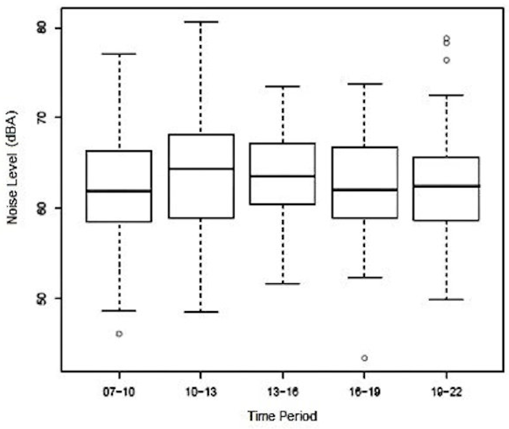
Table 2 and Figure 4 show the results of the descriptive analysis of the noise level in these five temporal periods. The values in Table 2 and the box diagrams suggest the invariance of the mean value in the measured data, whose results are shown in Table 3.

Table 2.
Descriptive statistics of noise levels in different time periods.

Figure 4.
Box diagram of the measurements.

Table 3.
ANOVA (Analysis of Variance) of noise levels in different time periods.
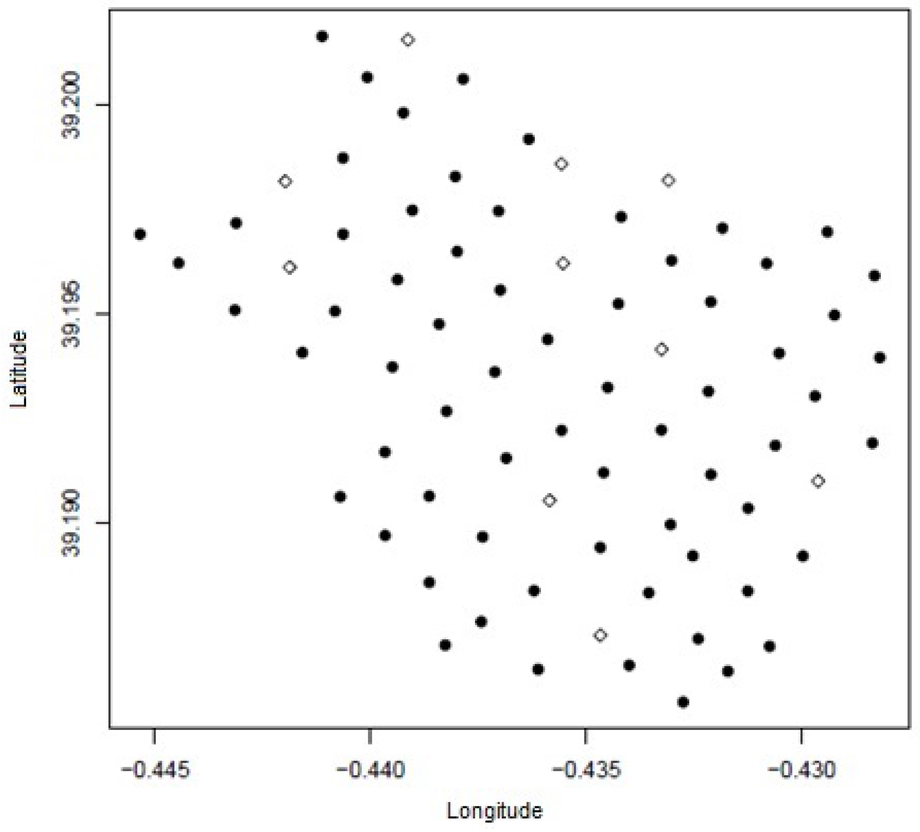
The 78 locations are divided into two sets in order to check the validity of the proposed models: a modelling set, composed of 68 locations and a validation set, which has 10 locations. Both sets are used for all of the time periods and are shown in Figure 5. In order to select the nodes of the validation set, a distribution that bounds the semivariogram error has been chosen, so the nodes are spatially distributed throughout the whole area.

Figure 5.
Modelling set (black dots); and validation set (white dots).
2.5. Spatial Analysis
The obtained noise pollution measurements constitute a data set linked to several locations with its geographical coordinates, longitude and latitude. By denoting the acoustic noise level at a location x as , we can define this data set as , where are all the locations of the modeling set (68 positions).
In this context, the objective of our model is the prediction of in any location , particularly those in the validation set. The noise reports contain information (as shown in Table 1) of the set of covariables included. Consequently, is modeled as a tendency function of the influencing covariables in the process that explains its variability in a large extent plus some random error explaining the short term variability, i.e.,
where and is a Gaussian process intrinsically stationary with zero mean, whose spatial dependence characterization is given by the variogram [30]:
where denotes the variance and h is an offset. In this study, the variogram has been calculated with the R statistical package for variogram fitting [31].
3. Results and Discussion
Several studies [28,32,33] conclude that is the covariable that better explains the noise level, where Q is the total number of vehicles. This coincides with other studies [34,35] on noise pollution in close urban areas. In this case, the variable seems to be the determinant element for the noise level in the city, and it is a significant covariable in all of the time periods. These covariables have been analyzed separately in each one of the five time periods. However, other variables could have a significant impact in any of the time periods, although less important than the road traffic. This is the reason why the following simple linear model has been adopted for all the time periods:
where and determine the corresponding offset and slope of the model, respectively.
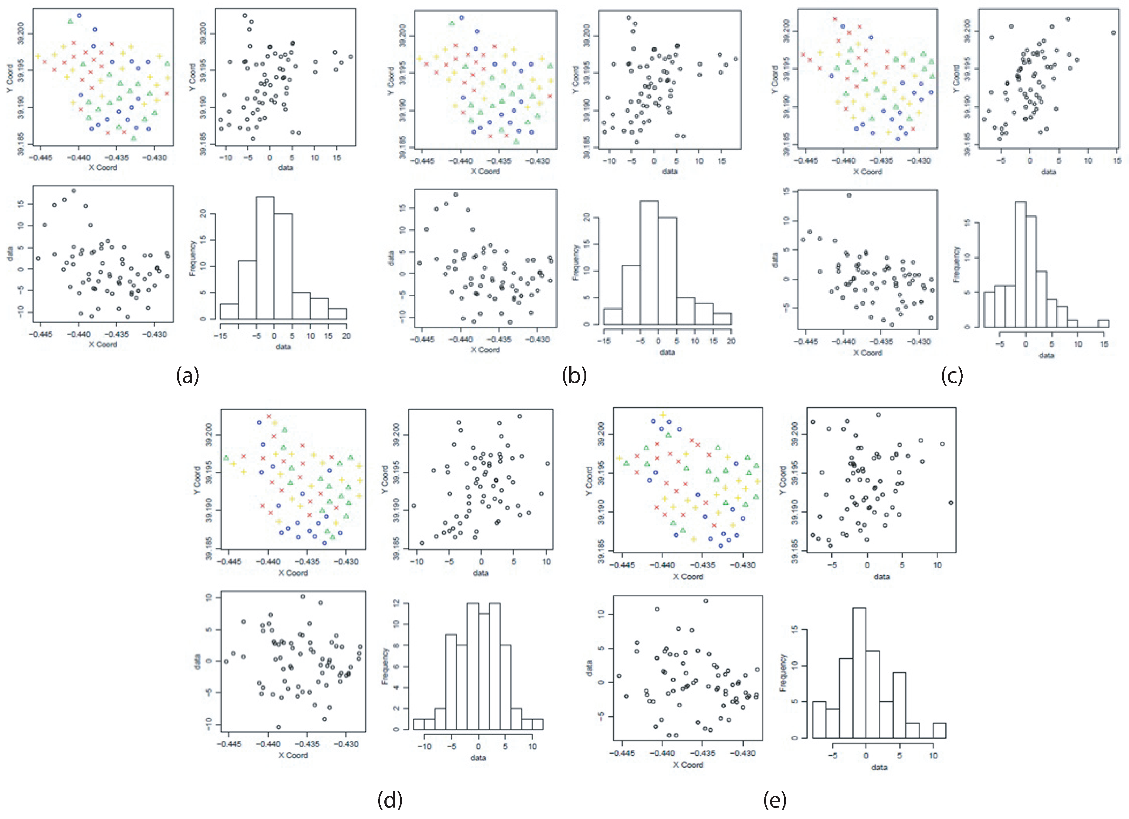
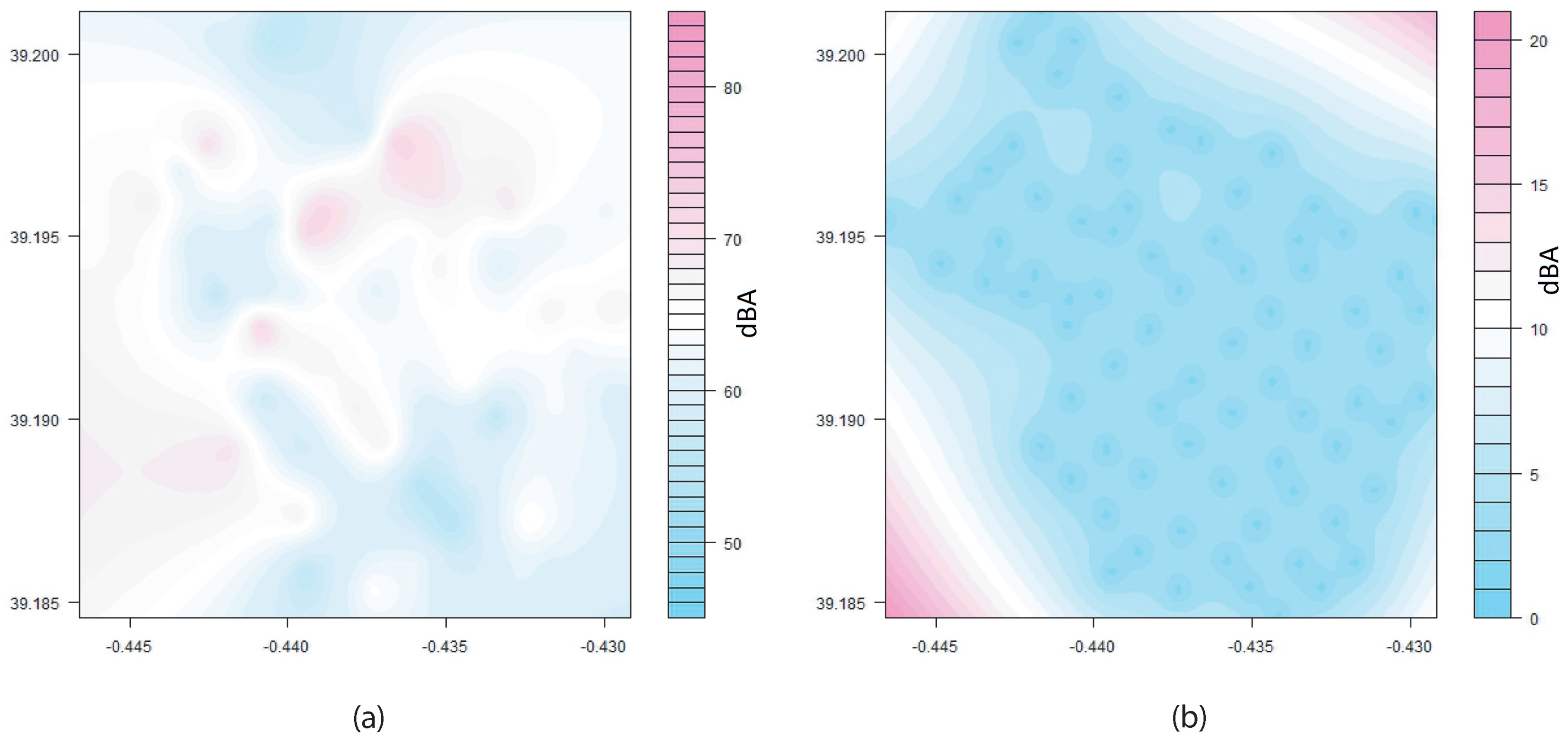
Table 4 gathers the tendency estimations of both parameters and their errors for the data in the five time periods. Once the tendency is adjusted, a first analysis of the spatial structure of the residuals has been conducted. The residuals have been represented graphically in the geographical coordinates (Figure 6) and a contrast test has been performed to check the spatial independence of the observations [30]. The nugget effect (see variogram part of Table 4) can be attributed to measurement errors or spatial sources of variation at smaller distances than the sampling interval (or both). Measurement errors occur due to the inherent error in measuring devices. Natural phenomena can vary spatially over a range of scales (i.e., micro or macro scales). Variation at micro scales smaller than the sampling distances will appear as part of the nugget effect. When looking at the model of a semivariogram, it is noticeable that, at a certain distance from the measurement points of the model, the error levels are higher but bounded (see Figure 7b). The distance where the model first flattens out is known as the range (in this case, the range is related to the arc seconds of the coordinates). The sill is the value where the semivariogram model attains the range (the value on the y-axis).

Table 4.
Summary of the spatial-temporal analysis of noise levels.
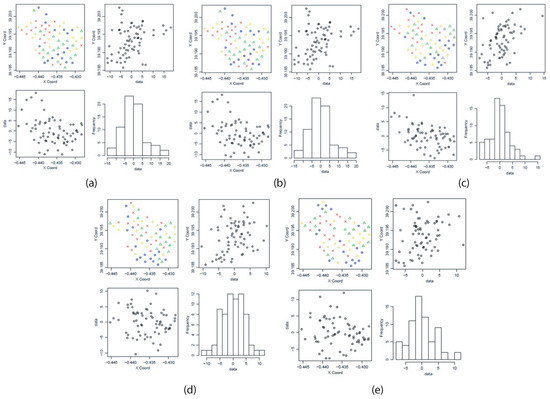
Figure 6.
Residuals for different time periods (upper left: spatial distribution of residuals grouped into four magnitude intervals, upper right: residuals according to latitude, lower left: residuals according to longitude, lower right: histogram of residuals). (a) period 1; (b) period 2; (c) period 3; (d) period 4; and (e) Period 5.

Figure 7.
(a) average estimated noise level; and (b) average prediction error.
From the P-values in the independence test shown in Table 3 and the graphics shown in Figure 6, we can say that the residuals are spatially correlated in all the time periods, except for the time period 5 (Figure 6e). The time periods 1 and 4 have a unique dependence in latitude, while periods 2 and 3 are correlated in both coordinates. This spatial correlation observed in Figure 6 is probably related to the orientation of most of the streets in the town. If the orientation of the streets is considered in the plan of the town, they are mostly oriented in the predominant direction North–South.
The adjustment of exponential isotropic variograms for the five data sets is done by using the Restricted Maximum Likelihood method (REML), which allows combining recursively the coefficients of the tendency , , and the components of the variogram. These values are shown in Table 4.
The goodness of the fitted model to each time period has been evaluated from the predictions of the noise level in the 10 locations of the validation set. The mean squared error (MSE) of these predictions has been obtained. Table 4 shows two values of the MSE. The first, MSE.lm, is calculated with the predictions obtained using the model fitted to the trend without making use of the residuals spatial modeling. The second, MSE.glm, is obtained from the predictions provided by the OK method.
An alternative way to measure the goodness of the fitting is based on cross-validation (CRV) over the modeling set itself, as suggested in [36]. The authors introduce three quantities to measure the goodness of model fitting: CRV1 contrasts with the unbiasedness of the prediction and its value must be equal to 0; CRV2 measures the accuracy of the standard deviation of the prediction error and its value is around 1; and finally CRV3 which measures the prediction error. The last row of Table 4 shows the values of these three parameters.
From the observation of Table 4, it appears that, from the point of view of the spatial prediction, modeling does not seem to have any advantage over the simple use of the trend. However, the goodness of fit is enhanced by spatial techniques, the values of the CRVx.glm clearly improve the CRVx.glm (these values are not shown in the table for this reason).
In order to cross-check the validity of the number of selected points, a Leave-One-Out- Cross-Validation algorithm in R (with the “Regularized Random Forest” method) has been used for the whole set of time averaged measurements. Table 5 shows the results of this test to select the nodes and generates a model to predict the % established in the first column (%test/%training). In this table, mtry stands for the number of randomly selected predictors, coefReg is the regularization value and coefImp is the importance coefficient. The RMSE is the minimum of the list of results obtained with this algorithm. According to this table, the selection of the validation set is enough for our network of measuring nodes. The test set has been checked against the model and the difference is in the range of the recommendation of the ISO 1996-2.

Table 5.
Summary of Leave-One-Out-Cross-Validation test using Regularized Random Forest (RRF) method.
Figure 8 shows a representation of the time evolution of the noise levels in Algemesí. This representation shows that the entrance to the city and its main roads (corresponding to Generalitat Av. and Ronda del Calvari in the left and upper part of the Figure) are the most noise polluted. This is due to the amount of vehicles passing through these main streets. In addition, in this area, the mean speed was reported to be higher than in other locations.
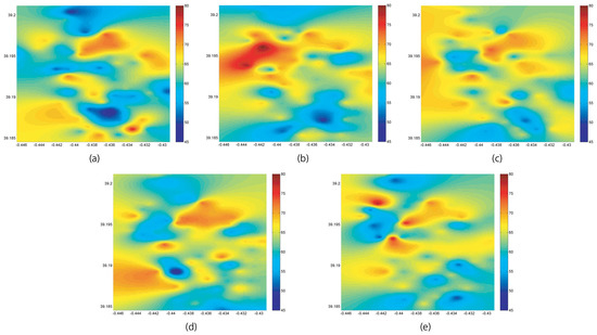
Figure 8.
Interpolated noise levels per time period: (a) 7–10 h; (b) 10–13 h; (c) 13–16 h; (d) 16–19 h and (e) 19–22 h.
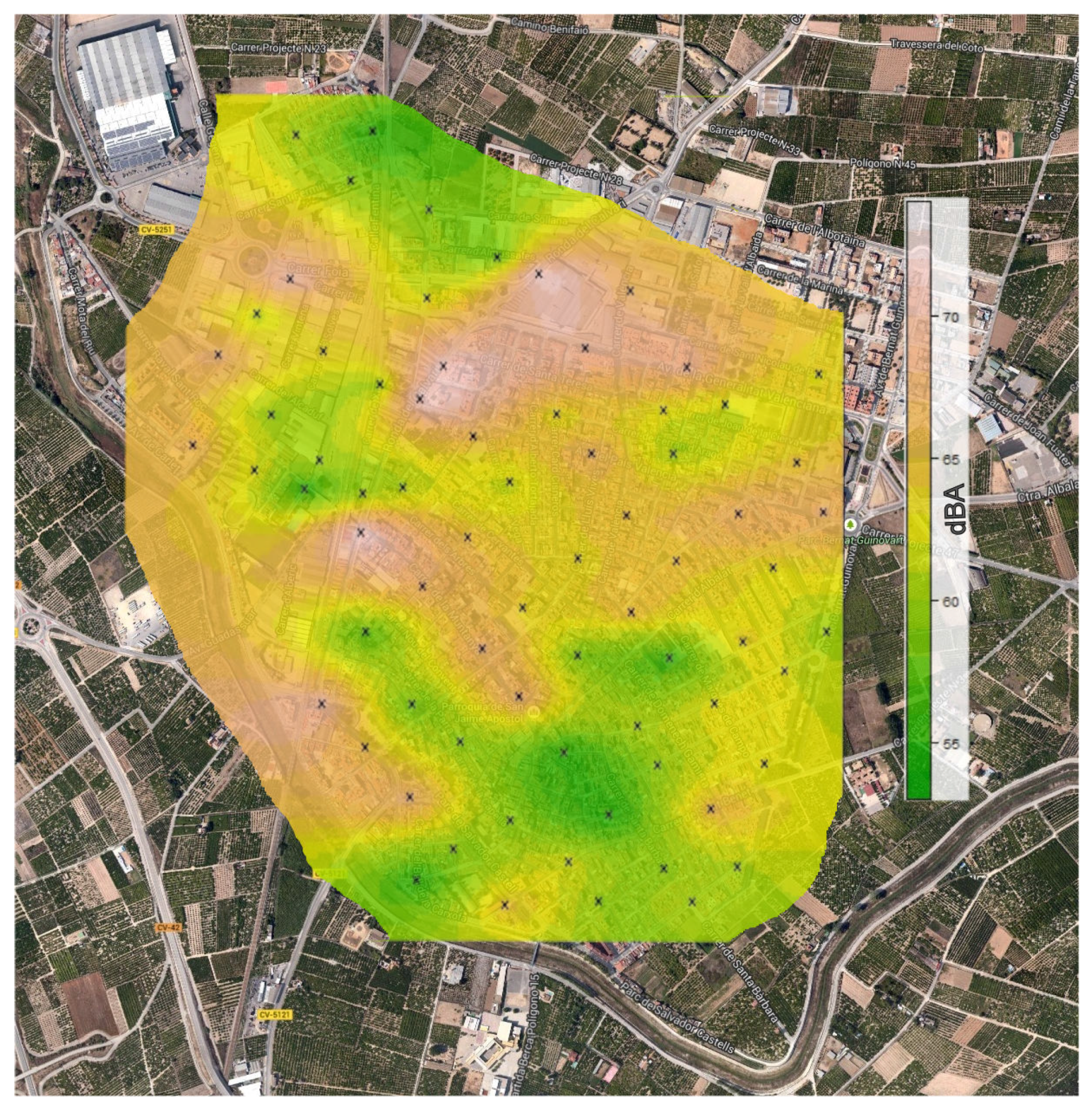
From the models obtained by using this analysis, we have been able to make predictions and their variances with OK. Using geoR library [37], Figure 9 shows a representation of the average noise levels in Algemesí on a 50 by 50 grid for the average value of the taking into account all the time periods. A representation of the noise levels on a plan of Algemesí (Valencia) can be observed together with the kriging of the time average values for each measuring point, so this kriging should be representative enough for all the time periods.

Figure 9.
Interpolated time-average noise levels on a map layer.
4. Conclusions
In this paper, a distributed noise measurement system based on Internet of Things (IoT) technology developed with Raspberry Pi nodes and a data collection system based in OpenCPU framework, which is related to the R statistical programming language, has been tested to measure the hourly sound pressure level evolution.
With this data, the application of a geostatistical method for interpolating spatial noise levels in a small-sized city in Valencia has been presented. The methodology makes the determination of the simultaneous spatial variation of noise levels in different time periods possible. From the results obtained, some notable conclusions can be extracted. One of them is that the kriging method has been proven as an efficient method to show noise level information in real-time. In addition, the residuals are spatially correlated in most time periods, except for time period 5. Perhaps, this fact is due to the spatial variation of the noise levels in the whole measuring grid in this period. For this reason, the last time period has been excluded in the model, due to the spatial non-correlation of the residuals in the period between 19 h and 22 h.
The goodness of the model in each time period has been checked from the predictions of the noise level in the 10 locations of the validation set (i.e., 13% of the nodes). The results have proven the validity of the spatial model in four time periods. This can be also checked within the cross validation results.
The methodology allows for representing these noise models, enabling the localization of critical areas in different time periods and the prediction of noise levels in different parts of the city. It also allows for showing that the noise levels are highly dependent on the spatial statistic model defined [38].
This method differs greatly from the issue of the subjective assessment of the noise annoyance, which poses quite a problem for those who are interested in developing and standardising units of measurement that convey the extent of the intensity of noise. It is also well-known that the decibel and the A-weighted system were developed precisely for this purpose, but they are far from being perfect [39]. At this point, it is worth mentioning that great efforts are being made for the soundscape description that is being standardised in ISO 12913 [40].
Further work on these issues is currently being done by increasing the number of measuring nodes in the WASN to measure urban noise, also previewed to collect full day measurements to compute parameters , and . This technology in combination with the explained methodology is a promising powerful tool for real-time distributed noise measurement and assessment.
Acknowledgments
Authors would like to thank the Spanish Ministry of Economy and Innovation for the funding, coming from the grant TEC2012-37945-C02-02 and the grant BIA2016-76957-C3-1-R.
Author Contributions
Jaume Segura Garcia, Juan Jose Pérez Solano, Santiago Felici Castell and Máximo Cobos Serrano conceived and designed the network and the experiments; Jaume Segura Garcia, Antonio Soriano Asensi and Enrique A. Navarro Camba performed the experiments; Francisco Montes Suay and Enrique A. Navarro Camba analyzed the data and made all the statical analysis; Santiago Felici Castell and Juan Jose Pérez Solano contributed with the WASN nodes; Jaume Segura Garcia wrote the paper.
Conflicts of Interest
The authors declare no conflict of interest. The funding sponsors had no role in the design of the study; in the collection, analyses, or interpretation of data; in the writing of the manuscript, and in the decision to publish the results.
Abbreviations
| ANOVA | Analysis of Variance |
| CRV | Cross-Validation |
| GIS | Geographic Information System |
| GNU/Linux | GNU’s Not Unix, Linux |
| GPU | Graphic Processing Unit |
| IoT | Internet of Things |
| MSE | Mean Squared Error |
| OK | Ordinary Kriging |
| REML | Restricted Maximum Likelihood method |
| RPi | Raspberry Pi |
| RRF | Regularized Random Forest |
| SoC | System on a Chip |
| TmI | Tmote Invent |
| WASN | Wireless Acoustic Sensor Networks |
| WSN | Wireless Sensor Networks |
References
- Santini, S.; Ostermaier, B.; Adelmann, R. On the Use of Sensor Nodes and Mobile Phones for the Assessment of Noise Pollution Levels in Urban Environments. In Proceedings of the 6th International Conference on Networked Sensing Systems (INSS 2009), Pittsburg, CA, USA, 17–19 June 2009.
- Renterghem, T.V.; Thomas, P.; Dominguez, F.; Dauwe, S.; Touhafi, A.; Dhoedt, B.; Botteldoren, D. On the ability of consumer electronics microphones for environmental noise monitoring. J. Environ. Monit. 2011, 13, 544–552. [Google Scholar] [CrossRef] [PubMed]
- Directive of the European Parliament. Directive 2002/49/EC of the European Parliament and of the Council of 25 June 2002 relating to the assessment and management of environmental noise. Off. J. Eur. Communities 2002, L189, 12–25. [Google Scholar]
- Santini, S.; Vitaletti, A. Wireless sensor networks for environmental noise monitoring. In Proceedings of the 6th GI/ITG KuVS Workshop Wireless Sensor Networks, Aachen, Germany, 16–17 July 2007; pp. 98–101.
- Santini, S.; Ostermaier, B.; Vitaletti, A. First experiences using wireless sensor networks for noise pollution monitoring. In Proceedings of the 3rd ACM Workshop Real-World Wireless Sensor Network (REALWSN), Glasgow, Scotland, UK, 1–4 April 2008; pp. 61–65.
- Polastre, J.; Szewczyk, R.; Culler, D. Telos: Enabling ultra-low power wireless research. In Proceedings of the 4th International Symposium on Information Processing in Sensor Networks (IPSN), Los Angeles, CA, USA, 24–27 April 2005; pp. 364–369.
- Hakala, I.; Kivelä, I.; Ihalainen, J.; Luomala, J.; Gao, C. Design of low-cost noise measurement sensor network: Sensor function design. In Proceedings of the IEEE 1st International Conference on Sensor Device Technologies and Applications, Venice, Italy, 18–25 July 2010; pp. 172–179.
- Kivelä, I.; Gao, C.; Luomala, J.; Hakala, I. Design of noise measurement sensor network: Networking and communication part. In Proceedings of the 5th International Conference on Sensor Technologies and Applications, Côte d’Azur, France, 21–27 August 2011; pp. 280–287.
- Maisonneuve, N.; Stevens, M.; Niessen, M.E.; Hanappe, P.; Steels, L. Citizen noise pollution monitoring. In Proceedings of the 10th Annual International Conference on Digital Government Research: Social Networks: Making Connections between Citizens, Data and Government, Digital Government Society of North America, Puebla, Mexico, 17–21 May 2009; pp. 96–103.
- Maisonneuve, N.; Stevens, M.; Niessen, M.E.; Steels, L. Noise-Tube: Measuring and mapping noise pollution with mobile phones. In Information Technologies in Environmental Engineering (Environmental Science and Engineering); Athanasiadis, I., Rizzoli, A.E., Mitkas, P.A., Gómez, J.M., Eds.; Springer: Verlag/Berlin, Germany, 2009; pp. 215–228. [Google Scholar]
- Di-Francesco, M.; Das, S.K.; Anastasi, G. Data collection in wireless sensor networks with mobile elements: A survey. ACM Trans. Sens. Netw. 2011, 8. [Google Scholar] [CrossRef]
- Cressie, N. Statistics for Spatial Data; John Wiley: New York, NY, USA, 1993. [Google Scholar]
- Baume, O.; Gauvreau, B.; Bérengier, M.; Junker, F.; Wackernagel, H.; Chilès, J. Geostatistical modeling of sound propagation: Principles and a field application experiment. J. Acoust. Soc. Am. 2009, 126, 2894–2904. [Google Scholar] [CrossRef] [PubMed]
- Harman, B.; Koseoglu, H.; Yigit, C.O. Performance evaluation of IDW, Kriging and multiquadric interpolation methods in producing noise mapping: A case study at the city of Isparta, Turkey. Appl. Acoust. 2016, 112, 147–157. [Google Scholar] [CrossRef]
- Broadcom Corp., Ltd. (UK). BCM2835 ARM Peripherals. Available online: https://www.raspberrypi.org/wp-content/uploads/2012/02/BCM2835-ARM-Peripherals.pdf (accessed on 11 November 2016).
- ARM Ltd. (UK). ARM1176JZF-S: Technical Reference Manual. Available online: http://infocenter.arm.com/help/topic/com.arm.doc.ddi0301h/DDI0301H_arm1176jzfs_r0p7_trm.pdf (accessed on 11 November 2016).
- Logilink, 2direct GmbH (Germany). Logilink USB to Audio Adapter Mod. UA0053 specifications. Available online: http://www.logilink.eu/media/datasheets/UA0053.pdf (accessed on 11 November 2016).
- CUI Inc. Electret condenser microphone Mod. CMA-4544PF-W. Available online: http://www.cui.com/product/resource/cma-4544pf-w.pdf (accessed on 11 November 2016).
- TP-LINK Technologies Co., Ltd. TP-Link TL-WN725N specifications. Available online: http://www.tp-link.com/en/products/details/TL-WN725N.html (accessed on 11 November 2016).
- Kodak Co. (Rochester, NY, USA). Kodak KD LR20 battery specifications. Available online: http://www.kodak.com/eknec/documents/fe/0900688a8019d7fe/KD.pdf (accessed on 11 November 2016).
- Upton, E.; Halfacree, G. Raspberry Pi User Guide, 3rd ed.; John Wiley and Sons Ltd.: Chichester, UK, 2014. [Google Scholar]
- Chroboczek, J. The Babel Routing Protocol, RFC 6126, Quagga Routing Software Suite, GPL Licensed, 2011. Available online: http://www.quagga.net (accessed on 3 October 2016).
- Patawari, A. Getting Started with OwnCloud; Packt Publishing Ltd.: Birmingham, UK, 2013. [Google Scholar]
- Brocolini, L.; Lavandier, C.; Quoy, M.; Ribeiro, C. Measurements of acoustic environments for urban soundscapes: Choice of homogeneous periods, optimization of durations, and selection of indicators. J. Acoust. Soc. Am. 2013, 134, 813–821. [Google Scholar] [CrossRef] [PubMed]
- Geraghty, D.; O’Mahony, M. Investigating the temporal variability of noise in an urban environment. Int. J. Sustain. Built Environ. 2016, 5, 34–45. [Google Scholar] [CrossRef]
- Ooms, J. The OpenCPU system: Towards a universal interface for scientific computing through separation of concerns. arXiv, 2014; arXiv:1406.4806. [Google Scholar]
- CESVA SL (Spain). SC310 - Sound Level Meter and Spectral Analyser. Available online: https://download.cesva.com/datasheets/sc310_eng.pdf (accessed on 3 November 2016).
- Garcia, A. Environmental Urban Noise; WIT Press: Southampton, UK, 2001. [Google Scholar]
- RPi Camera. Raspberry Pi Camera v2 specifications. Available online: http://www.farnell.com/datasheets/2056179.pdf?_ga=1.152577328.880870297.1479740269 (accessed on 11 November 2016).
- Diblasi, A.; Bowman, A.W. On the use of the variogram in checking for independence in spatial data. Biometrics 2001, 57, 211–218. [Google Scholar] [CrossRef] [PubMed]
- R webpage. Available online: http://www.r-project.org/ (accessed on 3 August 2016).
- Quinones-Bolanos, E.E.; Bustillo-Lecompte, C.F.; Mehrvar, M. A traffic noise model for road intersections in the city of Cartagena de Indias, Colombia. Transp. Res. Part D Transp. Environ. 2016, 47, 149–161. [Google Scholar] [CrossRef]
- Halim, H.; Abdullah, R. Equivalent noise level response to number of vehicles: A comparison between a high traffic flow and low traffic flow highway in Klang Valley, Malaysia. Front. Environ. Sci. 2014, 2. [Google Scholar] [CrossRef]
- Segura, J.; Navarro, E. Estudio de la Contaminación Acústica en el Municipio de Algemesí “Study of the Acoustic Pollution in the Municipality of Algemesí”; Universitat de València: Burjassot, Spain, February 2011. [Google Scholar]
- García-Rodríguez, A. Estudio del Ruido Ambiental en la Comunidad Valenciana “Study of the Environmental Noise in the Valencian Community”; Generalitat Valenciana: València, Spain, 1994. [Google Scholar]
- Huang, H.C.; Cressie, N. Spatio-temporal prediction of snow water equivalent using the Kalman filter. Comput. Stat. Data Anal. 1996, 22, 159–175. [Google Scholar] [CrossRef]
- Ribeiro, P.J.; Diggle, P.J. geoR: A package for geostatistical analysis. R-News 2001, 1, 15–18. [Google Scholar]
- Ryu, H.; Park, I.K.; Chun, B.S.; Chang, S.I. Spatial statistical analysis of the effects of urban form indicators on road-traffic noise exposure of a city in South Korea. Appl. Acoust. 2017, 115, 93–100. [Google Scholar] [CrossRef]
- Murphy, E.; King, E. Environmental Noise Pollution: Noise Mapping, Public Health, and Policy; Elsevier Inc.: San Diego, CA, USA, 2014. [Google Scholar]
- ISO 12913-1:2014 Acoustics—Soundscape—Part 1: Definition and Conceptual Framework. Available online: http://www.iso.org/iso/catalogue_detail.htm?csnumber=52161 (accessed on 25 October 2016).
© 2016 by the authors; licensee MDPI, Basel, Switzerland. This article is an open access article distributed under the terms and conditions of the Creative Commons Attribution (CC-BY) license (http://creativecommons.org/licenses/by/4.0/).

