Abstract
Parallel analyses about the dynamic responses of a large-scale water conveyance tunnel under seismic excitation are presented in this paper. A full three-dimensional numerical model considering the water-tunnel-soil coupling is established and adopted to investigate the tunnel’s dynamic responses. The movement and sloshing of the internal water are simulated using the multi-material Arbitrary Lagrangian Eulerian (ALE) method. Nonlinear fluid–structure interaction (FSI) between tunnel and inner water is treated by using the penalty method. Nonlinear soil-structure interaction (SSI) between soil and tunnel is dealt with by using the surface to surface contact algorithm. To overcome computing power limitations and to deal with such a large-scale calculation, a parallel algorithm based on the modified recursive coordinate bisection (MRCB) considering the balance of SSI and FSI loads is proposed and used. The whole simulation is accomplished on Dawning 5000 A using the proposed MRCB based parallel algorithm optimized to run on supercomputers. The simulation model and the proposed approaches are validated by comparison with the added mass method. Dynamic responses of the tunnel are analyzed and the parallelism is discussed. Besides, factors affecting the dynamic responses are investigated. Better speedup and parallel efficiency show the scalability of the parallel method and the analysis results can be used to aid in the design of water conveyance tunnels.
1. Introduction
The dynamic responses of a buried tunnel in general, and its seismic responses, in particular, are of much interest [1,2,3]. The water conveyance tunnel, as one kind of urban underground tunnel, guarantees domestic water for residents in metropolises, and is considered as the lifeline to a city. Actual seismic events have shown that tunnels are easily damaged during earthquakes [4,5]. Thus, the seismic analysis and anti-seismic design of the tunnels are important and necessary. The traditional analytical method and two dimensional or simplified three dimensional analysis methods may create some inaccuracies, such as the overestimation or underestimation of tunnel deformations [6]. Due to the fact that the soil-structure interaction (SSI) is complicated and the underground structures may induce wave diffraction [7], it may need the help of the finite element method (FEM) to get accurate results especially under realistic conditions [8,9,10].
Although the water conveyance tunnel characterized by the inner water is different from normal immersed tunnels, general analysis approaches are still suitable. The study of a water conveyance tunnel under seismic loadings involves interaction between inner water and tunnel structures. The interaction between fluid and structure of the liquid storage vessels under seismic loading was first studied by Westergaard [11]. Afterwards, lots of pioneering work was performed by Housner [12], and the added mass method provided by him has been widely used in relation to structure design codes and standards. On the basis of the previous work, other scholars have studied and developed the relevant algorithms [13]. All the above-mentioned studies mainly focus on the responses of the vertical cylindrical or rectangular tanks and the analogous morphing structures. On the contrary, studies on seismic responses of the horizontal cylindrical liquid storage vessels to which the water conveyance tunnel with water–structure interaction belongs are limited. The earliest research of this kind of problems can be found in the literature [14]. After that researchers have made further studies [15,16]. With the development of high-performance computing, full scale numerical simulations considering fluid–structure interaction (FSI) emerge constantly, among which the Arbitrary Lagrangian Eulerian (ALE) based fluid structure coupling algorithm has been used widely. Cao, et al. [17] have analyzed the dynamic responses of a flexible container subjected to wind actions using the ALE based fluid–structure interaction method. Zhao, et al. [18] have used the ALE to simulate the fluid–structure interaction of the AP1000 water tank subjected to earthquakes and obtained the optimal height of water to reduce seismic responses. It is thus clear that the ALE based fluid–structure interaction algorithm can be used to deal with the coupling of liquid and its corresponding storage vessel [19,20,21]. Thus, the ALE based fluid–structure interaction approach is adopted in this study for analyses of the water conveyance tunnel subjected to earthquakes.
To solve the efficiency problem arising from a large-scale finite element calculation, the aids from high-performance computers and parallel algorithms are necessary. Though a number of ideas for parallelized finite element computational methods have been developed [22], the further study for one such scale model with lots of detections and computations for contact (including SSI) and FSI is still needed to obtain more even load distribution and higher parallel efficiency. In this paper, a modified domain decomposition technique derived from the recursive coordinate bisection (RCB) method, which is named the modified RCB (MRCB), is proposed. This method splits the model based on its topological distribution of the computation loads as well as its geometric shape. Not only is the number of nodes and elements in each partition approximately equal, but also the extra coupling loads including contact and FSI are almost balanced. Therefore, the total amount of computation for every processor core is nearly equivalent, and a higher parallel efficiency can be obtained. In this study, the proposed domain decomposition (MRCB) based parallel computing method is used for analyses of the water conveyance tunnel subjected to earthquakes.
The reminder of the paper is divided as follows. The methodologies for parallel numerical computation including ALE based fluid–structure interaction algorithm, the proposed domain decomposition (MRCB) based parallel solving algorithm and other related key techniques are introduced in Section 2. Section 3 contains the detailed descriptions for the numerical model of the water conveyance tunnel. In Section 4, the model and the proposed approaches are verified through comparison with the added mass method, and then the seismic behaviors of the specific tunnel and the performance of the parallel method are addressed and discussed; furthermore, factors that affect the dynamic responses of the tunnel are analyzed. Finally, Section 5 gives some conclusions about this study.
2. Methodologies for Parallel Numerical Computation
2.1. Arbitrary Lagrangian-Eulerian Based Fluid–Structure Interaction
The water conveyance tunnel is different from the normal shield tunnels because of the water inside the tunnel. The interaction between water and tunnel affects the seismic responses of the tunnel [23]. The ALE method has been demonstrated as an effective way to tackle the FSI problems [17,18,24,25]. Therefore, in this study the ALE method is adopted to perform the FSI during seismic analysis of the water conveyance tunnel.
The mass and momentum governing equations [17] of the ALE method are expressed as Equations (1) and (2).
where , , , , and signify the ALE coordinates, density, velocity of material (fluid), body force, velocity of convection and stress tensor, respectively.
With regard to the tunnel structure, its deformation can be given with a constitutive equation as:
where , , and signify the Lagrangian coordinate, the displacement, Lagrangian structure density and the body force, respectively.
On the FSI interface, the geometric compatibility and mechanical equilibrium conditions (Equations (4) and (5)) [17] should be satisfied, which cause the coupling of Equations (1)–(3).
where , are the interactive force of fluid and structure arising at the FSI interface, respectively.
The interaction force is calculated by using the penalty function method. The penalty function based FSI system is shown in Figure 1, where P, R and D represents the penetration, the penalty rigidity and the damping coefficient, respectively. The basic idea of the penalty function method is to assure that there is no penetration at the coupling interface by introducing the coupling force between fluid and structure. During the simulation, if the penetration appears, a coupling force will be introduced, and the high frequency is damped out with the purpose of restraining numerical oscillation.
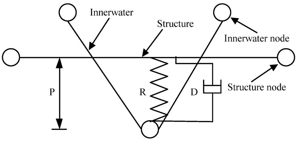
Figure 1.
Fluid–structure interaction (FSI) with viscous damper system. P, R and D represents the penetration, the penalty rigidity and the damping coefficient, respectively.
Figure 1.
Fluid–structure interaction (FSI) with viscous damper system. P, R and D represents the penetration, the penalty rigidity and the damping coefficient, respectively.

2.2. Nonlinear Contact Algorithm
The soil-tunnel contact is simulated in this study with automatic contact conditions. Therefore, the potentially realistic forces at the contact zone can be simulated [26]. The penalty function method is adopted as the solution algorithm for contact [8]. In the penalty algorithm, contact conditions are imposed by penalizing the inter-penetration among contacting surfaces. When there is no penetration, nothing will be done; when a penetration is detected, a coupling force will be introduced between tunnel and soil.
The frictional behavior between full-slippling and no-slippling at the contact interface exits [27]. Aiming at modeling the contact conditions for the SSI in this tunnel project properly, the standard Coulomb friction law is employed.
2.3. Explicit Finite Element Time Integration
The mathematical representation of the specific nonlinear coupling system under seismic excitation can be described as:
where , and signify the generalized acceleration, velocity, and displacement vectors, respectively; , and mean the matrices of stiffness, damping and mass separately; means the vector of internal resisting forces, and represents the vector of the external forces.
The explicit central difference approach has been used to deal with the system equations. Assuming that and are variable time intervals, the variants updating at time are given by:
The explicit central difference algorithm is only stable under the Courant conditions [28]. This should be taken into consideration during the simulation.
2.4. Domain Decomposition Technique
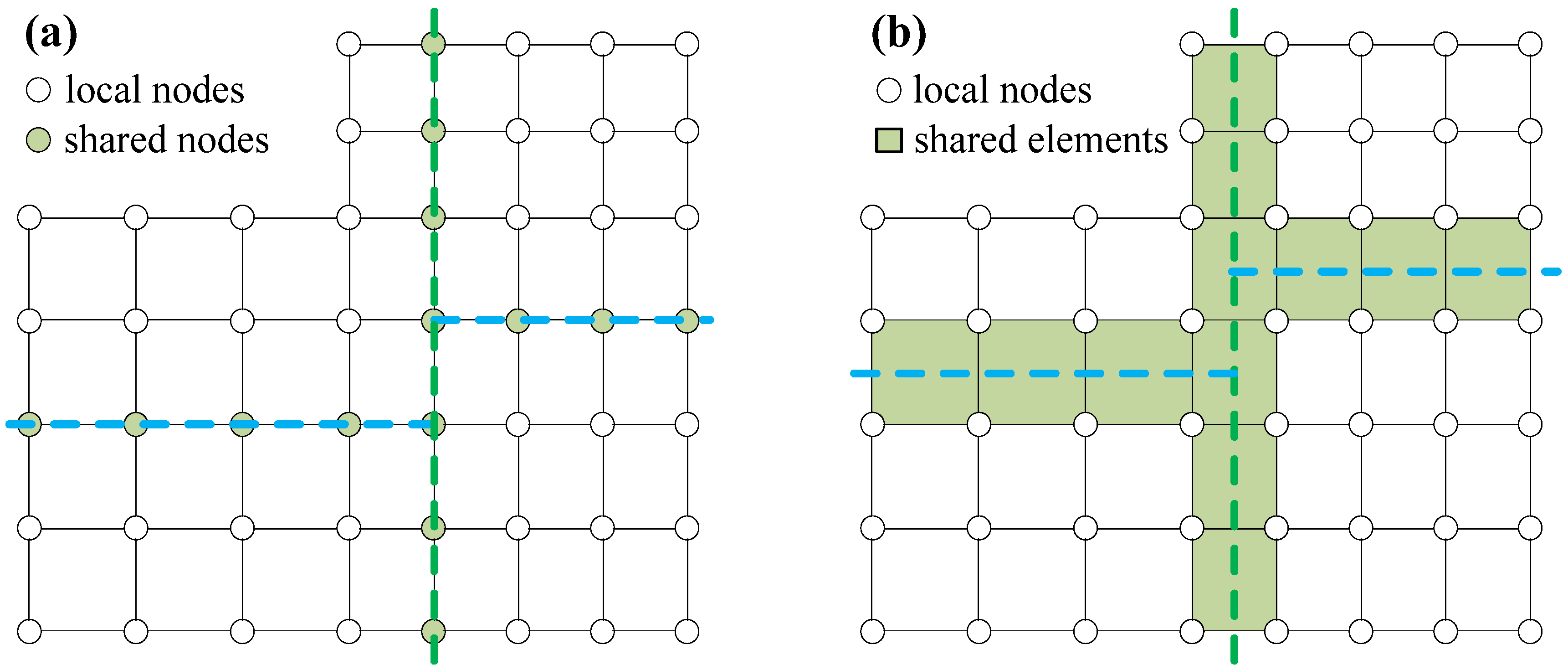
The domain decomposition method (DDM) is used in this study. Overlapping and non-overlapping methods are the two main classes of DDMs, and the non-overlapping method is more suitable for parallel computing architectures [29]. There exist two main kinds of non-overlapping DDMs for the finite element mesh, namely, the node-cut concept and the element-cut concept (see Figure 2). In the node-cut approach, the individual mesh elements are assigned to unique partitions (Figure 2a), and the shared nodes are duplicated to each partition who owns the nodes (filled circles in Figure 2a). On the contrary, the element-cut approach is based on a unique assignment of mesh nodes to unique partitions (Figure 2b), and the shared elements are duplicated to each partition to which their nodes belong (filled squares in Figure 2b). The communication among cores is through shared nodes or elements, respectively. Because the duplication effort is very little by sharing nodes among cores and the element-cut approach is generally less efficient, the node-cut approach has been used in the paper.
The parallelization of LS-DYNA MPP (massive and parallel processors) version is based on the domain decomposition technique, and currently the RCB (Recursive Coordinate Bisection) is the default algorithm. RCB can decompose a model rapidly and effectively. It can easily be executed at run-time without significant costs and get a good balance of computational loads [30]. However, RCB also has some drawbacks. For instance, the disconnected domains may be created during the partition for models with complex geometric shapes. Furthermore, the RCB algorithm is only based on the geometric information of the model, and the load distributions and contact positions are not considered. Thus, the partition quality of the large-scale realistic simulation model is not so good. Therefore, for large-scale realistic models like the seismic analysis model of water conveyance tunnel, the original RCB is not the best DDM because of the need for extensive contact and FSI computation. The RCB method should be optimized for the specific analysis model to get better parallel efficiency.

Figure 2.
Non-overlapping domain decomposition: (a) node-cut approach; (b) element-cut approach. The green and blue dotted lines mean different split locations.
Figure 2.
Non-overlapping domain decomposition: (a) node-cut approach; (b) element-cut approach. The green and blue dotted lines mean different split locations.
2.5. Modified Domain Decomposition Method (DDM) Considering Contact and Fluid–Structure Interaction (FSI) Load Balance
Taking the structure characteristics of the large-scale water conveyance tunnel and the computation features of the seismic analysis into account, one modified DDM, which is derived from the basic principles of RCB and named as the MRCB (modified RCB), has been proposed. The MRCB is optimized for the supercomputer Dawning 5000A (Sugon, TianJin, China) and used for the seismic research of the specific tunnel. The MRCB is subject to the following rules to keep the balance of the total loads in each subdomain: firstly, the coupling loads including FSI and contact can be almost evenly distributed to each subdomain; secondly, the total numbers of nodes and elements can be balanced in every subdomain; thirdly, the amount of communication among adjacent subdomains can be minimized; lastly, the convergence rate in each subdomain is increased and nearly equivalent. The novel point of this parallelization is the balance of coupling loads in each subdomain, rather than just the equivalence of nodes and elements. Thus, the total computation loads in each subdomain for each processor core is almost equal and the parallel efficiency is improved.
The basic idea of MRCB contains the following steps: firstly, a combined coordinate transformation is applied to the model according to its characteristics; then the domain decomposition approach is used to deal with the deformed model, and the model is divided into the required number of subdomains; finally, the original model is split by mapping the partitioned subdomains back. There exist a number of functions for coordinate transformation in LS-DYNA software (LSTC, Livermore, CA, USA), which provide aids to realize the MRCB. Considering the structure characteristics of the water conveyance tunnel project and its distribution features of CPU-intensive calculation, different portions of the model are decomposed by using different transformations to fulfill the abovementioned rules for the balanced domain decomposition. The solving procedure of the MRCB based parallel explicit algorithm is shown in Figure 3.
The basic idea of MRCB contains the following steps: firstly, a combined coordinate transformation is applied to the model according to its characteristics; then the domain decomposition approach is used to deal with the deformed model, and the model is divided into the required number of subdomains; finally, the original model is split by mapping the partitioned subdomains back. There exist a number of functions for coordinate transformation in LS-DYNA software (LSTC, Livermore, CA, USA), which provide aids to realize the MRCB. Considering the structure characteristics of the water conveyance tunnel project and its distribution features of CPU-intensive calculation, different portions of the model are decomposed by using different transformations to fulfill the abovementioned rules for the balanced domain decomposition. The solving procedure of the MRCB based parallel explicit algorithm is shown in Figure 3.
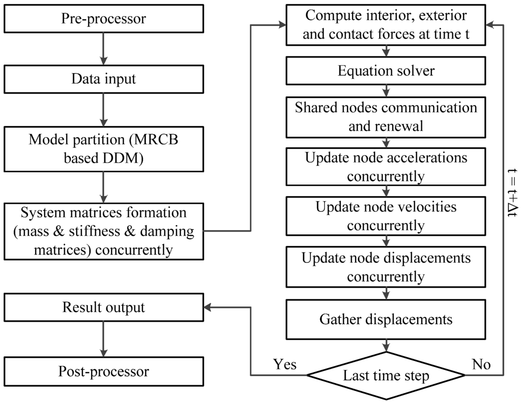
Figure 3.
Flow chart of the MRCB based parallel solving procedure. MRCB: modified recursive coordinate bisection; DDM: domain decomposition method.
Figure 3.
Flow chart of the MRCB based parallel solving procedure. MRCB: modified recursive coordinate bisection; DDM: domain decomposition method.

3. Model Description for Water Conveyance Tunnel
Dynamic responses of the newly built large-scale Qingcaosha water conveyance tunnel (QWCT) under seismic excitation are examined closely. The details of the simulation model and the computing environment are presented in the following subsections.
3.1. Tunnel Project
QWCT is a double-line tunnel with a length of 14 km which includes the Western tunnel and the Eastern tunnel (Figure 4). QWCT is divided into three parts by work shafts, including the island (Changxing island) part, the cross-rive (Yangtze river) part and the land (Pudong district) part. Different parts of the QWCT are connected through the work shafts, and there are five work shafts, as shown in Figure 4, which are also considered in this study. QWCT is composed of about 10,000 tunnel rings. Figure 5 shows one typical cross-section. QWCT conveys portable water for approximately 11 million people and accounts for more than half of the total raw water supply in Shanghai. Its seismic safety is directly related to the drinking water security of this metropolis and its aseismic performance needs to be properly examined.
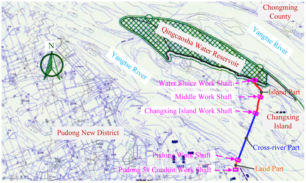
Figure 4.
Location of the Qingcaosha water conveyance tunnel.
Figure 4.
Location of the Qingcaosha water conveyance tunnel.
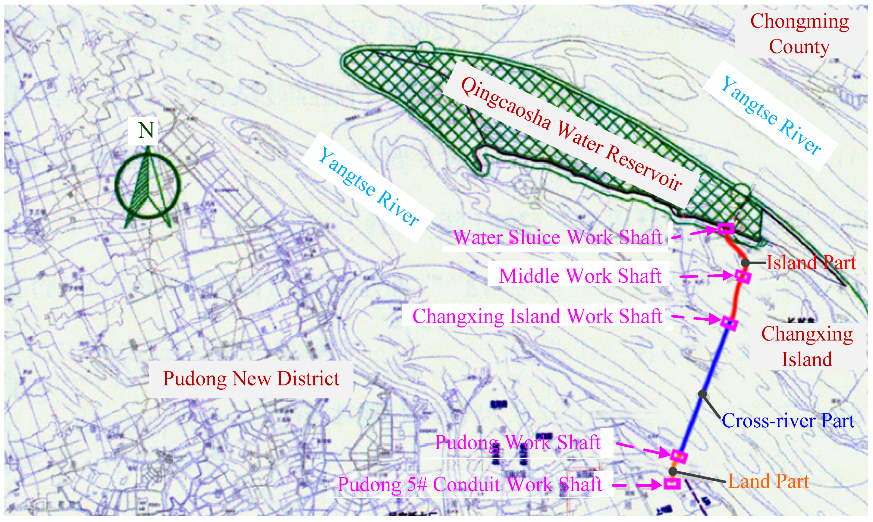
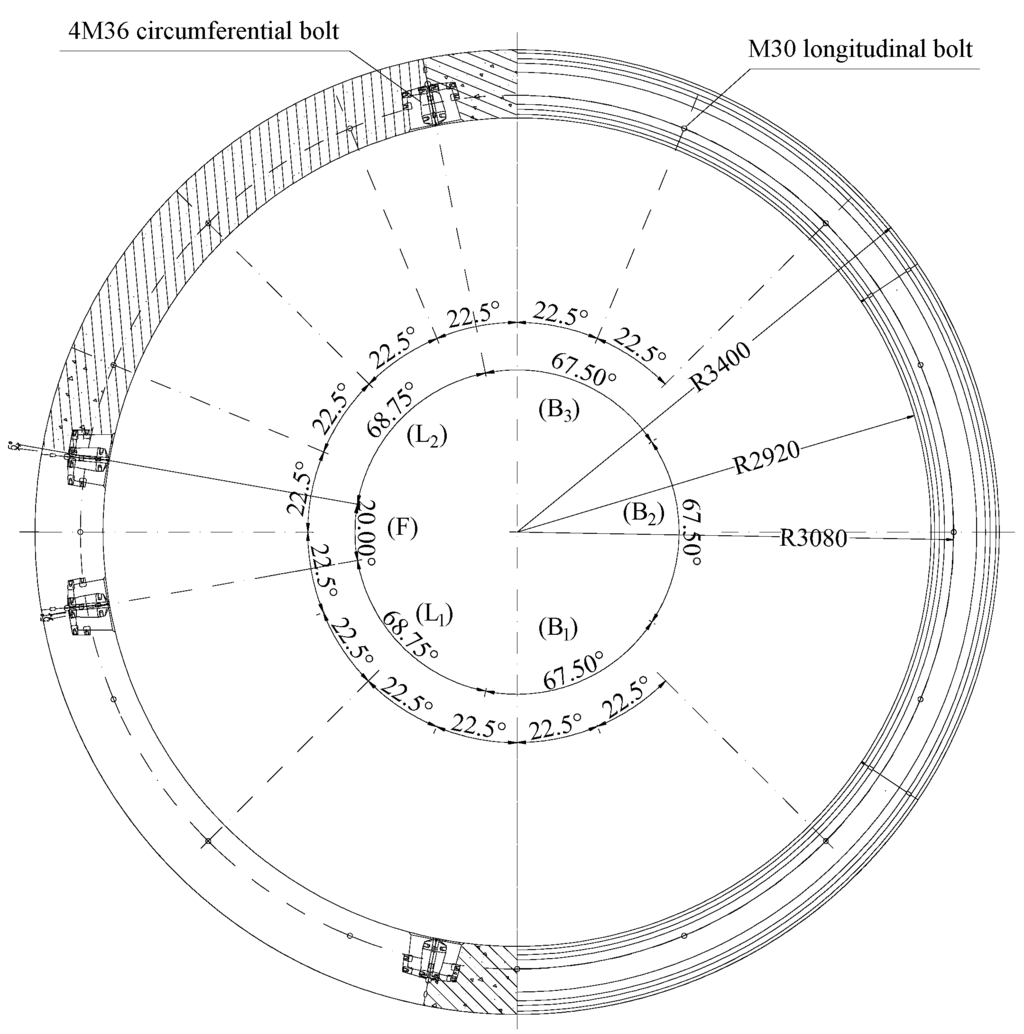
Figure 5.
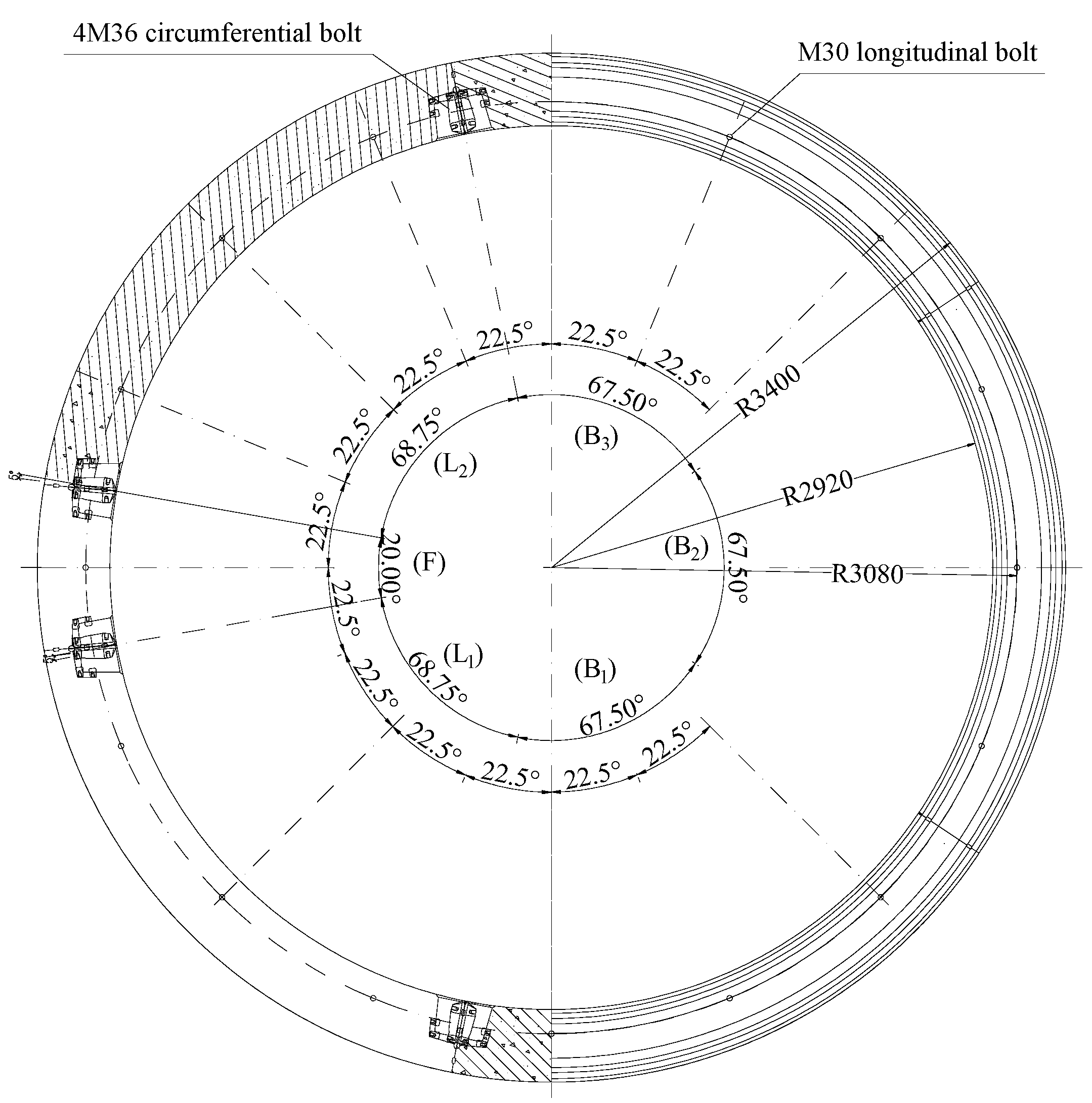
Typical cross-section of the tunnel (cross-river part).
Figure 5.
Typical cross-section of the tunnel (cross-river part).
3.2. Finite Element Model Overview
A full scale, three-dimensional finite element (FE) model of the QWCT tunnel has been constructed according to the geologic circumstance and design materials. The full scale FE model includes soil, tunnel, inner water, work shafts and deformation joints between tunnel and work shafts. The final three-dimensional size of the full scale FE model, which is composed of 1,668,760 elements and 1,913,524 nodes, is 13280 m × 5150 m × 300 m. Figure 6 and Figure 7 show the three-dimensional view of the established full scale FE model, and some more detailed depictions of the FE model are given in Figure 8. As shown in Figure 7, twenty-four typical cross-sections including IS1–IS9 in the island part, RS1–RS10 in the cross-river part and LS1–LS5 in the land part are chosen as the concerned locations.

Figure 6.
The whole finite element (FE) model of the tunnel-soil-water coupling system.
Figure 6.
The whole finite element (FE) model of the tunnel-soil-water coupling system.
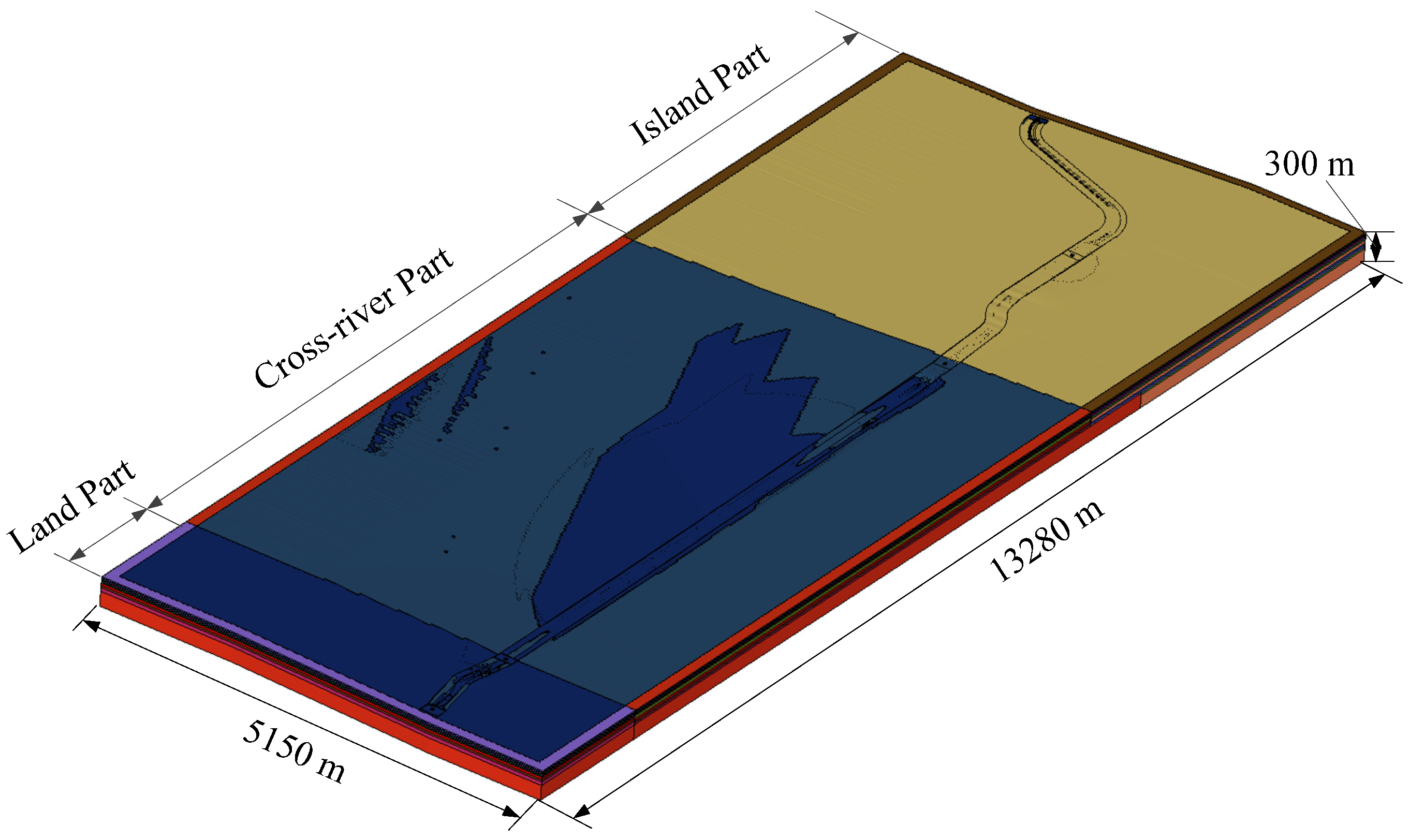
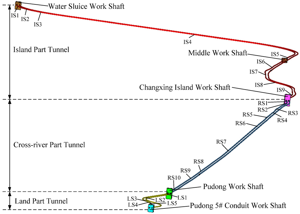
Figure 7.
The whole tunnel FE model and positions of the control sections. IS1–IS9, RS1–RS10 and LS1–LS5 depict the chosen control sections in the island, cross-river and land part, respectively.
Figure 7.
The whole tunnel FE model and positions of the control sections. IS1–IS9, RS1–RS10 and LS1–LS5 depict the chosen control sections in the island, cross-river and land part, respectively.

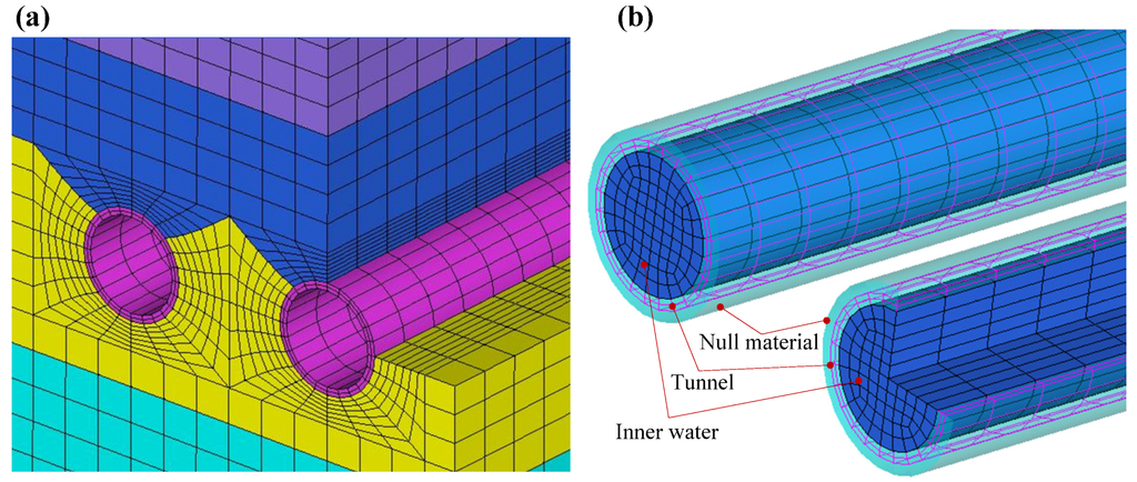
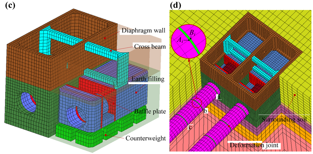
Figure 8.
Details of FE model: (a) tunnel and soil; (b) tunnel, inner water and null material; (c) typical work shaft; (d) work shaft and surrounding soil. a, b and c mean the first, second and third deformation joint, respectively; Ai and Bi denote the ith displacement at the left and right side of the deformation joint, respectively.


The tunnel is discretized with thick shell elements, the local coordinates of which are determined by the nodes of elements. The tunnel is treated as a homogeneous model, which is considered as an alternative [31] to get the whole responses of the tunnel and determine the dangerous cross-sections while maintaining a moderate system equation for computation. The mesh dimension is determined through a series of mesh sensitivity tests which also assure the accuracy of the results. The work shafts and their details are meshed with eight node hexahedron elements (excluding the pile foundation discretized with beam elements). The inner water is discretized with eight node hexahedron elements with ALE description. The deformation joints are also discretized with thick shell elements. The surrounding soil is established based on the geological data. The soil strata are divided into 10 layers with the elevation of −300 m which is the typical depth of bedrock in Shanghai. The soil model is meshed with eight node hexahedron elements. The whole model is discretized with fine meshes at the core area around the tunnel and coarse meshes at the other areas, and the fine and coarse meshes are coupled by node equivalence. This kind of discretization is considered as a time-saving method for large-scale numerical computation. The element sizes are determined according to the primary frequency of the input seismic wave to reduce the errors caused by model discretization. In this study, six elements per wavelength are adopted. The total number of elements in this study is similar to that of elements used in the previous seismic analysis for the underground tunnel [8].
3.3. Material Nonlinearity and Constitutive Model
The concrete model of the tunnel is assumed as the linear elastic material. Its mass density is 2500 kg/m3. Its elastic modulus is 35.5 GPa and its Poisson ratio is 0.2. The widely used rubber model of Mooney-Rivlin [25,32] is adopted for describing the deformation joints. The law of Mooney-Rivlin for the incompressible rubber is based on a strain energy function, which can be described as:
in which the material parameters derived from the uniaxial test data are represented by and ; the Cauchy-Green tensor invariants are described by , and , respectively; the Poisson ratio is represented by . The parameters of this material used in this study include mass density of 1300 kg/m3, a Poisson ratio of 0.4999, constant of 7.0 × 10⁵ Pa, and constant of 3.5 × 10⁵ Pa.
Because of the slight compressibility of the Newtonian fluid (inner water) used in this study, the viscous stress caused by volumetric change is nearly zero. So, the constitutive equation is given by:
where is pressure; is Kronecker-δ; signifies the deviatoric stress tensor. On the right side of Equation 13, the first item is defined with EOS (equation of state) in simulation; the second item is the deviatoric stress and is obtained through the material constitutive model.
The null material model is used to compute the deviatoric stress of the inner water. The EOS of inner water can be described by the Gruneisen equation with appropriately chosen parameters. The Gruneisen equation can be given as:
in which , and represent the slope factors for the curve of ; signifies the intercept for the curve of ; , , and represents Gruneisen gamma, kinematic viscosity, initial internal energy and a volume correction of , respectively. In this simulation, the variable parameters and are set as 1400 m/s and 8.684 × 10⁻⁴, respectively; the constant parameters , , and are 0.35, 0, 1.192, −0.92 and 0, respectively.
The soil is modeled with a Biot hysteretic material which is developed to represent the viscoelastic behavior of soils subjected to cyclic load, for example, in the SSI analysis under seismic excitation [33]. The hysteretic damping, through which the main form of energy dissipation in soils is thought to occur, is used in this material model [34]. The stress of this material model can be expressed by the strain rate function [35] as follows:
in which
where is the elastic isotropic constitutive tensor; , where means dominant excitation frequency with the unit of Hz; means the hysteretic damping factor and is described as , where is the prescribed damping ratio. The function can be given by the Prony series as:
where and are appropriate constants to be determined and the pertinent value can be found in the literature [33].
The soil surrounding a tunnel mainly affects its behavior during seismic excitation, and Table 1 shows the mechanical properties of the soil layers surrounding this specific tunnel. The soil can be modeled by the Type 232 material model in LS-DYNA.

Table 1.
Material properties of the soil layers.
| Layers | Density (kg/m3) | Young’s Modulus (MPa) | Poisson Ratio | Damping Ratio | Dominant Excitation Frequency (Hz) | Shear Wave Velocity (m/s) |
|---|---|---|---|---|---|---|
| 1 | 1897.96 | 37.98 | 0.26 | 0.055 | 3.5 | 89.11 |
| 2 | 1908.16 | 68.94 | 0.28 | 0.063 | 3.5 | 118.80 |
| 3 | 1795.92 | 67.40 | 0.33 | 0.078 | 3.5 | 118.78 |
| 4 | 1714.29 | 116.13 | 0.35 | 0.078 | 3.5 | 158.40 |
| 5 | 1836.73 | 230.00 | 0.32 | 0.070 | 3.5 | 217.79 |
| 6 | 1887.76 | 371.30 | 0.28 | 0.054 | 3.5 | 277.18 |
3.4. Boundary Conditions and Input Seismic Wave
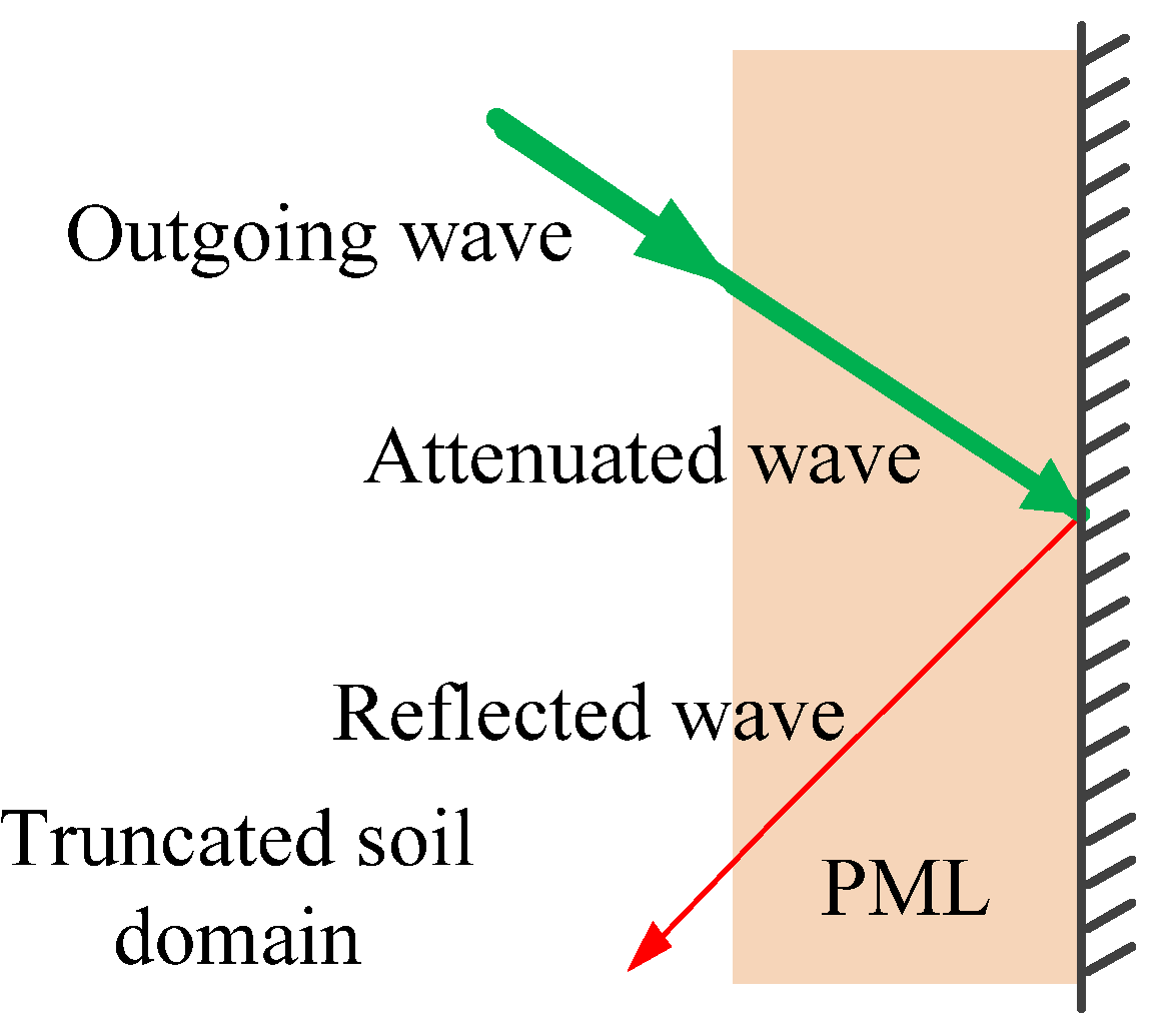
In dynamic analyses, the existence of artificial boundaries will create reflections of waves and contaminate the results. To solve this problem, the Perfectly Matched Layer (PML) is used in this study, which has been proved to be an efficient way for the bounded-domain modeling of wave propagation in unbounded domains. The PML is appropriate for explicit time integration in large-scale dynamic finite element analyses with accurate results and low computational costs [36]. As shown in Figure 9, the external manifestation of PML is a wave absorbing layer placed at the boundary of a truncated model which absorbs and attenuates waves propagating outward of the truncated model [37]. Assuming that the coordinate system is adopted to describe the 3D space and the coordinates system transformed from is supposed as the PML’s wave absorbing space, the stretching function can be expressed as (no summation) [31,33]:
where signifies the dimensionless frequency. The functions and work for attenuating the evanescent waves and the propagating waves, respectively. In practice, they can be chosen as , with , where is an optimal coefficient estimated from a pre-analysis; represents the distance into the PML and the is the direction of the PML depth. In LS-DYNA, the PML can be used with the material defined by the keyword *MAT_PML_ HYSTERETIC (Type 237) which is ad hoc for the material Type 232 used for soil in this finite element model.

Figure 9.
Perfectly Matched Layer (PML) artificial boundary.
Figure 9.
Perfectly Matched Layer (PML) artificial boundary.
Pore water pressure is considered in this study. In LS-DYNA, it can be treated as boundary conditions. In this study, the saturated and undrained conditions with normal mean high tide of 3.3 m are adopted, and they are applied in the model by using the corresponding keywords in LS-DYNA.
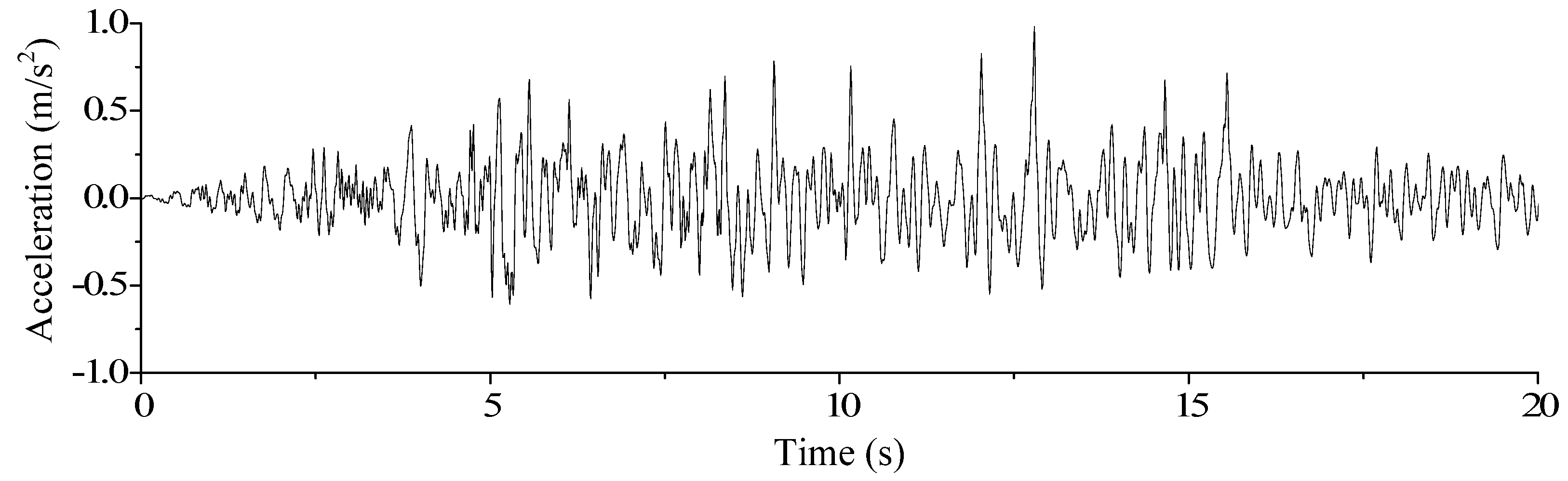
The input excitation in this study is the Shanghai artificial seismic wave record with the duration time of 20 s. The curve of acceleration versus time for the seismic motion imposed at the bedrock is shown in Figure 10. Since the seismic precautionary intensity of the tunnel is 7 degrees, the peak acceleration of 0.1 g, which can be obtained through the amplitude modulation, is required. Seismic impacts due to wave propagation—so called non-uniform seismic excitation—are considered here. As for the propagation direction, only the transverse one is taken into consideration. The seismic wave will propagate along the model from left to right. The horizontal acceleration excitation is imposed at the bottom of the model. The excitation has been imposed on the nodes at the bottom of the model at 5 m intervals with corresponding phase shifts, which reflect an apparent wave propagation velocity of 0.5 km/s from the island part to the land part.

Figure 10.
Shanghai artificial seismic input wave.
Figure 10.
Shanghai artificial seismic input wave.
3.5. Parallel Computing Environment
The Dawning 5000 A ranked 10th among the TOP 500 high performance computer list (November 2008) and is used as the parallel computing environment to conduct the simulation. This supercomputer with 233.5 TFlops as the peak value is suitable to be used to perform large-scale scientific computing, like the aseismic analysis of underground infrastructure.
The main system parameters of this supercomputer are shown in Table 2.
Table 2.
The parameters of the supercomputer Dawning 5000 A.
| Parameters | Value |
|---|---|
| Cores | 30720 |
| CPU | quad-core Opteron 8347 HE 1.9 GHz |
| Memory capacity | 95 TB |
| Storage capacity | 500TB SAN |
| Network | Infiniband connectX DDR |
| Operating system | SuSE-10.2 |
| Workload management platform | LSF 7.0 |
4. Results and Discussion
Before the seismic analysis, initial conditions like the geostress field were obtained by using the dynamic relaxation. When the stress and deformation of the soil-tunnel system became stable, the equilibrium configurations were obtained and the initial calculations were considered to complete. Then, the seismic analysis was performed. The simulation results and the parallel performance are discussed in the following subsections. Due to space limitations, without specific explanation only the west line tunnel is discussed here, while the east line can be analyzed in the same way.
4.1. Results Comparison and Method Validation
A series of studies on the earthquake-induced dynamic responses of the horizontal-cylindrical liquid vessels have been carried out by Karamanos [15,16]. Numerical solutions about the sloshing frequencies, the impulsive masses and the convective masses of the horizontal-cylindrical liquid storage tanks with respect to different liquid depths under longitudinal and transverse seismic excitation are obtained. Besides, an “equivalent rectangular container” method is proposed, which means that the externally induced dynamic responses of a horizontal-cylindrical container with arbitrary liquid depth can be computed quite accurately by replacing the cylindrical container with an equivalent rectangular container which has the same free-surface dimensions and owns the same liquid volume [15]. The effectiveness and correctness of this equivalence have been numerically [38] and experimentally [39] demonstrated. In this study this equivalence technique is adopted to demonstrate the practicability of the proposed ALE based FSI approach for the interaction between tunnel linings and inner water. Assuming that the inner diameter of the tunnel is r and the free-surface height of the liquid is h, based on the equivalence theorem, the height of the liquid (heq) in the equivalent rectangular container can be calculated using Equation (18). Figure 11 illustrates the layout of the equivalent relationship.
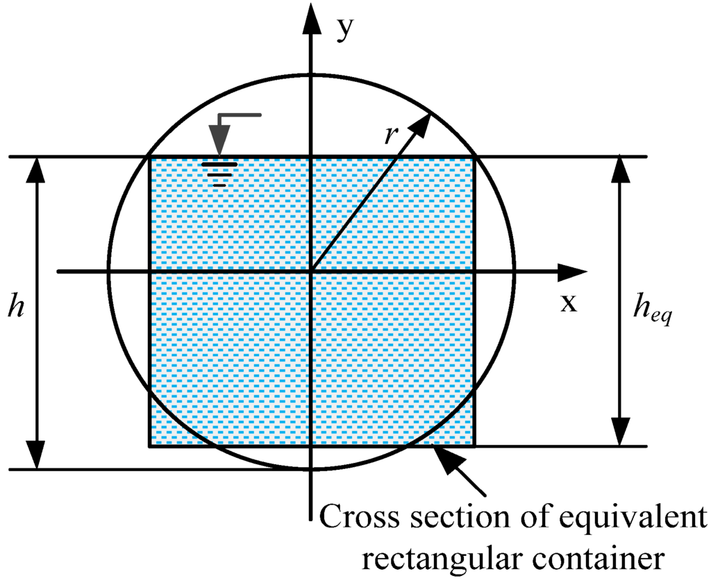
Figure 11.
Schematic layout of the equivalent relationship. r, h and heq mean the inner diameter of the tunnel, the free-surface height and the equivalent height, respectively.
Figure 11.
Schematic layout of the equivalent relationship. r, h and heq mean the inner diameter of the tunnel, the free-surface height and the equivalent height, respectively.

Once the cylindrical container is treated as its equivalent rectangular container, the equivalent masses can be calculated using the analytical solution proposed by Housner [12]. For liquid storage containers with rectangular cross section, the hydrodynamic pressure () along the height direction can be expressed as Equation (19), where can be expressed as Equation (20) and means the vertical coordinate of the location where the pressure is calculated. The equivalent mass attached to each node can be obtained by using the steps as follows. Firstly, through the mapping of equivalent rectangular surfaces and the original cylinder surface, the transformation of the pressure on the equivalent rectangular face to that on the original cylindrical face is completed. Then, the total equivalent mass on an element can be calculated by dividing the product which can be obtained through multiplying the area of the element’s face bearing pressure by the pressure value, by the current acceleration . At last, the obtained total equivalent mass is distributed to the four nodes owned by the element using Equation (21), where is the area of the face with pressure owned by the element; , means the equivalent mass at each node. Once the procedure is programmed, the whole finite element model can be processed automatically.
where
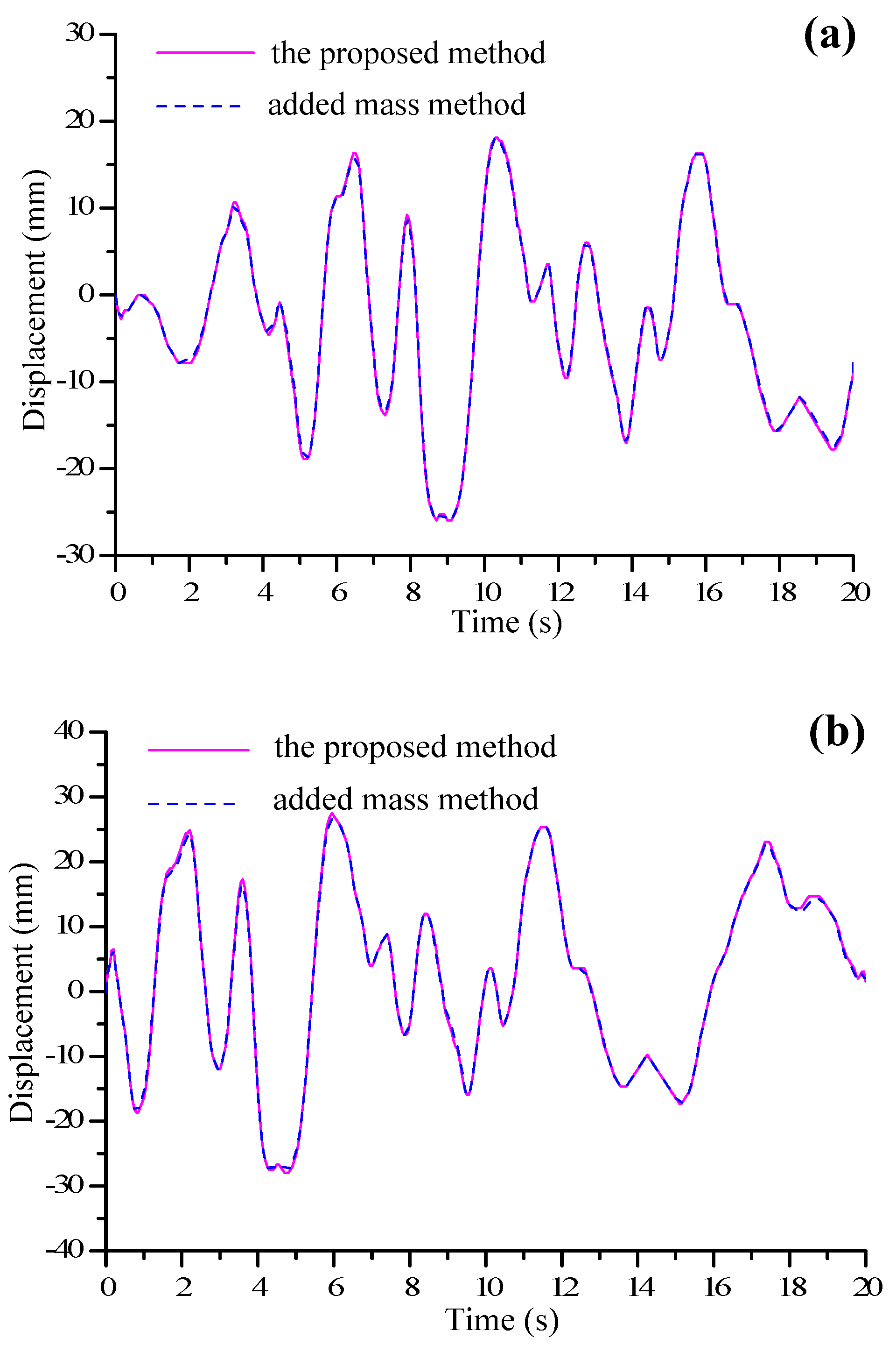
Without loss of generality, the free-surface height of the liquid is assumed to be 1.5r, where r is the diameter of the tunnel lining which is 2.75 m for island and land part and 2.92 m for cross river part. The equivalent masses are calculated and applied by using the above-mentioned procedure. Figure 12 illustrates the comparison of the lateral displacements under seismic excitation obtained by using the added mass method and the proposed ALE based fluid–structure interaction method at sections IS6 and RS6 (see Figure 7). It is seen that the variation law of the displacement shows good agreement and the displacement values are also very close to each other. While, at some points the displacement values from these two methods cannot fit perfectly and discrepancy exists. This is because the proposed method considers the sloshing of the fluid which is neglected by the added mass method. Besides, during the derivation of the added mass method the structure is assumed to be the rigid body without flexibility [40]; thus, it is considered that the results obtained from the proposed ALE based fluid–structure interaction method are closer to realistic conditions. Other sections show similar results. Thus, the correctness and reliability of the proposed ALE based fluid–structure interaction method for dealing with the coupling between the tunnel lining and inner water are verified.
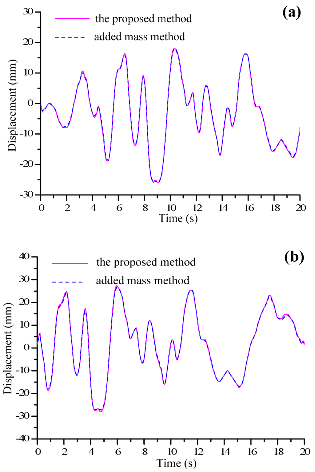
Figure 12.
Contrast of the displacement responses using the proposed method and the added mass method at sections: (a) IS6; (b) RS6. IS6 and RS6 mean the chosen section at the island part and the cross-river part, respectively.
Figure 12.
Contrast of the displacement responses using the proposed method and the added mass method at sections: (a) IS6; (b) RS6. IS6 and RS6 mean the chosen section at the island part and the cross-river part, respectively.
4.2. Dynamic Response Analysis
The seismic responses of a shield tunnel can be investigated in terms of three primary aspects, namely, extension/compression, longitudinal bending and ovaling [9]. In this study, the extension/compression can be recognized through the axial forces and the bending behavior can be evaluated through the bending moments; the ovaling deformation can be evaluated by measuring the diameter variation of the tunnel. In total, 24 typical cross-sections including nine in the island part, 10 in the cross-river part and five in the land part (as shown in Figure 7) are chosen as the concerned locations.
Figure 13 depicts the evolutions of dynamic internal forces and Figure 14 illustrates the evolutions of dynamic internal moments. The tunnel suffers alternately positive and negative dynamic forces and moments. Time history of internal forces of other sections show comparable results. To get a total view of internal forces, Figure 15 illustrates the variation of maximum axial forces along the tunnel and Figure 16 depicts that of the maximum bending moments. The obtained results show that both the bending moments and the axial forces change along the tunnel. Different internal forces and moments have been observed among the island part, cross-river part and land part. The differences may be attributed to the non-uniform seismic input model, the winding and different spatial positions of the tunnel, the dissimilar distributions of soil strata and the diverse buried depths of the tunnel. The comparison illustrates the distributions of both the internal moments and the internal forces of the tunnel during and after the earthquake, which can be used to aid the design of connections of different rings, connections of different segments in a ring and water-proof measures.
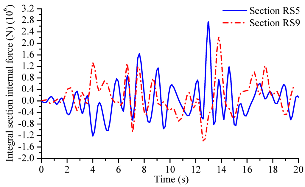
Figure 13.
Dynamic integral axial forces at sections RS5 and RS9. RS5 and RS9 mean the chosen sections at the cross-river part.
Figure 13.
Dynamic integral axial forces at sections RS5 and RS9. RS5 and RS9 mean the chosen sections at the cross-river part.

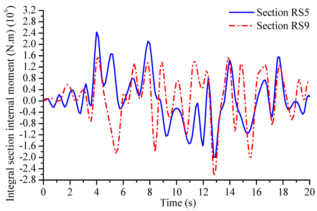
Figure 14.
Dynamic integral transverse moments at sections RS5 and RS9. RS5 and RS9 mean the chosen sections at the cross-river part.
Figure 14.
Dynamic integral transverse moments at sections RS5 and RS9. RS5 and RS9 mean the chosen sections at the cross-river part.


Figure 15.
Maximum integral axial forces along the tunnel.
Figure 15.
Maximum integral axial forces along the tunnel.
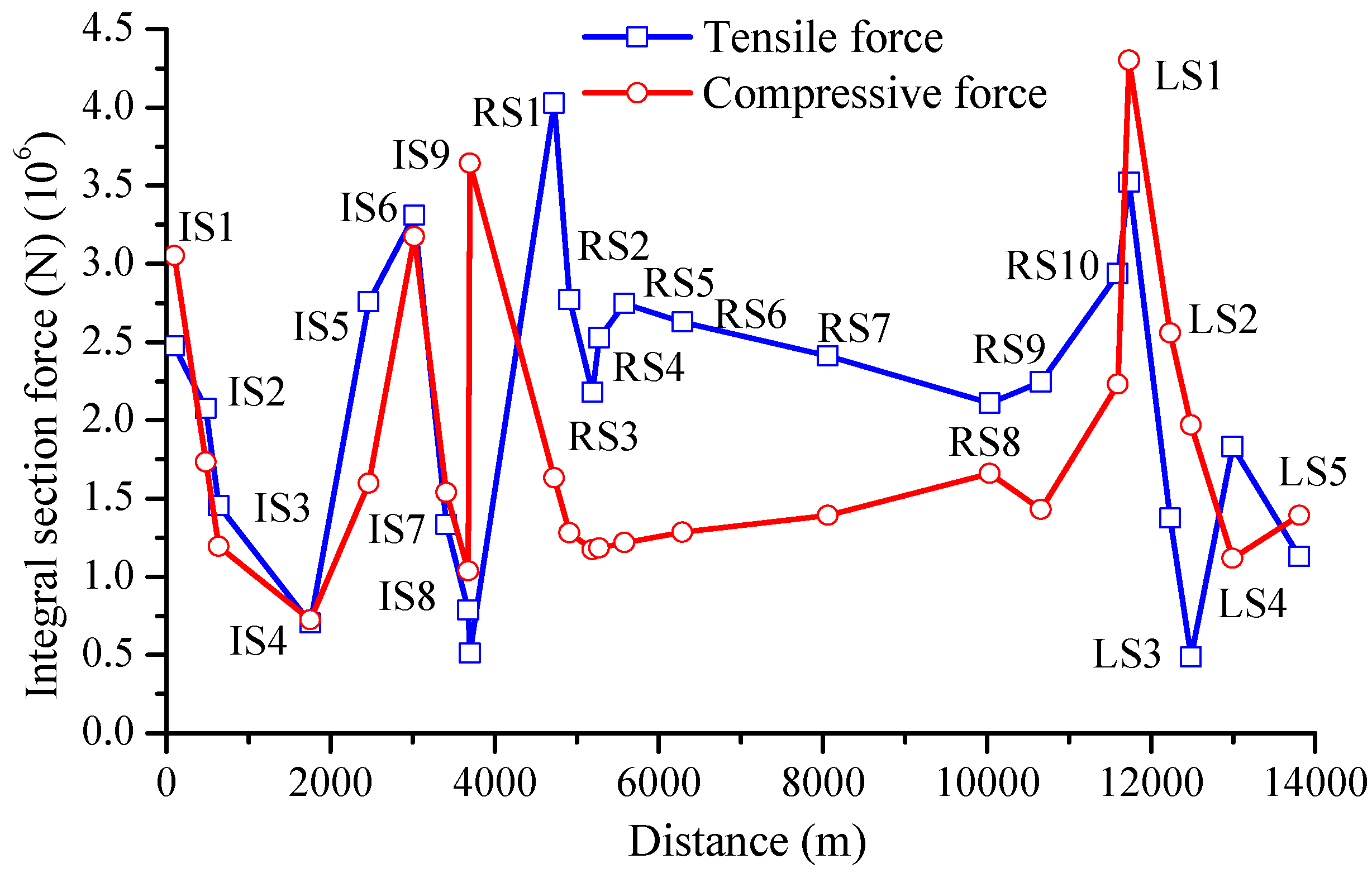
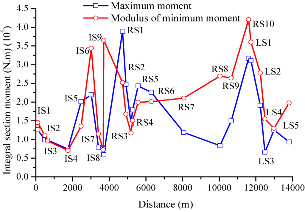
Figure 16.
Maximum integral transverse moments along the tunnel.
Figure 16.
Maximum integral transverse moments along the tunnel.

To evaluate the strength of the tunnel, the hoop stress is extracted and analyzed. As shown in Figure 17, the local coordinate system is needed in each typical cross-section to obtain the hoop stress. Figure 18 depicts the maximum compressive and tensile dynamic hoop stress distributions of cross-sections RS1 and RS5. It is shown that the distributions present similar patterns in different sections. The maximum stresses lie in the two sides of the ring, and the minimum stresses lie in the arc bottom and vault. Other sections show similar change laws. Table 3 lists the maximum hoop stress for the chosen sections. The hoop stress also changes along the tunnel, and the larger stress appears at sections IS1, IS5, IS6 and IS9 in the island part, sections RS1 and RS10 in the cross-river part, and section LS1 in the land part. The maximum compressive stress and the maximum tensile stress are 8.36 MPa and 5.32 MPa, respectively. The larger stresses may be due to the ovaling deformation of the tunnel and the sharp stiffness changes between the work shafts and the tunnel rings. Since the maximum compressive and tensile hoop stresses are smaller than the corresponding concrete strength used, the tunnel meets the strength design requirements under the specific seismic excitation.

Figure 17.
Local coordinate system: (a) local cylindrical coordinate; (b) hoop and axial stress.
Figure 17.
Local coordinate system: (a) local cylindrical coordinate; (b) hoop and axial stress.
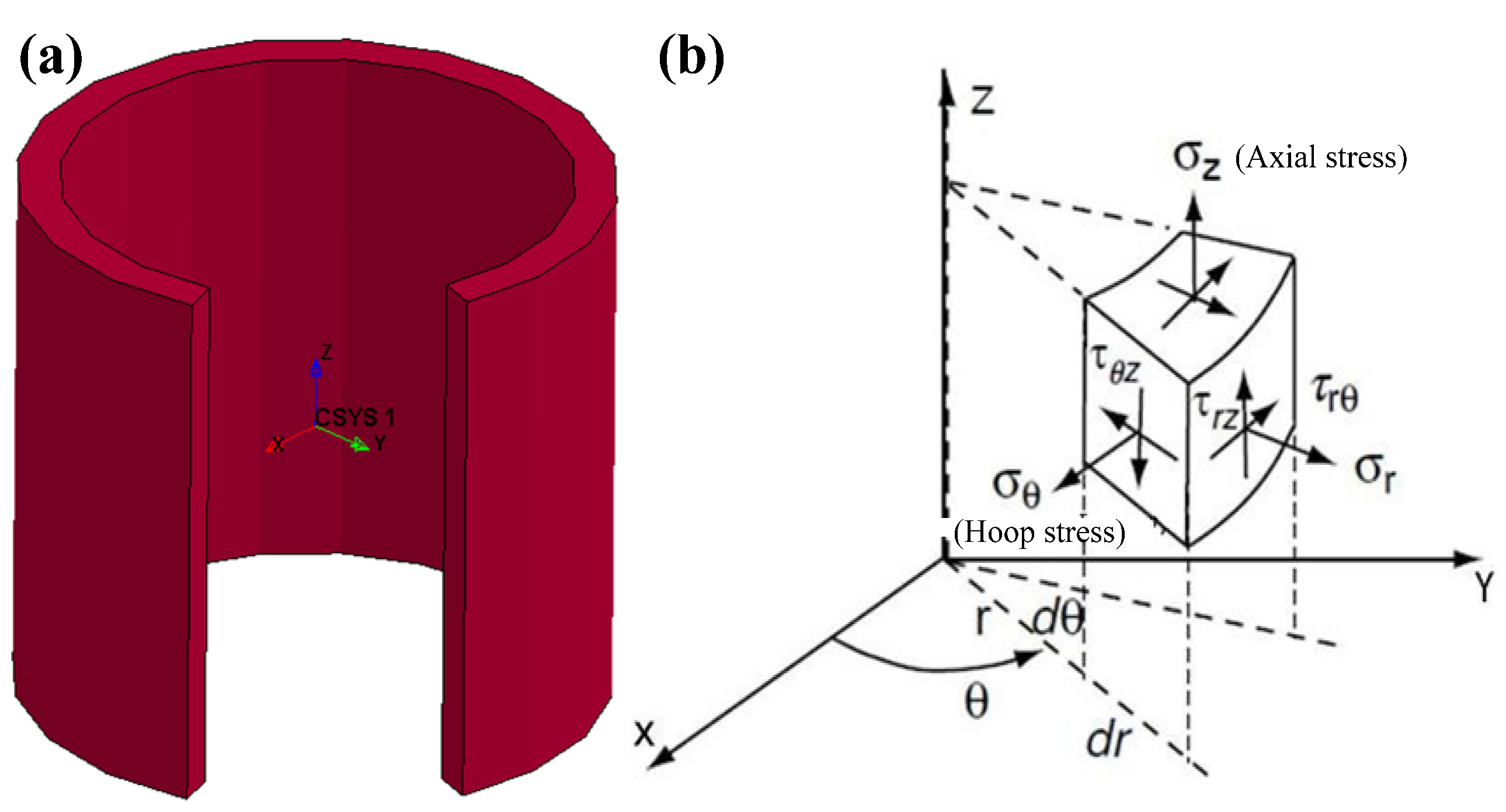

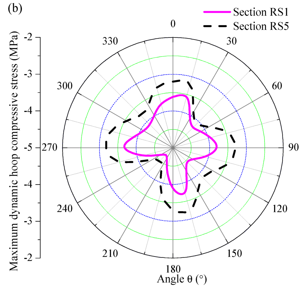
Figure 18.
Distributions of max dynamic hoop stresses around the tunnel lining during earthquake: (a) tensile; (b) compressive.
Figure 18.
Distributions of max dynamic hoop stresses around the tunnel lining during earthquake: (a) tensile; (b) compressive.
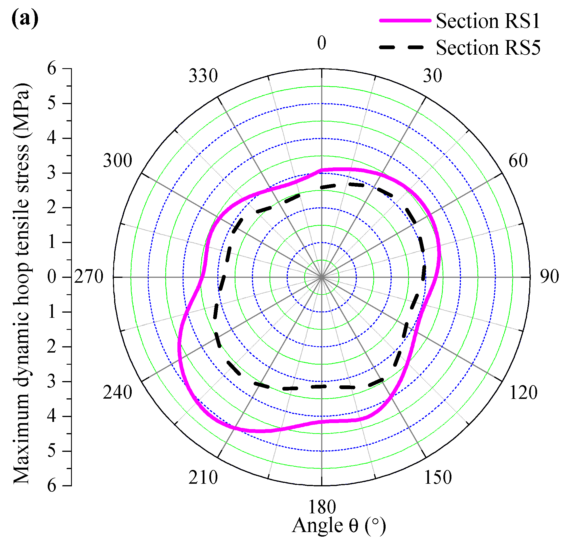

Table 3.
Maximum hoop stress of all control sections (MPa).
| Control Sections | IS1 | IS2 | IS3 | IS4 | IS5 | IS6 | IS7 | IS8 | IS9 | RS1 | RS2 | RS3 |
|---|---|---|---|---|---|---|---|---|---|---|---|---|
| Maximum compressive stress | 4.00 | 1.99 | 1.89 | 1.83 | 3.91 | 5.69 | 2.07 | 1.88 | 3.80 | 4.76 | 4.20 | 2.95 |
| Maximum tensile stress | 3.14 | 2.38 | 2.24 | 1.85 | 3.52 | 3.57 | 1.99 | 1.87 | 1.61 | 5.32 | 3.95 | 3.15 |
| Control sections | RS4 | RS5 | RS6 | RS7 | RS8 | RS9 | RS10 | LS1 | LS2 | LS3 | LS4 | LS5 |
| Maximum compressive stress | 4.05 | 4.55 | 4.58 | 4.65 | 5.39 | 5.27 | 8.36 | 6.17 | 5.52 | 4.09 | 3.82 | 1.71 |
| Maximum tensile stress | 3.29 | 3.76 | 3.71 | 3.07 | 2.04 | 2.92 | 5.20 | 4.22 | 3.47 | 1.77 | 3.09 | 2.11 |
Note: IS1–IS9, RS1–RS10 and LS1–LS5 depict the chosen control sections in the island, cross-river and land part, respectively.
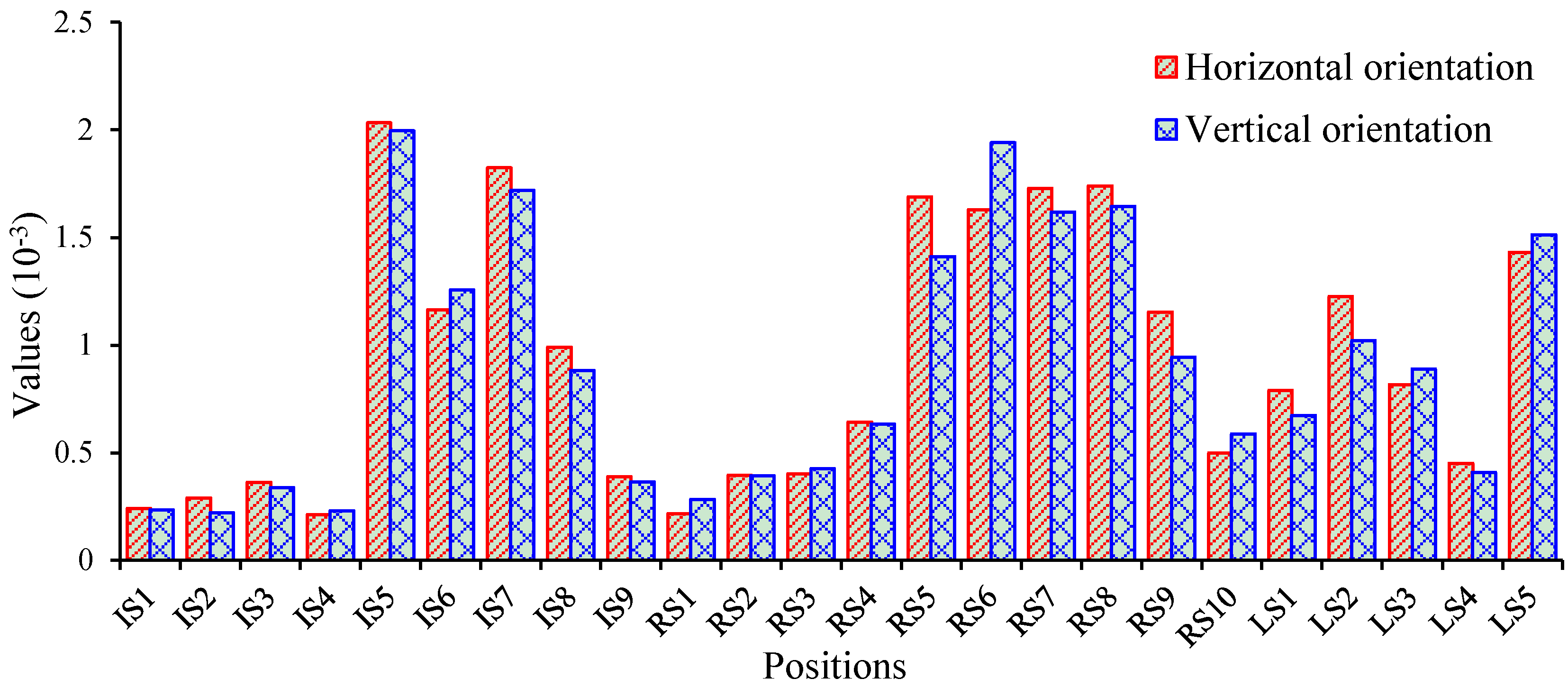
The ovaling describes the cross-sectional distortion of the tunnel lining and can be characterized by the change of the diameter. Thus, the ovaling here is defined by both the horizontal and the vertical diameter variations. Assuming that represents the horizontal and vertical variation rate of the tunnel lining, it can be expressed as , where and are the diameter of the tunnel before and after the deformation, respectively. Figure 19 represents the diameter variation of the tunnel lining at section RS6. Unlike the uniform excitation, pure shear deformation is not observed. This may be due to the non-uniform seismic input and the sophisticated SSI. Figure 20 shows the maximum variation of diameter for all cross-sections along the tunnel. The cross sections IS5, RS6 and LS5 bear larger deformations, which is partially due to the deeper buried depth. It is known that the ovaling deformation will cause additional dynamic stress concentrations in the tunnel linings and may cause damage to the tunnel during earthquakes. However, for this tunnel, from the aforementioned discussion, it can be stated that the hoop stress is below the strength limitation. Furthermore, from the discussion in this section it can be noted that the maximum ovaling deformation is less than 0.3%, which also satisfies the design requirements [41].
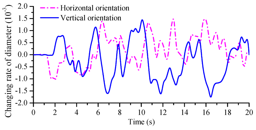
Figure 19.
History over time of diameter change rate at section RS6. RS6 depicts the chosen control sections in the cross-river part.
Figure 19.
History over time of diameter change rate at section RS6. RS6 depicts the chosen control sections in the cross-river part.


Figure 20.
Normalized maximum values of ovaling deformation at different cross sections (horizontal (+), vertical (−)).
Figure 20.
Normalized maximum values of ovaling deformation at different cross sections (horizontal (+), vertical (−)).
4.3. Domain Decomposition Comparison and Parallel Performance Evaluation
All simulations were carried out using the proposed MRCB (modified Recursive Coordinate Bisection) based parallel computing method, which was embedded in the LS-DYNA optimized to run on the Dawning 5000 A at the Shanghai Supercomputer Center. The evaluation of the developed parallel method applied in the seismic analysis of the specific water conveyance tunnel will be presented in this section.
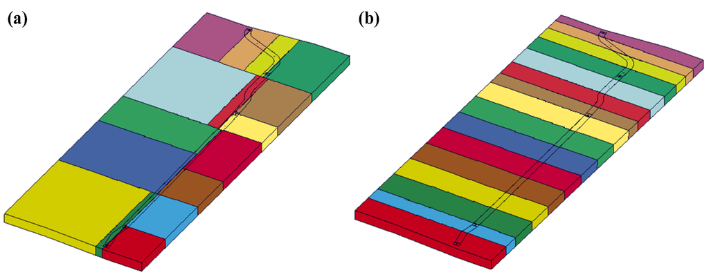
Figure 21.
Description of domain decomposition topology for 16 subdomains using: (a) recursive coordinate bisection (RCB) method; (b) modified recursive coordinate bisection (MRCB) method.
Figure 21.
Description of domain decomposition topology for 16 subdomains using: (a) recursive coordinate bisection (RCB) method; (b) modified recursive coordinate bisection (MRCB) method.

To evaluate the proposed MRCB domain decomposition method (DDM), calculations were carried out with 1, 2, 4, 8, 16 and 32 cores using RCB and MRCB, separately. The topologies of domain decomposition with 16 subdomains for the dynamic model using these two DDMs are shown in Figure 21. From this figure, one can easily find that the topologies from these two DDMs are different, more specifically, by using RCB the model is split in both x and y direction along which the model is longest, while by using MRCB the model is divided only in the, x direction along which the coupling (contact and FSI) load is distributed. Thus the MRCB may lead to a more balanced distribution of coupling loads from a qualitative perspective.
For further quantitative analyses of the differences between these two domain decomposition methods, Table 4 lists the load details (number of nodes participating in calculation) of each subdomain using these two methods, respectively. As shown in this table, for each subdomain of both these two DDMs, the total number of nodes (Ntol) is almost equal. However, the subdomains obtained from RCB have a very unbalanced distribution of nodes involved in contact (Ncon) and FSI (Nfsi), in contrast with those obtained from MRCB. As is known to all, the calculation overheads of nodes participating in contact or FSI far outweigh those of common nodes. Therefore, for the traditional RCB method, the loads of each partition cannot achieve balance, and cores processing partitions with heavier loads will take extra time when cores processing partitions with less loads are idle and waiting. As a result, the expensive computing resources are wasted and the total calculation time increases unnecessarily. On the contrary, the nodes in contact and the FSI of the partitions from the MRCB method are well distributed, and the number of these nodes in every subdomain is approximately equal. Therefore, the total loads in every subdomain are balanced. Besides, the running time of cores processing each subdomain is almost the same, so the computing resources are used fully and reasonably, and the total calculation time decreases greatly.
Table 4.
Comparison of domain decomposition results obtained by different approaches.
| Subdomain | RCB Method | MRCB Method | ||||
|---|---|---|---|---|---|---|
| Ntol | Ncon | Nfsi | Ntol | Ncon | Nfsi | |
| SD1 | 120,880 | 8828 | 5515 | 120,037 | 11,252 | 5790 |
| SD2 | 122,157 | 11,548 | 6188 | 121,002 | 11,067 | 5736 |
| SD3 | 117,797 | 17,873 | 10,480 | 119,524 | 11,133 | 5736 |
| SD4 | 116,319 | 0 | 0 | 119,577 | 11,074 | 5736 |
| SD5 | 121,399 | 14,339 | 6200 | 119,399 | 11,159 | 5736 |
| SD6 | 120,709 | 11,708 | 7334 | 119,378 | 10,871 | 5736 |
| SD7 | 118,680 | 14,120 | 6580 | 119,355 | 11,062 | 5735 |
| SD8 | 122,386 | 11,596 | 7206 | 119,342 | 11,059 | 5736 |
| SD9 | 121,623 | 12,545 | 6240 | 119,217 | 11,059 | 5736 |
| SD10 | 118,561 | 7497 | 4197 | 119,106 | 11,060 | 5735 |
| SD11 | 120,636 | 19,267 | 9257 | 118,645 | 11,058 | 5736 |
| SD12 | 116,330 | 0 | 0 | 119,413 | 11,059 | 5734 |
| SD13 | 118,108 | 11,736 | 5740 | 119,657 | 11,058 | 5736 |
| SD14 | 121,415 | 12,996 | 5514 | 120,054 | 11,063 | 5736 |
| SD15 | 120,924 | 16,128 | 8800 | 121,230 | 11,071 | 5739 |
| SD16 | 115,600 | 6719 | 2578 | 118,588 | 10,795 | 5736 |
Note: SD: Subdomain; RCB: recursive coordinate bisection; MRCB: modified recursive coordinate bisection; Ntol: the total number of nodes; Ncon: the number of nodes involved in contact in each SD; Nfsi: the number of nodes involved in FSI in each SD.
Table 5 shows the time consumption and parallel performance of different approaches with different numbers of cores to perform a 20 s real-time seismic analysis, where , and represent total computation time, speedup and parallel efficiency, respectively. As shown in the table, MRCB presents a more balanced load distribution and a higher speed up and parallel efficiency compared to those of RCB. Therefore, the total computation time decreases.
Table 5.
Scalability performance of different methods.
| Number of Cores | RCB Method | MRCB Method | ||||
|---|---|---|---|---|---|---|
| Ti (s) | Su | Ef (%) | Ti (s) | Su | Ef (%) | |
| 1 | 3,299,460 | 1 | 100 | 3,299,460 | 1 | 100 |
| 2 | 1,729,320 | 1.91 | 95.4 | 1,693,620 | 1.95 | 97.4 |
| 4 | 900,240 | 3.67 | 91.6 | 882,720 | 3.74 | 93.4 |
| 8 | 523,920 | 6.3 | 78.7 | 505,500 | 6.53 | 81.6 |
| 16 | 322,056 | 10.24 | 64 | 282,352 | 11.69 | 73 |
| 32 | 182,210 | 18.11 | 56.6 | 159,923 | 20.63 | 64.5 |
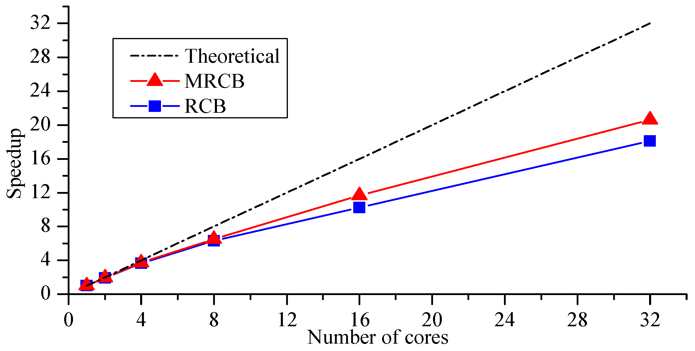
The comparison of speedup for the parallel dynamic analysis is also shown in Figure 22. The increment of speedup for both RCB and MRCB is not linearly proportional to the increment of cores involved in computation, which means that the parallel efficiency drops when the number of processor cores grow. Compared with RCB, the speedup of MRCB is larger and closer to the theoretical one and this superiority increases as the number of cores grows.

Figure 22.
Speedup of different parallel schemes.
Figure 22.
Speedup of different parallel schemes.
4.4. Parametric Study
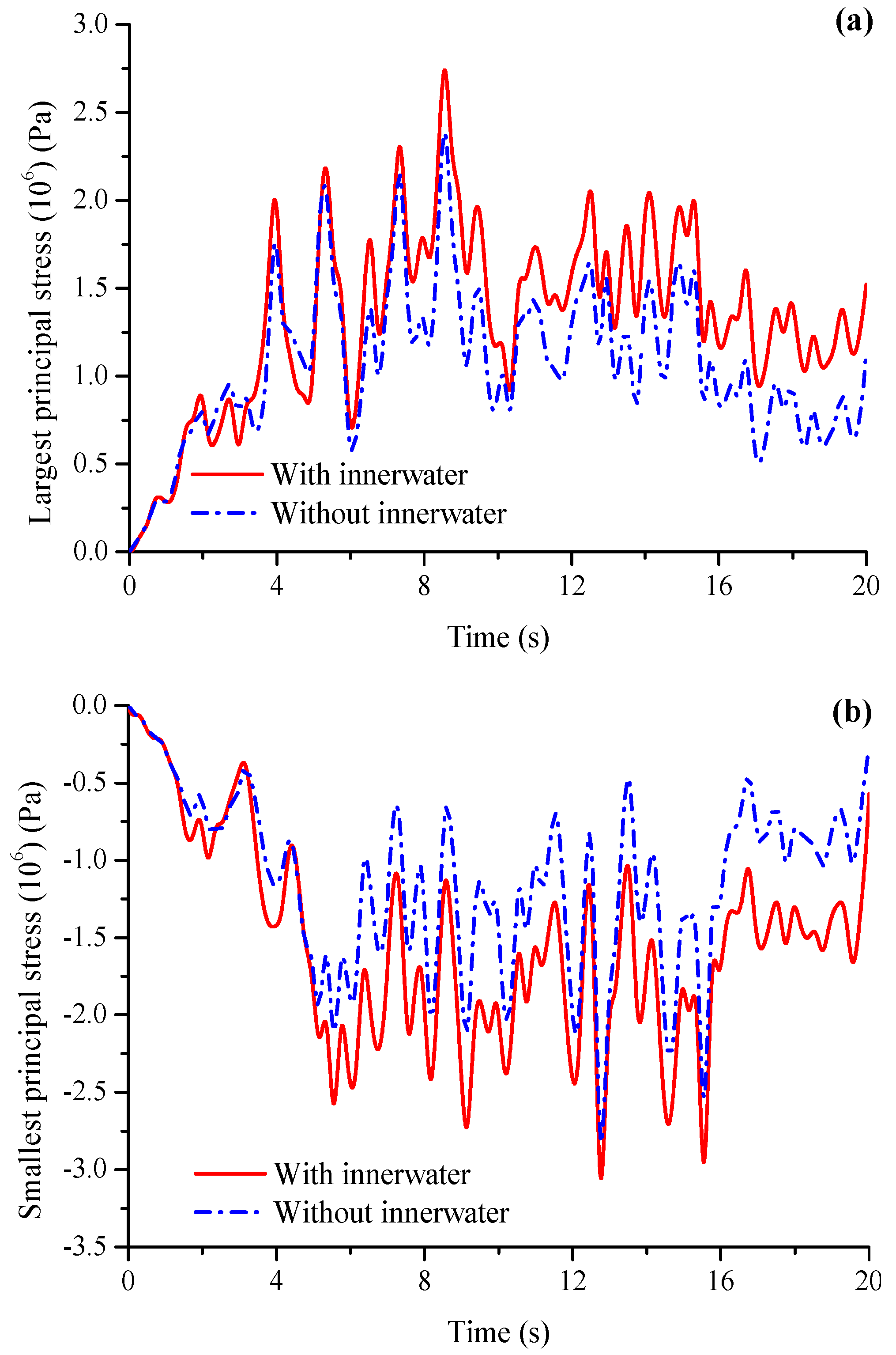
Different from common tunnels, water conveyance tunnels require special consideration. The interaction between inner water and the tunnel lining must be examined [23,42], as it will affect the dynamic responses of the tunnel during earthquakes. In this study, the tunnel with full water, corresponding to normal operation conditions, is considered. However, there are also other conditions like the modification condition with an empty tunnel and the water hammer condition. With the intention of comparing and evaluating the effects of the inner water on seismic responses of the tunnel, the double-line tunnel with no water inside under the same traveling seismic excitation is also analyzed using the proposed parallel algorithm. The parameters are the same as those illustrated in Section 3 except for the removed inner water. Figure 23 shows the comparison of the largest and smallest first order principal stresses of section RS5 during the earthquake. It is shown that the tunnel with inner water suffers higher stresses than those of the empty tunnel, which means that the existence of inner water may make the tunnel more vulnerable during earthquakes. These results may be attributed to the added mass, the sloshing of the inner water and the FSI between inner water and the tunnel. Other sections show similar trends. Therefore, the simulation of the water conveyance tunnel with filled water included by this paper’s study may give more reasonable guidelines for the tunnel design.

Figure 23.
Effects of the inner water on dynamic responses evaluated by principal stress: (a) the largest one; (b) the smallest one.
Figure 23.
Effects of the inner water on dynamic responses evaluated by principal stress: (a) the largest one; (b) the smallest one.
The deformation joints embedded in the tunnel can prevent the tunnel from being damaged by non-uniform subsidence and accidental external forces. They can also alleviate the stress concentrations caused by sharp changes of structure and stiffness when the tunnel is subjected to earthquakes. For this specific tunnel, three deformation joints are embedded to connect the tunnel lining ring and the work shaft. The layout of deformation joints is shown in Figure 8d. The effects of the deformation joints on the dynamic responses of the tunnel under seismic excitation are studied here using the established three-dimensional full scale model. Figure 24 illustrates the modulus of the maximum dislocation displacement of each deformation joint, namely, (see Figure 8d). For brevity, in this Figures S1–S5 represent the water sluice work shaft, middle work shaft, Changxing island work shaft, Pudong work shaft and Pudong #5 conduit work shaft, respectively; LE and RI mean the left side and the right side of each work shaft along the tunnel from S1 to S5, respectively; a, b and c denote the first, second and third deformation joint in the direction away from each work shaft, respectively (see Figure 8d). For instance, S1RIa means the first deformation joint at the right side of the water sluice work shaft. As shown in Figure 24, the maximum dislocation displacements of deformation joints situated in the same location at both two sides of a work shaft are close to each other; and for deformation joints at one side of a work shaft, the smaller the distance between the deformation joint and the work shaft is, the bigger the dislocation displacement becomes. Besides, the maximum dislocation displacement occurs at S3RIa and the maximum value is about 3 mm.
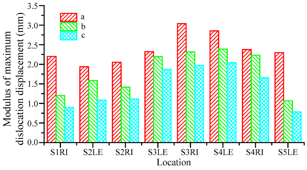
Figure 24.
Modulus of maximum dislocation displacement of each deformation joint.
Figure 24.
Modulus of maximum dislocation displacement of each deformation joint.

To further evaluate the function of the deformation joints, cases with and without deformation joints are considered. Table 6 shows the largest compressive stresses and the largest tensile stresses of the lining at two sides of each work shaft with and without deformation joints during earthquakes. It can be seen that with deformation joints the tensile and compressive stresses decrease and the maximum decrement appears at S3RI (right of the Changxing island work shaft) with a value of about 16.7%. By comparing with Figure 24, it is found that this is the exact location of the maximum dislocation displacement. Thus, it can be perceived that the dislocation of the deformation joints absorbs energy and causes the corresponding stresses to decrease. Therefore, the existence of deformation joints makes the shear deformation of tunnel linings occur at two sides of the deformation joints, and thus partially releases the stress of the tunnel linings near work shafts.
Table 6.
Effect of the deformation joints on maximum stresses of the tunnel.
| Location | Largest Tensile Stress | Largest Compressive Stress | ||||
|---|---|---|---|---|---|---|
| Without | With | Change (%) | Without | With | Change (%) | |
| S1RI | 1.698 | 1.548 | −8.83 | 1.716 | 1.610 | −6.18 |
| S2LE | 1.208 | 1.125 | −6.87 | 1.222 | 1.157 | −5.32 |
| S2RI | 1.266 | 1.176 | −7.11 | 1.526 | 1.429 | −6.36 |
| S3LE | 1.894 | 1.718 | −9.29 | 2.861 | 2.538 | −11.29 |
| S3RI | 2.634 | 2.194 | −16.7 | 2.793 | 2.349 | −15.9 |
| S4LE | 3.027 | 2.661 | −12.09 | 2.841 | 2.383 | −16.12 |
| S4RI | 2.548 | 2.278 | −10.6 | 2.838 | 2.568 | −9.51 |
| S5LE | 2.589 | 2.348 | −9.31 | 2.730 | 2.487 | −8.9 |
5. Conclusions
Seismic disasters may cause tunnel damage and contaminate the potable water system. Aseismic analyses of water conveyance tunnels are essential. To evaluate the aseismic ability of water conveyance tunnels, this paper presents the full scale three-dimensional nonlinear finite element model of a large-scale water conveyance tunnel and a series of numerical tests. The ALE algorithm is used to simulate the movement and deformation of the inner water. The nonlinear interaction between tunnel and inner water is dealt with by the penalty method. Though the numerical simulation is one effective method to evaluate the tunnel stability during earthquakes, it is generally difficult to carry out an analysis of the full scale, three-dimensional tunnel because of computing power limitations. To solve this problem, the MRCB based parallel computing method has been developed in this paper. Based on this proposed method, the full scale, three-dimensional dynamic responses of the water conveyance tunnel under seismic actions is investigated. The numerical approaches and the model are validated by a comparison with the added mass method. Dynamic responses of the tunnel are analyzed and the parallelism is discussed. Besides, factors affecting dynamic responses are investigated. From this study, the conclusions are drawn as follows:
- (1)
- The ALE based FSI method can be used to deal with the interaction between tunnel lining and inner water. The approaches and the established model in this study are suitable for the seismic analyses of the large-scale water conveyance tunnel and can be used as an effective way for performing seismic analyses of analogous tunnels.
- (2)
- The proposed MRCB domain decomposition method considers the features of the underground tunnel and the balance between time-consuming contact and FSI coupling loads. The proposed MRCB based parallel computing method has a higher speedup and a better parallel efficiency than that of the RCB based method. The proposed MRCB based parallel computing method can accelerate the calculation process of the nonlinear dynamic analyses for large-scale water conveyance tunnels under seismic excitation. The proposed parallel technique makes the simulation of large-scale models more efficient and provides an effective approach for numerical simulation of large-scale underground infrastructure.
- (3)
- The water conveyance tunnel fulfills the design requirements under seven degree seismic intensity. The results for axial forces, moments, stresses and deformations show its earthquake resistance. The simulation results can be used as references for the anti-seismic design of large-scale water conveyance tunnels. Specifically, the internal forces and moments obtained during and after the earthquake can be used to aid the design of connections for different rings, connections of different segments in a ring and water-proof measures, and the stresses and deformations obtained can be employed to evaluate the strength and stiffness of the tunnel structures.
- (4)
- The tunnel with filled water suffers higher stresses compared to the empty tunnel. The amount of inner water should be considered during the design and analyses of water conveyance tunnels. The deformation joints can partially release the stresses of the tunnel linings near work shafts caused by the sharp changes of structure and stiffness during earthquakes.
Future work includes the optimization of the proposed parallel method to improve its scalability performance.
Acknowledgments
The study is financially supported by 863 Program (number 2012AA01AA307) of China and the Natural Science Foundation Program (numbers 51475287 and 11272214) of China. The authors thank the Shanghai Supercomputer Center and the Shanghai Qingcaosha Investment Construction & Development Co. Ltd. for help and support.
Author Contributions
All of the authors discussed and proposed the analysis method, and analyzed the data. Xiaoqing Wang established the analysis model, accomplished the computation and wrote the paper; Xianlong Jin performed the validation of the analysis method and evaluated the parallel efficiency with the help from Puyong Wang; Zhihao Yang provided the design material and guidelines for analyses of the applied tunnel engineering project.
Conflicts of Interest
The authors declare no conflict of interest.
References
- Cheng, X.; Xu, W.; Yue, C.; Du, X.; Dowding, C.H. Seismic response of fluid–structure interaction of undersea tunnel during bidirectional earthquake. Ocean Eng. 2014, 75, 64–70. [Google Scholar] [CrossRef]
- Sahoo, J.P.; Kumar, J. Seismic stability of a long unsupported circular tunnel. Comp. Geotech. 2012, 44, 109–115. [Google Scholar] [CrossRef]
- Yue, Q.; Ang, A.H.-S. Nonlinear response and reliability analysis of tunnels under strong earthquakes. Struct. Infrastruct. Eng. 2015, in press. [Google Scholar]
- Wang, Z.; Zhang, Z. Seismic damage classification and risk assessment of mountain tunnels with a validation for the 2008 Wenchuan earthquake. Soil Dyn. Earthq. Eng. 2013, 45, 45–55. [Google Scholar] [CrossRef]
- Menkiti, C.; Mair, R.; Miles, R. Highway tunnel performance during the 1999 duzce earthquake. In Proceedings of the 15th International Conference on Soil Mechanics and Geotechnical Engineering, Istanbul, Turkey, 28–31 August 2001.
- Wang, J.N. Seismic Design of Tunnels: A Simple State-of-the-Art Design Approach; Parsons Brinckerhoff Quade & Douglas: New York, NY, USA, 1993. [Google Scholar]
- Stamos, A.; Beskos, D. 3-D seismic response analysis of long lined tunnels in half-space. Soil Dyn. Earthq. Eng. 1996, 15, 111–118. [Google Scholar] [CrossRef]
- Ding, J.-H.; Jin, X.-L.; Guo, Y.-Z.; Li, G.-G. Numerical simulation for large-scale seismic response analysis of immersed tunnel. Eng. Struct. 2006, 28, 1367–1377. [Google Scholar] [CrossRef]
- Hashash, Y.M.; Hook, J.J.; Schmidt, B.; John, I.; Yao, C. Seismic design and analysis of underground structures. Tunn. Undergr. Space Technol. 2001, 16, 247–293. [Google Scholar] [CrossRef]
- Carter, J.P.; Desai, C.S.; Potts, D.M.; Schweiger, H.F.; Sloan, S.W. Computing and computer modelling in geotechnical engineering. In Proceedings of the ISRM International Symposium, Melbourne, Australia, 12–14 November 2000.
- Westergaard, H.M. Water pressures on dams during earthquakes. Trans. Am. Soc. Civ. Eng. 1933, 98, 418–432. [Google Scholar]
- Housner, G.W. Dynamic pressures on accelerated fluid containers. Bull. Seismol. Soc. Am. 1957, 47, 15–35. [Google Scholar]
- Ruiz, R.; Lopez-Garcia, D.; Taflanidis, A. An efficient computational procedure for the dynamic analysis of liquid storage tanks. Eng. Struct. 2015, 85, 206–218. [Google Scholar] [CrossRef]
- Budiansky, B. Sloshing of liquids in circular canals and spherical tanks. J. Aerosp. Sci. 1958, 27, 161–173. [Google Scholar] [CrossRef]
- Karamanos, S.A.; Patkas, L.A.; Platyrrachos, M.A. Sloshing effects on the seismic design of horizontal-cylindrical and spherical industrial vessels. J. Press. Vessel Technol. 2006, 128, 328–340. [Google Scholar] [CrossRef]
- Karamanos, S.A.; Papaprokopiou, D.; Platyrrachos, M.A. Finite element analysis of externally-induced sloshing in horizontal-cylindrical and axisymmetric liquid vessels. J. Press. Vessel Technol. 2009, 131. [Google Scholar] [CrossRef]
- Cao, Y.; Wang, P.Y.; Jin, X.L. Dynamic analysis of flexible container under wind actions by ALE finite-element method. J. Wind Eng. Ind. Aerodyn. 2010, 98, 881–887. [Google Scholar]
- Zhao, C.; Chen, J.; Xu, Q. Fsi effects and seismic performance evaluation of water storage tank of AP1000 subjected to earthquake loading. Nucl. Eng. Des. 2014, 280, 372–388. [Google Scholar] [CrossRef]
- Razzaq, M.; Damanik, H.; Hron, J.; Ouazzi, A.; Turek, S. FEM multigrid techniques for fluid–structure interaction with application to hemodynamics. Appl. Numer. Math. 2012, 62, 1156–1170. [Google Scholar] [CrossRef]
- Turek, S.; Hron, J.; Madlik, M.; Razzaq, M.; Wobker, H.; Acker, J.F.; Bungartz, H.; Mehl, M.; Schäfer, M. Numerical simulation and benchmarking of a monolithic multigrid solver for fluid–structure interaction problems with application to hemodynamics. In Fluid–Structure Interaction II: Modelling, Simulation, Optimization; Barth, T.J., Griebel, M., Keyes, D.E., Nieminen, R.M., Roose, D., Schlick, T., Eds.; Springer: Berlin, Germany, 2010; pp. 193–220. [Google Scholar]
- Turek, S.; Hron, J.; Razzaq, M.; Schäfer, M.; Bungartz, H.; Mehl, M.; Schäfer, M. Numerical benchmarking of fluid–structure interaction: A comparison of different discretization and solution approaches. In Fluid–Structure Interaction II: Modelling, Simulation, Optimization; Barth, T.J., Griebel, M., Keyes, D.E., Nieminen, R.M., Roose, D., Schlick, T., Eds.; Springer: Berlin, Germany, 2010; pp. 413–424. [Google Scholar]
- Dupros, F.; de Martin, F.; Foerster, E.; Komatitsch, D.; Roman, J. High-performance finite-element simulations of seismic wave propagation in three-dimensional nonlinear inelastic geological media. Parallel Comput. 2010, 36, 308–325. [Google Scholar] [CrossRef]
- Chen, J.-Y.; Liu, J.-Y. Fluid–structure coupling analysis of water conveyance tunnel subjected to seismic excitation. Rock Soil Mech. 2006, 27, 1077. (In Chinese) [Google Scholar]
- Hou, G.; Wang, J.; Layton, A. Numerical methods for fluid–structure interaction—A review. Commun. Comput. Phys. 2012, 12, 337–377. [Google Scholar] [CrossRef]
- Razzaq, M. Finite Element Simulation Techniques for Incompressible Fluid–Structure Interaction with Applications to Bio-Engineering and Optimization. Ph.D. Thesis, TU Dortmund University, North Rhine-Westphalia, Germany, 16 February 2011. [Google Scholar]
- Sedarat, H.; Kozak, A.; Hashash, Y.M.; Shamsabadi, A.; Krimotat, A. Contact interface in seismic analysis of circular tunnels. Tunn. Undergr. Space Technol. 2009, 24, 482–490. [Google Scholar] [CrossRef]
- Kouretzis, G.P.; Sloan, S.W.; Carter, J.P. Effect of interface friction on tunnel liner internal forces due to seismic s-and p-wave propagation. Soil Dyn. Earthq. Eng. 2013, 46, 41–51. [Google Scholar] [CrossRef]
- Belytschko, T.; Liu, W.K.; Moran, B.; Elkhodary, K. Nonlinear Finite Elements for Continua and Structures; John Wiley & Sons Ltd.: New York, NY, USA, 2013. [Google Scholar]
- Xu, J.; Zou, J. Some nonoverlapping domain decomposition methods. SIAM Rev. 1998, 40, 857–914. [Google Scholar] [CrossRef]
- Bamford, T. An implementation of domain decomposition by recursive bisection. Available online: https://static.ph.ed.ac.uk/dissertations/hpc-msc/2006-2007/6547365-27d-d07rep1.2.pdf (accessed on 30 March 2015).
- Bernaud, D.; Maghous, S.; de Buhan, P.; Couto, E. A numerical approach for design of bolt-supported tunnels regarded as homogenized structures. Tunn. Undergr. Space Technol. 2009, 24, 533–546. [Google Scholar] [CrossRef]
- Felhös, D. Dry Sliding and Rolling Tribotests of Carbon Black Filled Epdm Elastomers and Their FE Simulations. Ph.D. Thesis, University of Kaiserslautern, Kaiserslautern, Germany, 16 December 2008. [Google Scholar]
- Spanos, P.D.; Tsavachidis, S. Deterministic and stochastic analyses of a nonlinear system with a biot visco-elastic element. Earthq. Eng. Struct. Dyn. 2001, 30, 595–612. [Google Scholar] [CrossRef]
- Pinto, P.A. Study of Constitutive Models for Soils under Cyclic Loading. Master’s Thesis, Universidade Técnica de Lisboa, Lisbon, Portugal, 12 November 2012. [Google Scholar]
- Livermore Software Technology Corporation. LS-DYNA Theory Manual. Available online: http://www.lstc.com/download/manuals (accessed on 5 November 2014).
- Zhu, J.; Taylor, Z.; Zienkiewicz, O. The Finite Element Method: Its Basis and Fundamentals; Butterworth-Heinemann: Oxford, UK, 2005. [Google Scholar]
- Basu, U. Explicit finite element perfectly matched layer for transient three-dimensional elastic waves. Int. J. Numer. Methods Eng. 2009, 77, 151. [Google Scholar] [CrossRef]
- Platyrrachos, M.; Karamanos, S. Finite element analysis of sloshing in horizontal-cylindrical industrial vessels under earthquake loading. In Proceedings of the ASME 2005 Pressure Vessels and Piping Conference, Denver, CO, USA, 17–21 July 2005.
- Abramson, H.N. The Dynamic Behavior of Liquids in Moving Containers; Report NASA-SP-106; Southwest Research Institute: San Antonio, TX, USA, 1966. [Google Scholar]
- Mircevska, V.; Bulajić, I.; Manova, K. Comparison of added mass method with sophisticated analytical BEM-FEM approach using ADAD-IZIIS software. In Proceedings of the 15th World Conference on Earthquake Engineering, Lisbon, Portugal, 24–28 September 2012.
- Shanghai Urban Construction and Communications Commission. Foundation Design Code (DGJ08–11–1999); Shanghai Urban Construction and Communications Commission: Shanghai, China, 1999. (In Chinese) [Google Scholar]
- Westfall, D.E. Water Conveyance Tunnels. In Tunnel Engineering Handbook; Springer: New York, NY, USA, 1996; pp. 298–310. [Google Scholar]
© 2016 by the authors; licensee MDPI, Basel, Switzerland. This article is an open access article distributed under the terms and conditions of the Creative Commons by Attribution (CC-BY) license (http://creativecommons.org/licenses/by/4.0/).