Article

Influence of Road Excitation and Steering Wheel Input on Vehicle System Dynamic Responses

1
School of Mechanical Engineering, Beijing Institute of Technology, Beijing 100081, China
2
LAMIH UMR CNRS 8201, University of Valenciennes, 59314 Valenciennes, France
3
College of Mechanical Engineering & Applied Electronics Technology, Beijing University of Technology, Beijing 100024, China
*
Author to whom correspondence should be addressed.
Appl. Sci. 2017, 7(6), 570; https://doi.org/10.3390/app7060570
Submission received: 23 March 2017 / Revised: 9 May 2017 / Accepted: 26 May 2017 / Published: 2 June 2017
(This article belongs to the Section Mechanical Engineering)

Abstract

:
Considering the importance of increasing driving safety, the study of safety is a popular and critical topic of research in the vehicle industry. Vehicle roll behavior with sudden steering input is a main source of untripped rollover. However, previous research has seldom considered road excitation and its coupled effect on vehicle lateral response when focusing on lateral and vertical dynamics. To address this issue, a novel method was used to evaluate effects of varying road level and steering wheel input on vehicle roll behavior. Then, a 9 degree of freedom (9-DOF) full-car roll nonlinear model including vertical and lateral dynamics was developed to study vehicle roll dynamics with or without of road excitation. Based on a 6-DOF half-car roll model and 9-DOF full-car nonlinear model, relationship between three-dimensional (3-D) road excitation and various steering wheel inputs on vehicle roll performance was studied. Finally, an E-Class (SUV) level car model in CARSIM® was used, as a benchmark, with and without road input conditions. Both half-car and full-car models were analyzed under steering wheel inputs of 5°, 10° and 15°. Simulation results showed that the half-car model considering road input was found to have a maximum accuracy of 65%. Whereas, the full-car model had a minimum accuracy of 85%, which was significantly higher compared to the half-car model under the same scenario.

1. Introduction

Vehicle roll behavior plays an important role in vehicle safety. Vehicle roll and rollover has been recognized as a vehicle crash type with the highest fatality. According to the National Highway Traffic Safety Administration (NHTSA) [1], vehicle roll or rollover occurred in 3% of all passenger-vehicle crashes in 2002, and 33% of all fatalities were related to vehicle roll. Although number of fatalities has been reduced over the last ten years, roll behavior still accounts for a large proportion of all deaths [2]. Hence, it is essential to carry out an in-depth study to understand vehicle roll behavior, which allows further improvement in passenger safety.
In recent years, studies reported in literature on vehicle roll behavior have mainly focused on detection systems and prevention/control algorithms. Yim [2] proposed a 3 degree of freedom (3-DOF) vehicle roll model to design a robust controller to prevent rollover and demonstrated effectiveness of the controller to prevent rollover using simulation with the nonlinear multi-body dynamics simulation CARSIM® software. Yi et al. [3] proposed an estimator based on a 3-DOF vehicle roll model and a 4-DOF half-car suspension model to obtain vehicle roll angle and roll rate while driving. In addition, a rollover index was used to indicate rollover danger, which was computed using measured lateral acceleration and yaw rate estimated roll angle and roll rate. Rajamani et al. [4,5] proposed a sensor fusion algorithm based on a 3-DOF vehicle roll model to estimate roll angle and center of gravity (C.G.) height. Experimental data was used to confirm performance reliability of developed algorithms in different maneuvers such as constant steering, ramp steering, double lane change and sine with dwell steering tests. Chen et al. [6] proposed an anti-rollover control algorithm based on a 3-DOF vehicle roll model to calculate Time-To-Rollover (TTR) in real-time. Larish et al. [7] developed a new predictive lateral load transfer ratio (PLTR) based a 4-DOF vehicle roll model, which utilized the driver’s steering input and several other sensor signals available from the vehicle’s electronic stability control system. This new PLTR index provided a time-advanced measurement of rollover propensity, thereby, offering significant benefits for closed-loop rollover prevention. Imine et al. [8] proposed an approach based on a 5-DOF vehicle roll model to estimate vertical forces affecting a vehicle using high-order sliding-mode (HOSM) observes. Employing previously estimated vertical forces; lateral rollover indicating rollover status was determined. Westhuizen et al. [9] proposed possibility of using slow active suspension control to reduce body roll and thus reducing rollover propensity. From the previous work reported in literature, it can be showed that an accurate model is required to approximate actual behavior.
From the discussion above, it can be seen that a majority of the vehicle roll dynamics models were established without considering road excitation and its coupling effects between vertical and lateral dynamics, i.e., no road input. This is in fact an important factor, as real roads are complex and in practice vehicle movements should be considered as variants.
To solve the above-mentioned problems, following two contributions are taken into account in this paper:
  • Influence of three-dimensional (3-D) road profile excitation on vehicle lateral and vertical coupling model is studied using half-car and full-car roll models.
  • Coupling relationship between the lateral and vertical dynamics using full car models is illustrated for various steering wheel step angle inputs and different road excitation conditions.
The above contributions were validated using CARSIM®, which has a high-fidelity nonlinear 9-DOF vehicle model.
In this paper, a comprehensive analysis considering road excitation and steering wheel input for vehicle roll behavior based on a 6-DOF half-car and a 9-DOF full-car model is proposed. For this analysis, first, a 3-D road profile based on power spectral density (PSD) was developed under straight and steering conditions. Next, 6-DOF and 9-DOF models were constructed under various road conditions. Then, vehicle roll responses using proposed models were obtained with or without the presence of road excitation and various steering wheel input. Finally, CARSIM® was utilized to validate the proposed 6-DOF and 9-DOF models. Results show that vehicle roll performance of 9-DOF model had a significantly higher accuracy than the 6-DOF roll model, especially in presence of road excitation and large steering wheel input.
In order to further illustrate functional relationships between road excitation and vehicle dynamics model, an approach which formulates a relationship between road level and steering wheel input is formulated in this paper. The paper is organized as follows. In Section 2, a 3-D road profile excitation model is briefly presented. Rollover index is illustrated in Section 3. In Section 4, vehicle dynamics of 6-DOF and 9-DOF models are studied. Section 5 deals with validation of the proposed models using CARSIM® for various road excitations and different steering wheel input. Finally, Section 6 concludes the paper.

2. Road Excitation Model

2.1. Parameter Optimization for Power Spectral Density

Distance between road surface and base plate is typically defined as a function of road irregularities. Road profile is typically assumed to be homogeneous and isotropic Gaussian random process, and its statistical characteristics can be described by PSD. According to the International Standards Organization (ISO) 8601 [10], PSD of road roughness can be defined as Equation (1).
G q ( n ) = G q ( n 0 ) ( n n 0 ) w
where n is spatial frequency in m 1 , n 0 is reference spatial frequency with a value of 0.1 m 1 , G q ( n 0 ) is PSD value for reference spatial frequency in m 3 , w is termed waviness, and reflects approximate frequency structure of the road profile, commonly taken as w = 2 . Also, G q ( n 0 ) represents different road levels ranging from A (very good) to H (very poor), depending on its values.
Equation (1) leads to estimation errors (overrated phenomenon) especially at low frequencies. To deal with this problem, PSD of road roughness based on rational white noise signal is proposed [11], and Equation (1) can be modified as follows.
G q ( n ) = α ρ 2 π ( α 2 + n 2 )
where α is constant related to road feature; ρ 2 represents variance of road roughness and n is spatial frequency in m 1 . More details are stated in [12].
Time domain representation of the road can be given as [11].
q ˙ ( t ) = α v q ( t ) + w ( t )
where, v represents velocity of the vehicle in m/s and w(t) is the white noise sequence. Covariance of white noise can be obtained as follows.
cov [ w ( t ) ] = E [ w ( t ) w ( t + τ ) ] = 2 ρ 2 α v δ ( τ )
where τ represents time-shift in s and δ(τ) is impulse function.
Then, the method of Least squares nonlinear parameter estimation is used to optimize the road parameters, and the following equation was utilized.
J = i = 1 N [ Φ ( n i , α , ρ ) G q ( n i ) ] 2 min
where N is the number of spatial frequency and ni is the sampling frequency points.
Using the ISO-8601 [10], we know that PSD of road roughness is four times for adjacent road levels. We obtain information to other road information based on one of them road parameter.
Based on the above analysis, optimal parameters for varying road level are listed in Table 1.
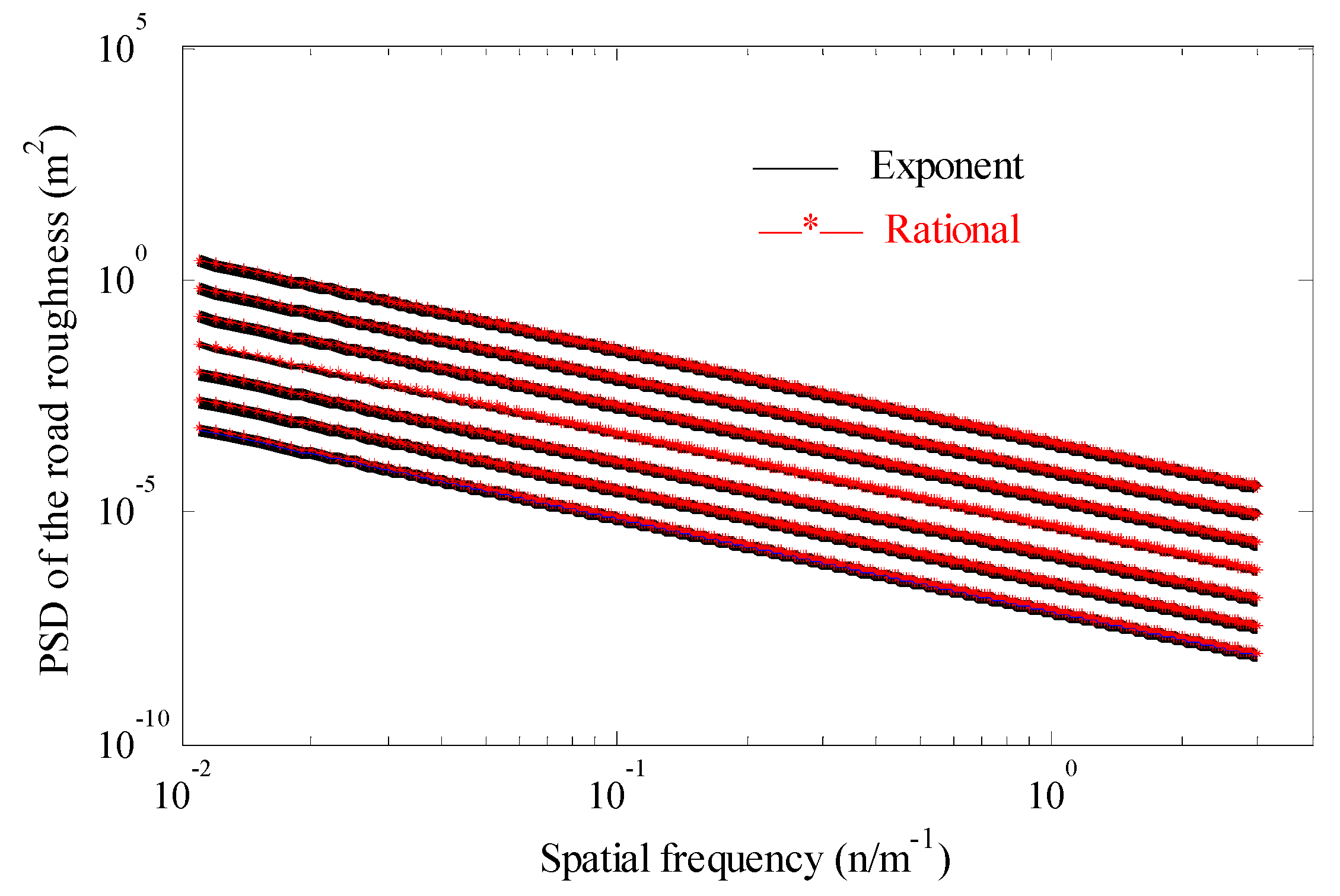
Considering values presented in [12], PSD of road roughness between rational white noise and ISO standard are compared using Equations (1)–(3). PDS road roughness results are shown in Figure 1.
It can be seen from Figure 1 that PSD of road roughness generated between rational white noise and ISO standard are consistent.

2.2. 3-D Road Roughness

2.2.1. Straight Driving Condition

One dimensional (1-D) autocorrelation function of the road roughness PSD based on white noise can be acquired using inverse Fourier transform [13]. 2-D auto-correlation function can be obtained by expanding the 1-D auto-correlation function and using isotropy of road roughness, as follows.
G q ( n 1 , n 2 ) = 4 π α ρ 2 [ α 2 + 4 π 2 ( n 1 2 + n 2 2 ) ] 3 / 2
where, n1 is spatial frequency with X-axis in m−1, n2 is spatial frequency with Y-axis in m−1 and G q ( n 1 , n 2 ) is PSD of 2-D road roughness with spatial frequency in m 3 .
According to [13], Fourier transform and PSD of 2-D road roughness can be expressed as Equations (7) and (8).
H ( f x , f y ) = lim l x , l y l x l x l y l y h ( x , y ) e j 2 π ( x f x + y f y ) d x d y
G ( f x , f y ) = lim l x , l y 1 4 l x l y | H ( f x , f y ) | 2
where, fx and fy are spatial frequencies with X-axis and Y-axis in m−1 respectively, lx and ly are surface road lengths; n2 is spatial frequency with Y-axis in m−1, h(x, y) is 3-D road roughness in m, G(fx, fy) is PSD of 2-D road roughness for spatial frequency in m3, and H(fx, fy) is Fourier transform of h(x, y).
Due to boundary of the actual road [10], Equations (7) and (8) can be expressed as Equations (9) and (10).
H ( f p , f q ) = Δ x Δ y m = 0 M 1 n = 0 N 1 h ( m Δ x , n Δ y ) e j 2 π ( p M m + q N n )
G ( f p , f q ) = Δ x Δ y M N | F ( f p , f q ) | 2
In addition,
f p = p M Δ x ;   p = 0 , 1 , 2 , , M 1
f q = q N Δ x ;   q = 0 , 1 , 2 , , N 1
where, M and N are sampling numbers, Δx and Δy are sample intervals, fp and fq are discrete spatial frequencies in m−1 and F(fp, fq) is Fourier transform of h(mΔx, nΔy).
With assumption of stationary random process, road defined in Equation (12) can be computed according to Equation (10) as follows.
F ( f p , f q ) = | F ( f p , f q ) | e φ ( f p , f q )
where ϕ (f, f) is phase angle of F(fp, fq).
Based on properties of 2-D Fourier transform, function H (p, q), i.e., the Fourier transform of h (m, n), may be satisfied by Equation (13).
H ( 1 , N + 1 n ) = c o n j [ H ( 1 , n ) ] ;
H ( M + 1 n , 1 ) = c o n j [ H ( m , 1 ) ] ;
H ( M / 2 , N + 1 n ) = c o n j [ H ( M / 2 , n ) ] ;
H ( M + 1 m , N / 2 ) = c o n j [ H ( m , N / 2 ) ] ;
H ( M + 1 m , N + 1 n ) = c o n j [ H ( m , n ) ] ;
where conj represents the conjugate; m = 1, 2, .., M/2 − 1; n = 1, 2, …, N/2 − 1.
Based on the above analysis, 3-D road roughness can be expressed by Equation (14).
h ( m , n ) = 1 M N p = 1 M 1 q = 1 N 1 F ( f p , f q ) e j 2 π ( p M m + q N n )
Following the analysis presented above, 3-D road roughness for level ISO-A and ISO-C cases are obtained. For instance, analysis is carried out considering level ISO-A excitation (at a velocity of 80 km/h). Results are shown in Figure 2.

2.2.2. Steering Working Condition

Movement trace of the vehicle is typically not straight under various steering conditions. As a result, PSD of road roughness while steering should also satisfy its statistical features. Based on the work presented in [14], a triangular mesh method is used for analysis.
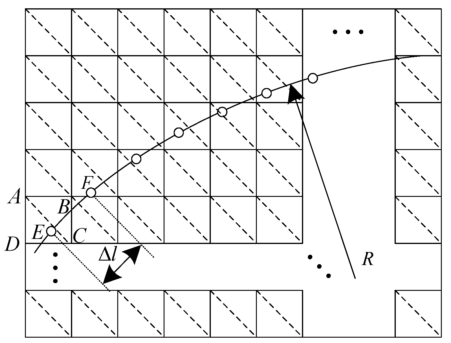
Road surface mode is considered to be a triangle grid space similar to the 3-D model shown in Figure 3. Adjacent points A, C, D and A, B, C in the 3-D model can form two triangular planes. When radius R and sampling interval Δl are known, coordinates of sampling point E can be located in the plane of triangle ACD. Then, road roughness at point E can be obtained by computing road roughness at points A, B, D. Following the procedure discussed above, road roughness of other points can be obtained as discussed in [14] and can be validated.

3. Rollover Index

A common method of defining rollover index (RI) is based on the difference in vertical tire loads between left and right sides of the vehicle [15].
RI = F z r F z l F z r + F z l ;   1 RI 1
where Fzl and Fzr are vertical tire forces on left and right side tires of the vehicle, respectively. When RI is equal to 1 or −1, right or left wheel lifts off.
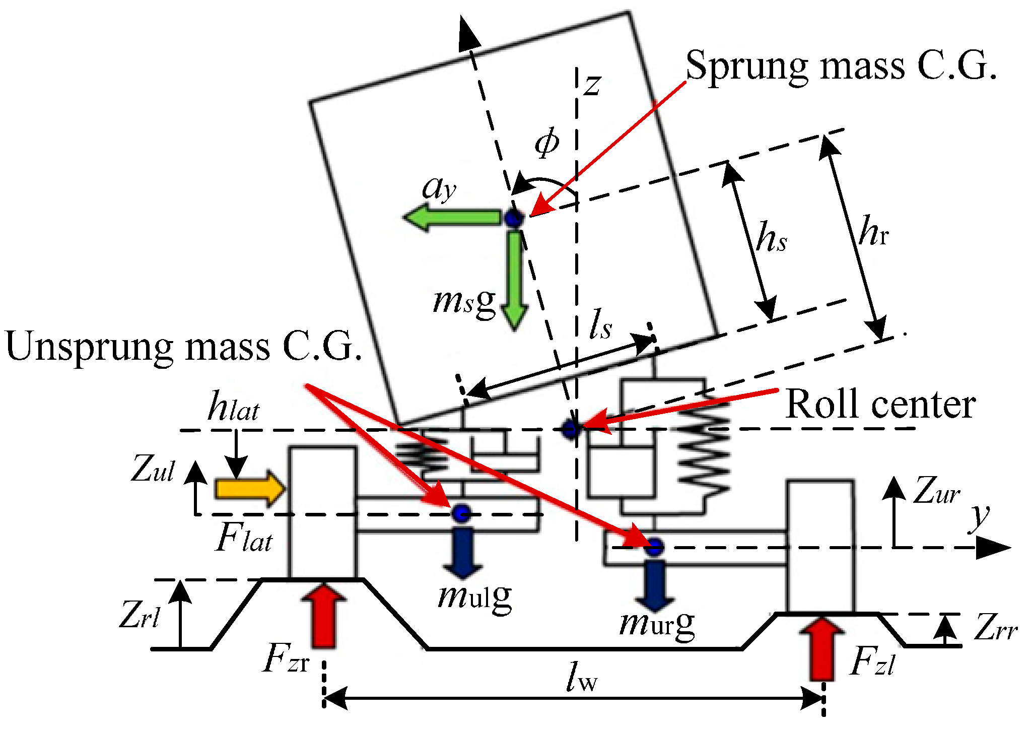
Forces on the tire Fzl and Fzr cannot be directly measured. To obtain RI in this situation, a 4-DOF vehicle model was developed as shown in Figure 4, A new RI* can be derived from Equation (15) [16].
RI * = F z r F z l F z r + F z l = l s l w k s l s sin ϕ + c l s ϕ ˙ cos ϕ + k s ( z u 1 z u 2 ) + c ( z ˙ u 1 z ˙ u 2 ) ( m g 2 k s z s 2 c z ˙ s + k s ( z u 1 + z u 2 ) + c ( z ˙ u 1 + z ˙ u 2 ) ) + 2 l w F l a t h l a t ( m g 2 k s z s 2 c z ˙ s + k s ( z u 1 + z u 2 ) + c ( z ˙ u 1 + z ˙ u 2 ) )
where hr is distance between C.G. height and roll center; φ represents roll angle; ay represents lateral acceleration; Flat is lateral force; hlat is distance from input lateral force to roll center; zrl and zrr are left and right road excitation, respectively. As shown in Figure 4, ls is body distance between left suspension and right suspension, i.e., ls is distance of a hinged between suspension and vehicle body; lw is track width; ks is suspension stiffness; zu1 and zu2 represent left and right unsprung mass positions, respectively; c is suspension damping; m is equal to sum of ms and mu, ms and mu are the sprung mass and unsprung mass of the vehicle, respectively.

4. Vehicle Dynamics Model

In this section, a half-car and a full-car dynamics models are utilized to analyze roll behavior of vehicle system.

4.1. Half-Car Dynamics Model

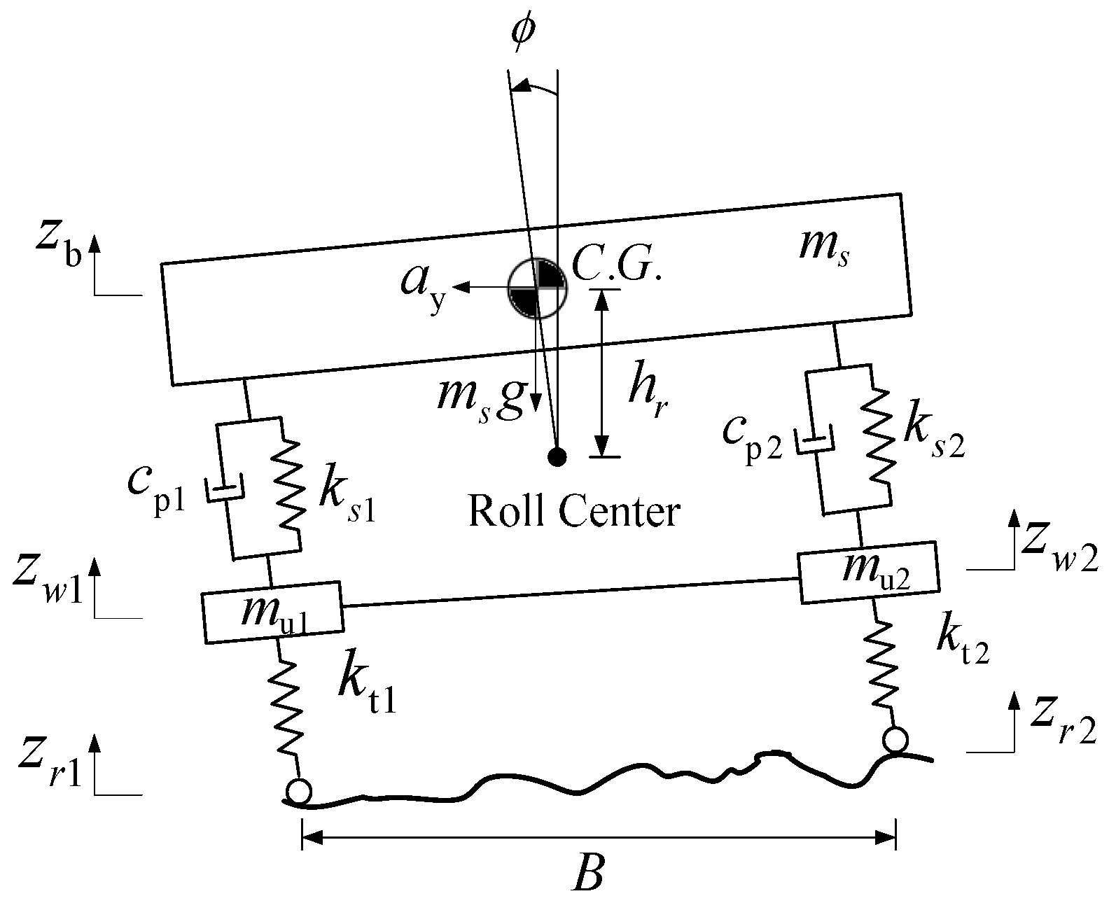
In practical scenarios, the real vehicle influence of wheel base or track on vehicle system can be neglected under some special conditions. In this study, the effect of the vehicle’s unsprung mass on roll dynamics is not neglected [15]. To obtain a functional relationship between road excitation and roll dynamics model, a half-car model is first presented, as shown in Figure 5. This model is a combination of a traditional 2-DOF bicycle model and a 4-DOF roll dynamics model used to describe yaw, lateral motion, and roll motion.
It should be noted that left and right steering angles in general would be approximately equal [17]. Symbols used in Figure 5 are listed in Table 2. Parameters in Table 2 are from the CARSIM® (E-Class, SUV). Here, lateral load transfer is considered for every wheel.
The half-car dynamics model is constructed based on the following assumptions [17,18].
  • Distance between two axles compared to turning radius was relative small, and steering wheel angle satisfies the following relationship: sinδf = δf, cosδf = 1.
  • Longitudinal effect of road profile was ignored.
  • There is no slip between the tires and road surface, and influence of ground longitudinal force on cornering characteristics of the tires was not considered.
  • The effect of the steering system was excluded, and front wheel angle was directly used as input.
  • The effect of air force was ignored.
  • Suspension elastic deformation steering and change of steering wheel alignment parameters were ignored.
  • The influence of bearing-free gap and lubricant membrane was ignored, and the bearing was taken as an equivalent spring–damper system in the vertical direction.

4.1.1. Tire Modelling

The Magic Formula (MF) Tire Model established by Pacejka [17] is utilized here. MF is a commonly used nonlinear tire model which has the general form shown below:
y = D sin [ C arctan { B x E ( B x arctan ( B x ) ) } ]
Y ( X ) = y ( x ) + S V x = X + S H
where X is input state, which represents slip ratio or slip angle; Y is output state and represents longitudinal force, lateral force or aligning torque. Factors C, D, B and E are usually derived from experiments. D is peak value of the curve; C determines shape of the obtained curve; B represents stiffness value of the curve; E represents curvature of the curve; SH and Sv are offset values of input and output states.
In combined slip conditions, lateral force will decrease due to longitudinal slip, and the longitudinal force will decrease due to lateral slip. Force and moments in this situation are obtained by multiplication of some weighing parameters with pure slip characteristics. However, tire longitudinal slip is defined to zero under constant vehicle longitudinal velocity. Various scaling factors are available in the MF model to check influence of changing tire properties without using real MF coefficients [18]. The details are stated in [17].
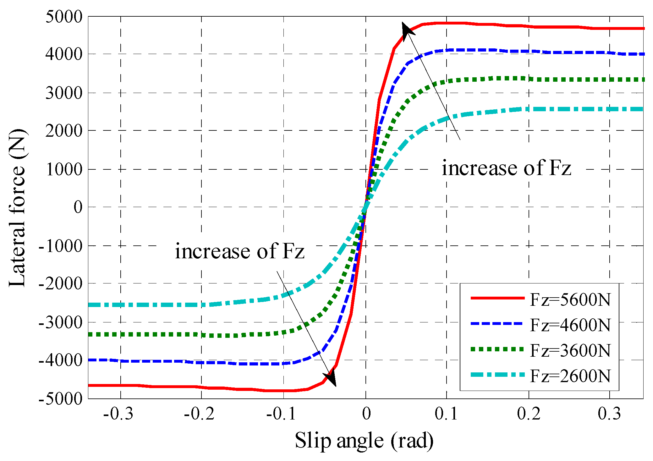
For known empirical formula, tire models for wheels of the vehicle can be obtained as shown in Figure 6.

4.1.2. Lateral Acceleration Calculation

Based on a traditional 2-DOF bicycle model [17], the dynamics equations can be expressed as follows:
M 1 a y m b h r ϕ ¨ ( F y f + F y r ) = 0 I z γ ˙ + I z x ϕ ¨ I x y ϕ ¨ 2 ( a F y f b F y r + M ) = 0
where Iz, Ixy and Izx are moment of inertia along Z axis, X-Y axis and Z-X axis, respectively. M is yaw moment, Fyf and Fyr represent lateral force of front wheel and rear wheel. Other parameters are shown in Table 2. More details are stated in [17,18].
To solve for the desired lateral acceleration, according to vehicle theory [17], front tire slip angle αf and rear tire slip angle αf can be calculated as follows:
{ α f = v y v x + a γ v x δ f α r = v y v x b γ v x
where vx and vy are longitudinal and lateral velocity, respectively. a and b are distance from C.G. to front axle and rear axle. δf is front steering angle. γ represents yaw rate.
In this paper, acceleration in Y-direction and yaw angle were obtained as follows:
v ˙ y = 2 ( C f + C r ) v y 2 ( a C f b C r ) γ M 1 v x + 2 C f δ f M 1 v x γ
γ ˙ = 2 ( a C f b C r ) v y 2 ( a 2 C f + b 2 C r ) γ I z v x + 2 a C f δ f I z
Desired lateral acceleration for a driver’s steering input is expressed as follows:
a y = v ˙ y + v x γ = 2 ( C f + C r ) v y 2 ( a C f b C r ) γ M 1 v x + 2 C f δ f M 1
Remark. 
Tire cornering stiffness is calculated using MF in Section 4.1.1, and other parameters can be obtained using CARSIM® simulation (version 8.02; Publisher: Mechanical Simulation Corporation, Detroit, MI, USA, 1996–2010).

4.1.3. 4-DOF Roll Dynamics Model

As shown in Figure 5, 4-DOF considered in this model are vertical translation of the sprung mass denoted by zb, roll motion of sprung mass denoted by φ and vertical translation of left and right unsprung mass denoted by zw1 and zw2, respectively.
Vertical force balance on sprung mass and two unsprung masses can be expressed as Equations (24)–(26).
m s z ¨ b = F s 1 + F s 2
m u 1 z ¨ w 1 = F s 1 k t 1 ( z w 1 z r 1 )
m u 2 z ¨ w 2 = F s 2 k t 2 ( z w 2 z r 2 )
where Fs1 and Fs2 are forces on both sides (left and right) of the suspension.
Roll dynamics of sprung mass are developed as follows.
( I x + m s h r ) ϕ ¨ = m s ( a y cos ϕ + g sin ϕ ) h r + B 2 ( F s 1 F s 2 )
where Ix is moment of inertia along X axis; ay is lateral acceleration; g is gravitational acceleration; Calculation is shown in Section 4.1.2.
Dynamics suspension forces are given in Equations (28) and (29).
F s 1 = k s 1 ( z b z w 1 B sin ϕ 2 ) c p 1 ( z ˙ b z ˙ w 1 B ϕ ˙ cos ϕ 2 )
F s 2 = k s 2 ( z b z w 2 + B sin ϕ 2 ) c p 2 ( z ˙ b z ˙ w 2 + B ϕ ˙ cos ϕ 2 )
Dynamics tire forces are given by Equations (30) and (31).
F t l = k t 1 ( z w 1 z r 1 )
F t r = k t 2 ( z w 2 z r 2 )
where Ftl and Ftr are forces on left and right sides of the tire, respectively.
Assuming cp1 = cp2 = cp and ks1 = ks2 = ks, and substituting Equations (28) and (29) into Equation (27), overall equations of motion are obtained as follows.
m s z ¨ s = k s 2 ( z b z w 2 + B sin ϕ 2 ) c p 2 ( z ˙ b z ˙ w 2 + B ϕ ˙ cos ϕ 2 ) k s 1 ( z b z w 2 B sin ϕ 2 ) c p 1 ( z ˙ b z ˙ w 1 B ϕ ˙ cos ϕ 2 )
m w 1 z ¨ w 1 = k s 1 ( z b z w 2 B sin ϕ 2 ) + c p 1 ( z ˙ b z ˙ w 1 B ϕ ˙ cos ϕ 2 ) k t 1 ( z w 1 z r 1 )
m w 2 z ¨ w 2 = k s 2 ( z b z w 2 + B sin ϕ 2 ) c p 2 ( z ˙ b z ˙ w 2 + B ϕ ˙ cos ϕ 2 ) k t 2 ( z w 2 z r 2 )
( I x + m s h R ) ϕ ¨ = m s ( a y cos ϕ + g sin ϕ ) h R k s B 2 2 sin ϕ c p B 2 2 ϕ ˙ cos ϕ   + k s B 2 ( z w z r ) + c p B 2 ( z ˙ w z ˙ r )
where z ¨ u 1 and z ¨ u 2 are acceleration on left and right sides of the suspension, respectively; z ˙ w z ˙ r is rattle space velocity between velocities of unsprung mass and road profile height.
Total tire forces on the ground include both static forces due to weight and dynamic force. Including both static and dynamic forces, total tire forces on the ground are given by
F z l = m s 2 g + m u 1 g k t 1 ( z w 1 z r 1 )
F z r = m s 2 g + m u 2 g k t 2 ( z w 2 z r 2 )
Since vertical forces Fzl and Fzr are equal to vertical forces on the tire, i.e., Ftl and Ftr, Equation (16) can also be expressed as follows.
RI h a l f = m u 2 z ¨ w 2 + F s 2 + m u 2 g m u 1 z ¨ w 1 F s 1 m u 1 g m u 2 z ¨ w 2 + F s 2 + m u 2 g + m u 1 z ¨ w 1 + F s 1 + m u 1 g
Considering mu1 = mu2 = mu, Equation (34) can be further simplified. By substituting Equations (31)–(34) into Equation (38), simplified RIhalf equation can be obtained as follows [16].
RI h a l f = m u ( z ¨ w 2 z ¨ w 1 ) 2 B 2 ( I x + m s h r 2 ) ( z ¨ b 1 z ¨ b 2 ) m u ( z ¨ w 2 + z ¨ w 1 ) + m s z ¨ b + ( 2 m u + m s ) g + 2 B 2 m s a y h r cos ϕ + 2 B 2 m s g h r sin ϕ m u ( z ¨ w 2 + z ¨ w 1 ) + m s z ¨ b + ( 2 m u + m s ) g
In addition,
z ¨ b 1 = z ¨ b cos ϕ B 2 ϕ ¨ + a y sin ϕ + g cos ϕ
z ¨ b 2 = z ¨ b cos ϕ + B 2 ϕ ¨ + a y sin ϕ + g cos ϕ
where, z ¨ b 1 represents acceleration of left suspension stiff body points attached to the vehicle body, z ¨ b 2 represents acceleration of right suspension stiff body points attached to the vehicle body, ( z ¨ b 1 z ¨ b 2 ) is difference sprung mass acceleration.

4.2. Full-Car Dynamics Model

Due to the complexity and uncertainty of practical vehicle driving and road conditions, front and rear coherence properties of vehicle and road can not be ignored. Steering wheel angle does not satisfy following relationship when compared with sharp turning: sinδfl = δfl, cosδfl = 1.
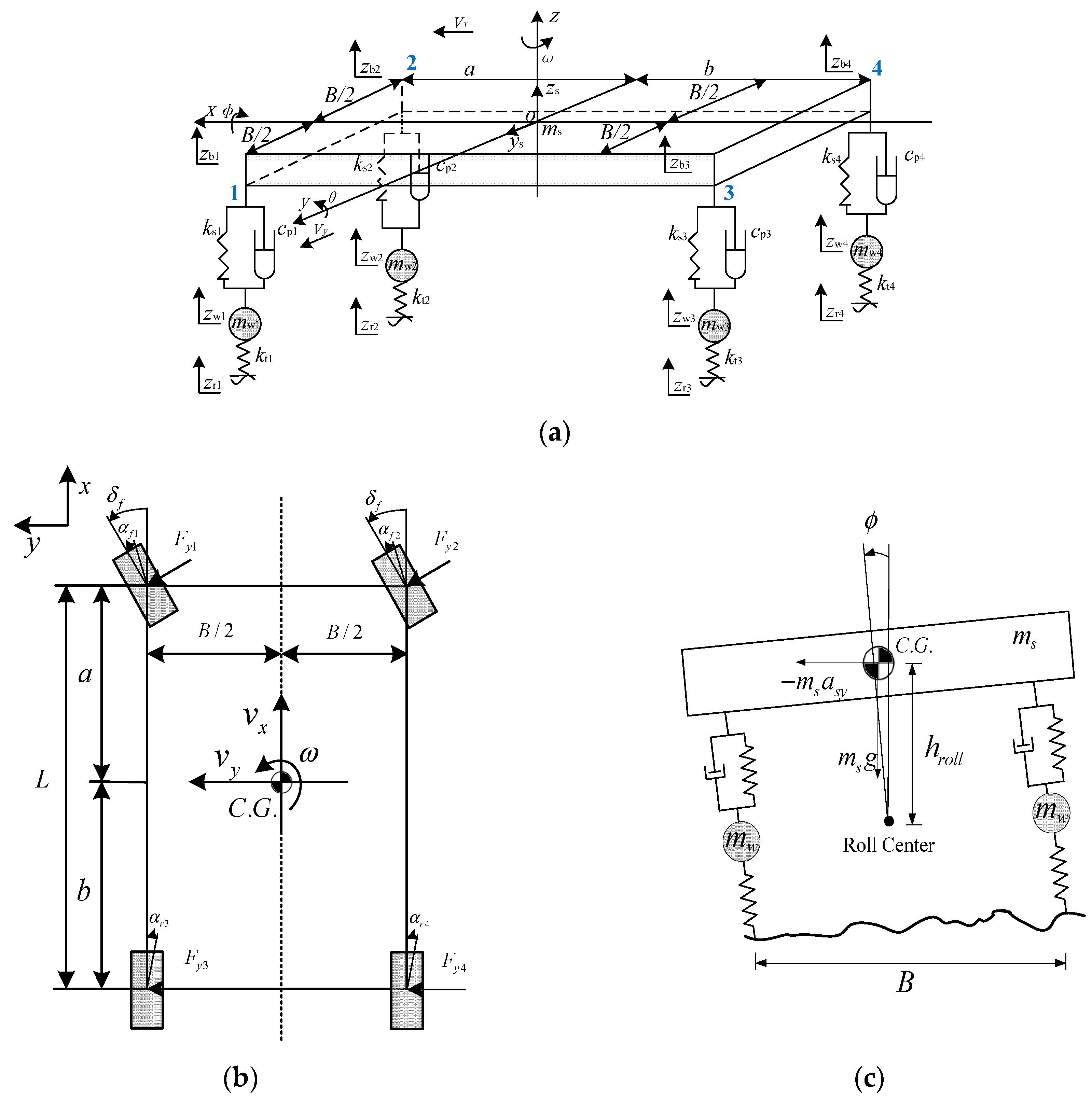
To further adapt vehicle driving and road conditions, compared to a 6-DOF half-car model, a full-car dynamics model with 9-DOF was developed based on the above assumptions [17,18]. Vertical and lateral coupling dynamics of the vehicle were considered simultaneously as shown in Figure 7. The 9-DOF included three degrees of freedom for vertical, pitch, and roll movement of the vehicle body, 4-DOF for vertical movement of unsprung masses, and 2-DOF for lateral and yawing movement of the vehicle. Descriptions of the symbols used in Figure 7 are listed in Table 3. Parameters in Table 3 also come from CARSIM® (E-Class, SUV; version 8.02; Publisher: Mechanical Simulation Corporation, Detroit, MI, USA, 1996–2010).

4.2.1. Kinematics of Vehicle System

In this section, the major coordinate system is established, i.e., SG is the earth-fixed inertial reference coordinate frame and Sv is the vehicle fixed non-inertial reference coordinate frame. Rotating angular velocity of Sv is wv, and Translating velocity of Sv is vv. The corresponding equations of the 9-DOF model are stated as follows. More details can be found in [15,17].

Translation of Sprung Mass C.G.

Position of C.G. of sprung mass in the reference coordinate frame Sv can be expressed as:
l o s = R y ( θ ) R x ( ϕ ) [ 0 0 h r o l l ] + [ 0 0 z b ] = [ h r o l l cos ϕ sin θ h r o l l sin θ h r o l l cos ϕ sin θ + z b ]
And,
R y ( θ ) = [ cos θ 0 sin θ 0 1 0 sin θ 0 c o s θ ] ;   R x ( ϕ ) = [ 1 0 0 0 cos ϕ sin ϕ 0 sin ϕ cos ϕ ]
Then,
( d d t ) G l o s = ( d d t ) v l o s + w v × l o s
where ‘×’ represents the cross-product operator, and wv = [0 0 w]T.
Velocity of sprung mass C.G. with respect to SG is denoted as the sum of translational vv of the vehicle reference coordinate frame Sv and the time derivative of position l o s .
v s = v v + ( d d t ) G = v v + ( d d t ) v l o s + w v × l o s = v v + l ˙ o s + w v × l o s
where “×” represents the cross-product operator, and vv = [Vx Vy 0]T.
The acceleration of sprung mass C.G. with respect to SG is calculated as:
a s = ( d d t ) G v s = + ( d d t ) v v v + w v × v v = v ˙ v + w v × v v

Translation of Unsprung Mass C.G.

As mentioned in Section 4.2.1, position of unsprung mass C.G. in the reference coordinate frame Sv can be expressed as:
l w 1 = [ a B 2 z w 1 h w 1 ] ;   l w 2 = [ a B 2 z w 2 h w 2 ] ; l w 3 = [ b B 2 z w 3 h w 3 ] ;   l w 4 = [ b B 2 z w 4 h w 4 ]
where, we denote that 1 as left-front of vehicle, 2 as right-front of vehicle, 3 as left-rear of vehicle and 4 as right-rear of vehicle. Also, hwi represents height of the roll axis above the ground for i = 1, 2, 3, 4.
Then, corresponding velocities and accelerations of vehicle unsprung mass C.G. with respect to SG, vsi and asi, i = 1, 2, 3, 4, can be calculated using Equations (45) and (46).

Rotations of C.G. of Unsprung Mass

Angular momentum Ds of the sprung mass can be expressed as:
D s = m s l o s l o s × v s + I s w s = ( D C G ) s + ( D w ) s
where, (DCG)s is angular momentum of sprung mass C.G. due to motion, (Dw)s is angular momentum of sprung mass C.G. due to rotation, and w s = [ ϕ ˙   θ ˙   w ] T .
Also, angular momentum Dw of unsprung mass can be expressed as:
D w = i = 4 4 [ m w i ( w i × v i ) + I w i w v ]
Total angular momentum D of vehicle can be expressed as:
D = D s + D w

4.2.2. Dynamics of Vehicle System

Based on Newton’s law, dynamics equations of the 9-DOF full-car model are as follows.
  • Equation (51) for vehicle body vertical motion
    i = 1 4 F s i = m s z ¨ s
    where Fsi is suspension force. Corresponding equations can be obtained as follows.
    F s 1 = k s 1 ( z b 1 z w 1 ) c p 1 ( z ˙ b 1 z ˙ w 1 ) ; F s 2 = k s 2 ( z b 2 z w 2 ) c p 2 ( z ˙ b 2 z ˙ w 2 ) ; F s 3 = k s 3 ( z b 3 z w 3 ) c p 3 ( z ˙ b 3 z ˙ w 3 ) ; F s 4 = k s 4 ( z b 4 z w 4 ) c p 4 ( z ˙ b 4 z ˙ w 4 ) ;
    And,
    z b 1 = z b + B 2 sin ϕ a sin θ ; z b 2 = z b B 2 sin ϕ a sin θ ; z b 3 = z b + B 2 sin ϕ + b sin θ ; z b 4 = z b B 2 sin ϕ + b sin θ ;
  • Equation (54) for unsprung mass vertical motion
    m w 1 z ¨ w 1 = k s 1 ( z w 1 z b 1 ) c p 1 ( z ˙ w 1 z ˙ b 1 ) k t 1 ( z w 1 z r 1 ) ; m w 2 z ¨ w 2 = k s 2 ( z w 2 z b 2 ) c p 2 ( z ˙ w 2 z ˙ b 2 ) k t 2 ( z w 2 z r 2 ) ; m w 3 z ¨ w 3 = k s 3 ( z w 3 z b 3 ) c p 3 ( z ˙ w 3 z ˙ b 3 ) k t 3 ( z w 3 z r 3 ) ; m w 4 z ¨ w 4 = k s 4 ( z w 4 z b 4 ) c p 4 ( z ˙ w 4 z ˙ b 4 ) k t 4 ( z w 4 z r 4 ) ;
  • Equation (55) for vehicle body pitch motion
    i = 1 4 M y i = I y i θ ¨ = ( F s 1 + F s 2 ) a ( F s 3 + F s 4 ) b + m s g h r o l l sin θ
    where Myi, i = 1, 2, 3, 4 is vehicle roll moment.
  • Equation (56) for vehicle body roll motion
    i = 1 4 M x i = I x ϕ ¨ = ( F s 2 + F s 4 ) B 2 ( F s 1 + F s 3 ) B 2 + m s h r o l l ( g sin θ + a s y )
    where Mxi, i = 1, 2, 3, 4 is vehicle roll moment.
  • Equation (57) for vehicle lateral motion
    i = 1 4 F y i = m s a s y + i = 1 4 m w i a w y i = ( F y 1 + F y 2 ) cos δ f + ( F y 3 + F y 4 ) cos δ r ;
    where Fyi, i = 1, 2, 3, 4, is tire lateral force.
  • Equation (58) for the vehicle yaw motion
    M = I z ω ˙ = b ( F y 3 + F y 4 ) cos δ r a ( F y 1 + F y 2 ) cos δ f B 2 ( F y 2 F y 1 ) sin δ r B 2 ( F y 4 + F y 3 ) sin δ f + M z 1 + M z 2 + M z 3 + M z 4
    where Mzi, i = 1, 2, 3, 4 is tire self-aligning moment.
Thus, Equation (59) can be expressed as follows.
RI f u l l = m u 3 z ¨ w 3 + F s 3 + m u 3 g + m u 4 z ¨ w 4 + F s 4 + m u 4 g m u 1 z ¨ w 1 F s 1 m u 1 g m u 2 z ¨ w 2 F s 2 m u 2 g m u 3 z ¨ w 3 + F s 3 + m u 3 g + m u 4 z ¨ w 4 + F s 4 + m u 4 g m u 1 z ¨ w 1 F s 1 m u 1 g m u 2 z ¨ w 2 F s 2 m u 2 g

5. Simulation and Validation

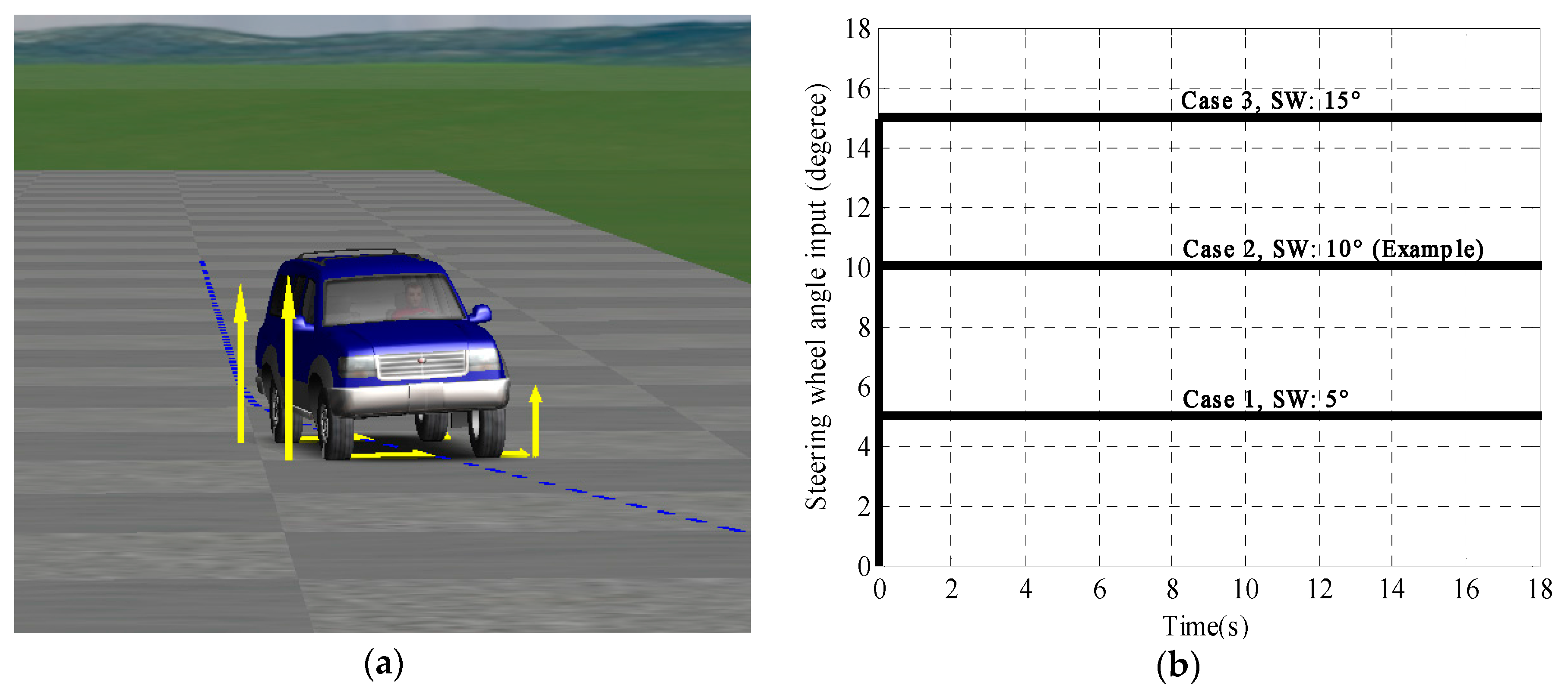
To validate the two proposed models, an industrial standard vehicle dynamics simulation software, CARSIM® was used to carry out simulations [16,19,20]. A standard SUV model was chosen from CARSIM® vehicle models as shown in Figure 8. Simulation and validation results of vehicle roll behavior were carried out under steering wheel (SW) input 10° condition as an example case to facilitate better analysis of vehicle roll behavior.
Based on the above analysis, half-car and full-car models proposed in Section 4 were simulated in MATLAB to study performance of vehicle roll behavior with or without road excitation (two representatives). It is assumed that the tire does not loose ground contact. Here, the J-turn maneuver [15] was utilized to illustrate roll behavior for steering wheel at 10° at a velocity of 80 km/h with presence of road excitation. It was concluded from the results vehicle roll behavior mainly depends on roll angle, roll rate, and yaw rate. It should be noted that roll angle is variable under varying steering wheel input, and roll angle can be seen as a reference validation for vehicle roll behavior.

5.1. Roll Behavior without Road Excitation

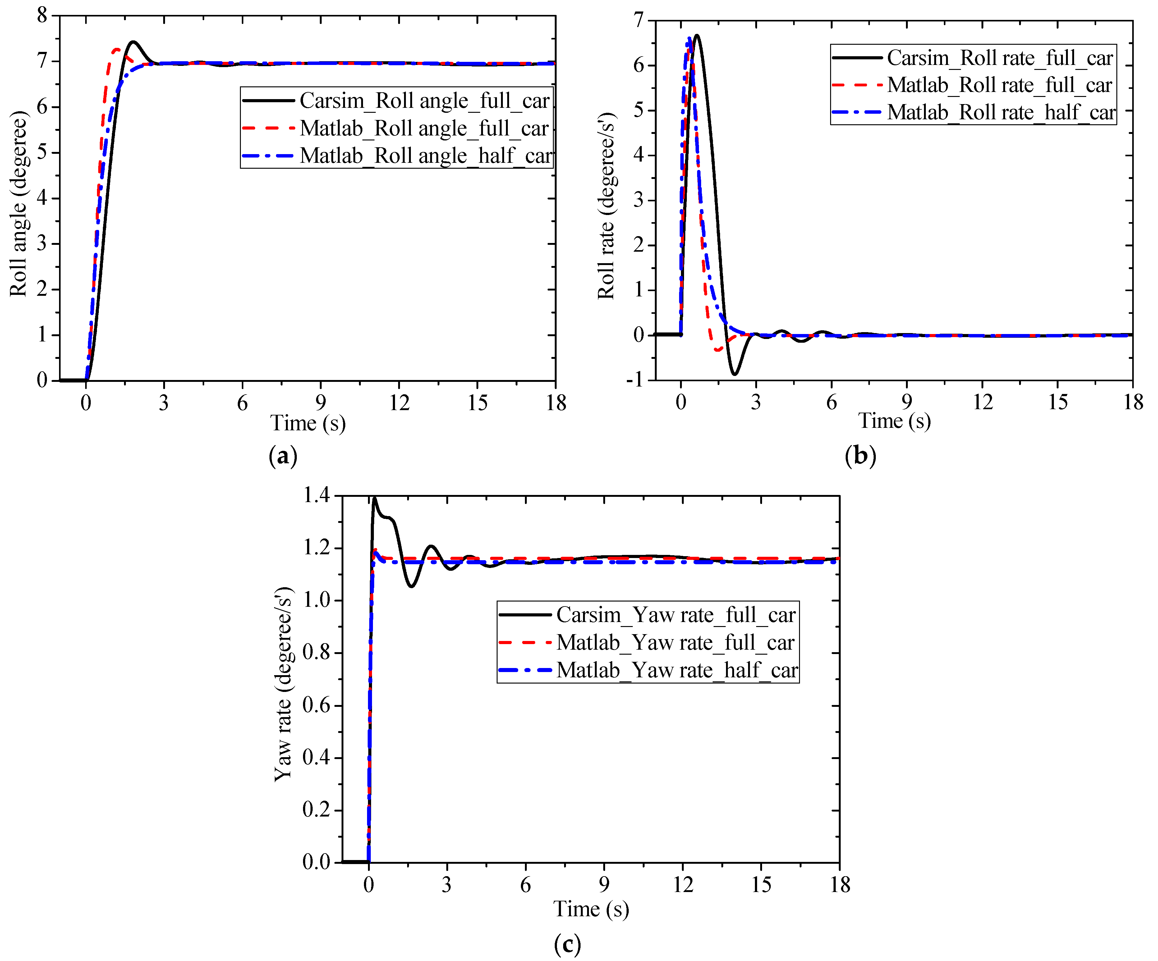
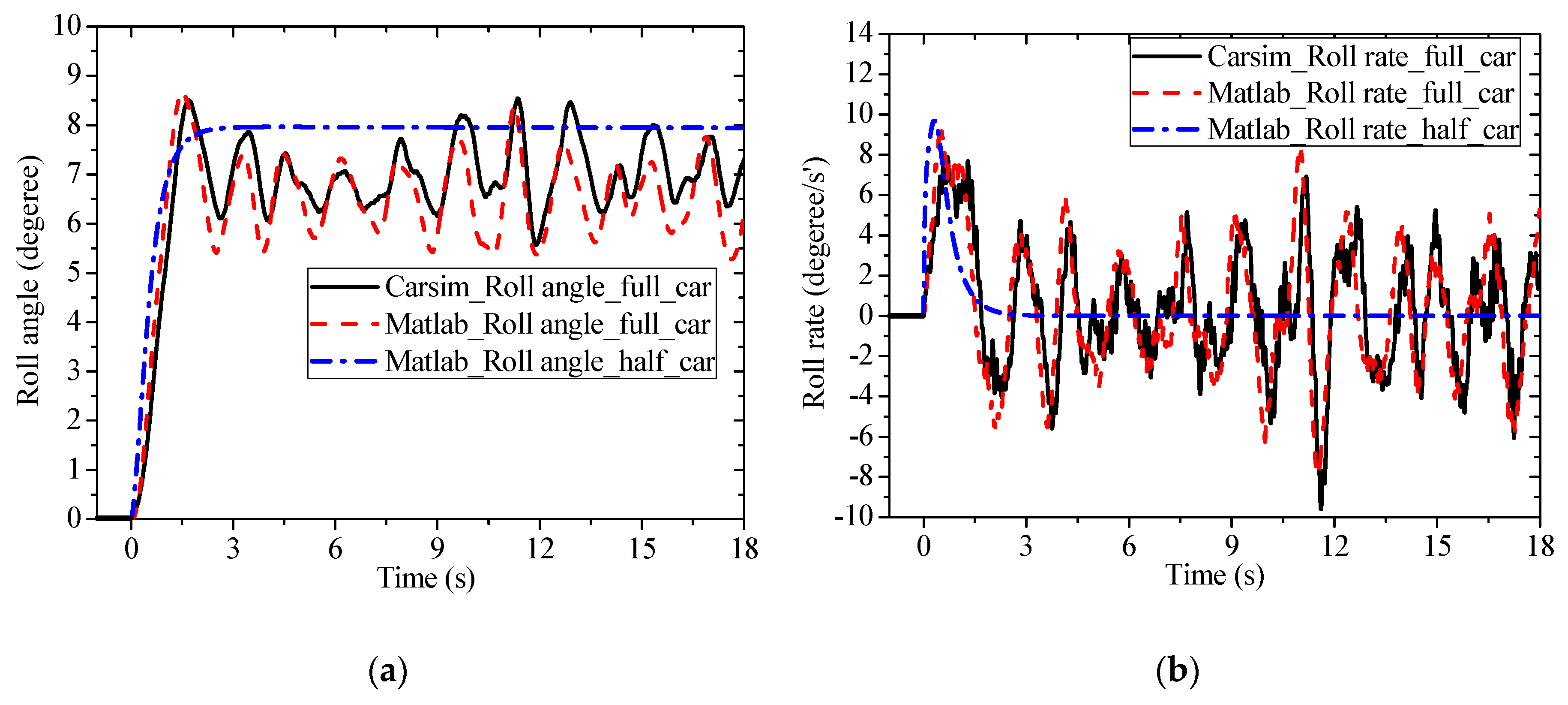
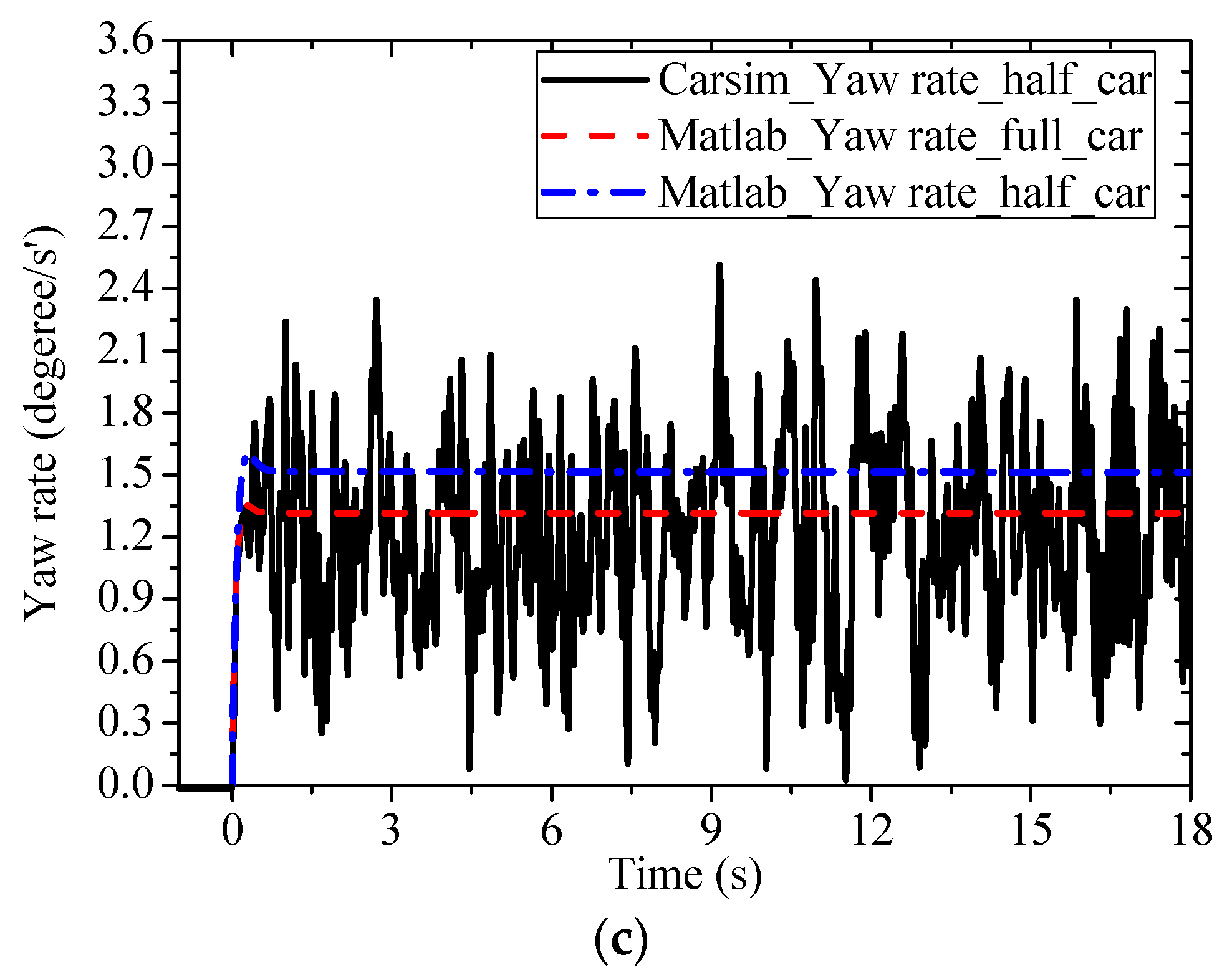
Here, using vehicle dynamics model from Section 4, performance of vehicle roll behavior is simulated without presence of road input. Initial conditions used in the simulation are listed in Table 1 and Table 2. Corresponding performance of roll behavior result parameters are shown in Figure 9. It can be seen from Figure 9 that without road excitation, half-car and full-car model are approximately equivalent. The E-Class (SUV) level car model in CARSIM® was used as benchmark results. Calculations carried out in MATLAB were found to be consistent with the CARSIM data. This suggests that vehicle dynamics model presented in Section 4 can be considered accurate to depict system dynamics under this condition.

5.2. Considering Road Excitation

Case1: Level ISO-A road excitation

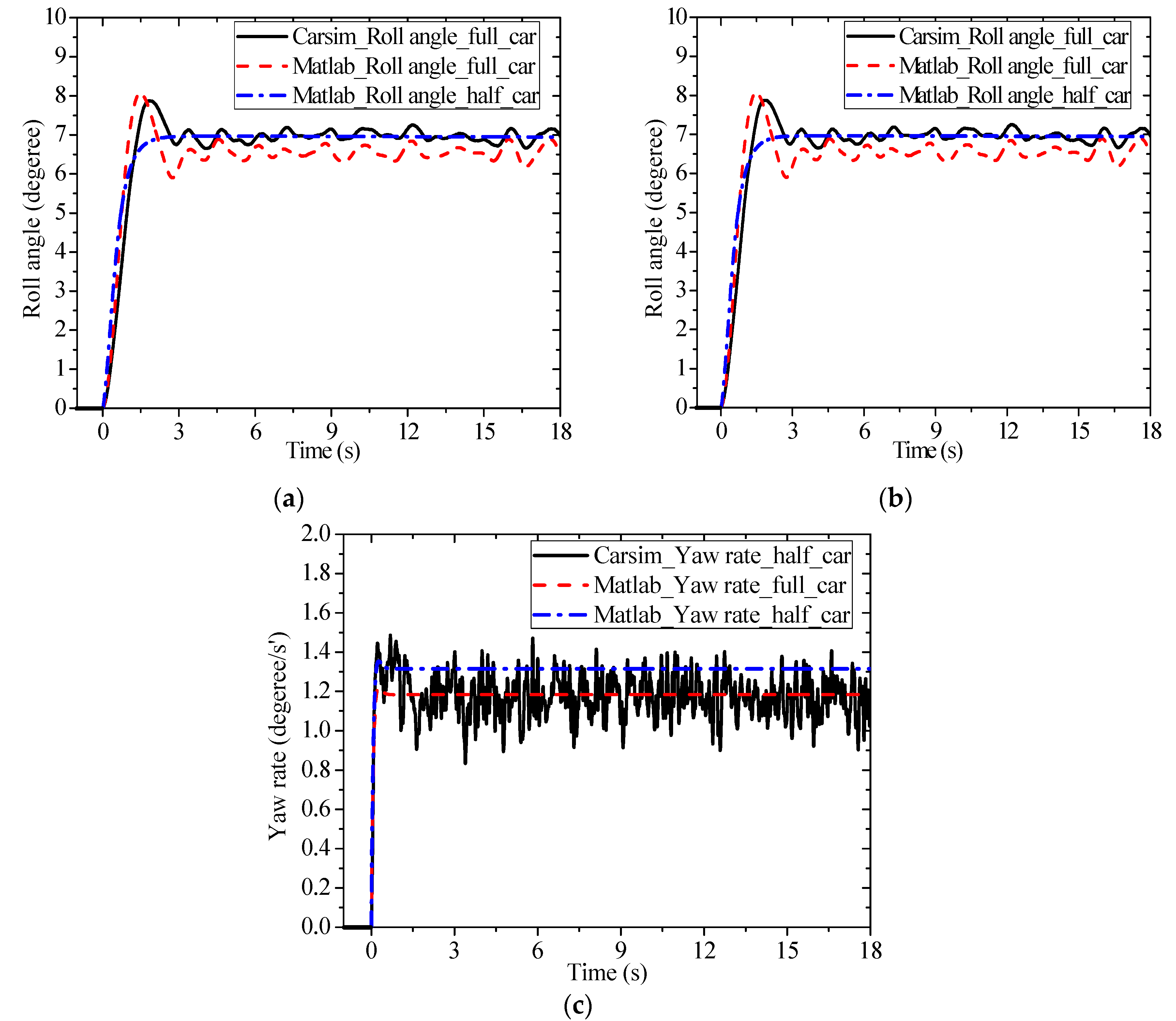
Based on the vehicle dynamics model presented in Section 4, performance of vehicle roll behavior was also computed considering level ISO-A road excitation. Roll angle, roll rate, and yaw rate for roll behavior are shown in Figure 10. From the results, it can be seen that with road excitation, vehicle roll responses are different under level ISO-A road excitation. With E-Class (SUV) level car model in CARSIM® as a benchmark, simulation data of 9-DOF full-car model was found to be consistent with CARSIM data, i.e., half-car roll model and full-car roll model are no more equivalent.

Case 2: Level ISO-C road excitation

For level ISO-C road excitation case, roll angle, roll rate, and yaw rate for roll behavior are shown in Figure 11. It can be seen from the results that vehicle response for different dynamics models have significant impact on roll behavior under level ISO-C road excitation, and influence of road excitation cannot be ignored in this situation [21,22,23,24,25,26,27].
To further illustrate difference between 6-DOF and 9-DOF models with road excitation and various steering wheel inputs, vehicle responses were statistically analyzed. Previous research divided statistical parameters into dimensional parameters and non-dimensional parameters [21]. Dimensional parameters such as mean value, variance, maximum, etc., are used to depict steady stochastic processes especially suitable for statistical process description. Non-dimensional parameters, including Kurtosis, Crest factor, Clearance factor, etc., are utilized to describe transient processes, especially suitable for non-statistical process description. Vehicle steering wheel input is a transient response; due to this non-dimensional parameters should be adopted to study vehicle responses. Five widely applied features that suitable for depicting these temporary characteristics as listed in Table 4 [22,23]. Parameter F1 and F4 may indicate distribution characteristics. Parameters F2~F3, F5 represent influence of impact or impulse input.
To illustrate error in different dynamics models, with E-Class (SUV) level car model in CARSIM® as a benchmark, accuracy of proposed models and comparison results are summarized in Table 5 and Table 6.
Table 5 and Table 6 show that different dynamics models have significant impact on the calculation accuracy, and higher accuracy using 9-DOF model can be obtained when coupling relationships exists between road excitation and vehicle dynamics.

5.3. Disscussion

From results in Figure 6, it can be seen that under identical vertical loads, when slip angle was smaller than 0.08 rad, lateral force on front rear tires increases linearly with increase in slip angle. However, when slip angle was larger than 0.08 rad, rate of lateral force increment gradually slows down, and relationship with slip angle is no longer linear. In addition, for identical slip angles, a larger vertical load was accompanied by a larger lateral force. Thus, for the tire model, lateral force is a function of slip angle and vertical load. Relationships between slip angle and vertical load were nonlinear [18]. This leads to nonlinear behavior of tire lateral forces under various steering wheel inputs.
To further illustrate superiority of the proposed model, 5° and 15° steering wheel input situations were also simulated. Similar results were obtained without road excitation, i.e., 6-DOF half-car model and 9-DOF full-car model are approximately equivalent under these conditions. However, 6-DOF model and 9-DOF model have significant differences with road input. Corresponding simulation results for different steering wheel inputs and various road excitations are shown in Table 7, Table 8, Table 9 and Table 10, which are described as shown in Figure 12. In Figure 12a, feature F1, comparison of 6-DOF and 9-DOF models for road level ISO-A/C excitation is shown. It can be seen that accuracy of vehicle responses were higher under road level ISO-A excitation than road level ISO-C, i.e., higher road level lead to higher error. Roll angle and roll rate accuracy for vehicle responses of 6-DOF model was a maximum of 60% under road level ISO-A/C excitation. Roll angle and roll rate calculation accuracy for vehicle responses of 9-DOF model was 85% under road level ISO-A/C excitation. With increase of the steering wheel input, as in the case of F2, accuracy for 6-DOF model was a maximum of 58% under road level ISO-A/C excitation. However, for a 9-DOF model accuracy declined at a slower rate than 6-DOF model as shown in Figure 12b. From F3 perspective, an increase in road level resulted in accuracy for vehicle responses of 6-DOF and 9-DOF model to reach a maximum of 90% under road level ISO-A/C excitation. However, for a 6-DOF model accuracy declined at a faster rate than 9-DOF model as shown in Figure 12c. Further, from F4 and F5 perspectives, Figure 12d,e show that accuracy of 9-DOF model vehicle responses are higher under road level ISO-C excitation and steering wheel input 15° than 6-DOF model vehicle responses under road level ISO-A excitation and steering wheel input 5°.
Based on the above analysis, simulation results show that accuracy of statistical features calculation for 6-DOF model reached a maximum of 65% for all situations. Lower accuracy of statistical features follows increase in the angle of steering wheel input; accuracy of statistical features calculated for 9-DOF model was higher than 85%.
Comparison of simulation results from MATLAB and CARSIM® allows verification of the proposed 9-DOF full-car model for roll behavior with or without road excitation condition. A 6-DOF half-car model was found to be suitable in conditions without road excitation. Influence of vehicle model on roll behavior should be adopted for the full-car model while analyzing vehicle roll behaviors with large steering wheel input and considering road excitation.

6. Conclusions

In this paper, performance of vehicle roll behavior under various road excitation and steering wheel inputs was studied using 6-DOF half-car and 9-DOF full-car models. With the proposed method, influence of half-car and full-car models on vehicle roll behavior and coupling relationships between vehicle vertical and lateral response was comprehensively studied. The main conclusions are as follows:
  • Based on the generating theories, a 3-D road profile model was first developed with road level ISO-A/C as the half-car and full-car dynamics model input. State response of vehicle roll behavior relationships between road excitation and steering wheel input were calculated with half-car and full-car models. From the results, it was concluded that road excitation and steering wheel input have a significant influence on vehicle roll behaviors, i.e., 6-DOF model was suitable for small steering wheel input without road excitation. Average accuracy of this model was determined to be a maximum of 65%. A 9-DOF model was more accurate for large steering input with road excitation with an average accuracy higher than 85%.
  • Calculated vehicle response of vehicle roll behavior was validated using CARSIM®. Compared to calculation results, CARSIM® simulation results showed that proposed half-car model can provide a satisfying result without road excitation. However, full-car model can provide better description of system dynamics under various road excitation and large steering wheel input conditions to further validate the conclusions.
In the future, the proposed model will be applied to an actual road profile and a practical full-car will be realized using the proposed 9 DOF full-car model. In addition, our research will extend to state estimation and control of a full-car nonlinear suspension system and focus on application of these results for improving vehicle performance, especially on the aspects of ride comfort and road handling.
Acknowledgments

This work was supported by the National Natural Science Foundation of China (Grant No. U1564210), Innovative Talent Support Program for Post-Doctorate of China (Grant No. BX201600017) and China Postdoctoral Science Foundation (Grant No. 2016M600934).

Author Contributions

Zhen-Feng Wang and Ye-Chen Qin conceived and designed the simulations; Zhen-Feng Wang wrote the paper and analyzed the data; and Ye-Chen Qin, Liang Gu, Ming-Ming Dong, Jagat-Jyoti Rath and Bin Bai provided some suggestions and revised the paper.

Conflicts of Interest

The authors declare no conflict of interest.

References

  1. Whitehead, R.; Travis, W.; Bevly, M.D.; Flowers, G. A Study of the Effect of Various Vehicle Properties on Rollover Propensity; SAE Technical Paper; SAE International: Detroit, MI, USA, 2004. [Google Scholar]
  2. Yim, S. Design of a preview controller for vehicle rollover prevention. IEEE Trans. Veh. Technol. 2011, 60, 4217–4226. [Google Scholar] [CrossRef]
  3. Yi, K.Y.; Yoon, J.Y.; Kim, D.S. Model-based estimation of vehicle roll state for detection of impending vehicle rollover. In Proceedings of the 2007 American Control Conference, New York, NY, USA, 9–13 July 2007; Volume 1, pp. 1624–1629. [Google Scholar]
  4. Rajamani, R.; Piyabongkan, D.; Tsourapas, V.; Lew, J.Y. Real-time estimation of roll angle and CG hight for active rollover prevention applications. In Proceedings of the 2009 American Control Conference, St. Louis, MO, USA, 10–12 June 2009; Volume 1, pp. 433–435. [Google Scholar]
  5. Rajamani, R.; Piyabongkan, D.; Tsourapas, V.; Lew, J.Y. Parameter and state estimation in vehicle roll dynamics. IEEE Trans. Intell. Transp. Syst. 2011, 12, 1558–1567. [Google Scholar] [CrossRef]
  6. Chen, B.C.; Peng, H. Differential-Braking-Based rollover prevention for sport utility vehicles with human-in-the-loop evaluations. Veh. Syst. Dyn. 2001, 36, 359–389. [Google Scholar] [CrossRef]
  7. Larish, C.; Piyabongkan, D.; Tsourapas, V.; Rajamani, R. A new predictive lateral load transfer ratio for rollover prevention systems. IEEE Trans. Veh. Technol. 2013, 62, 2928–2936. [Google Scholar] [CrossRef]
  8. Imine, H.; Benallegue, A.; Madani, T.; Srairi, S. Rollover risk prediction of heavy vehicle using high-order sliding–mode observer: Experimental results. IEEE Trans. Veh. Technol. 2014, 63, 2533–3543. [Google Scholar] [CrossRef]
  9. Van der Westhuizen, S.F.; Els, P.S. Slow active suspension control for rollover prevention. J. Terramech. 2013, 50, 29–36. [Google Scholar] [CrossRef]
  10. ISO. Mechanical Vibration-Road Surface Profiles-Reporting of Measured Data; ISO 8601-1995; International Organization for Standardization: Geneva, Switzerland, 1995. [Google Scholar]
  11. Michelberger, P.; Palkovics, L.; Bokor, J. Robust design of active suspension system. Int. J. Veh. Des. 1993, 14, 145–165. [Google Scholar]
  12. Wu, Z.C.; Chen, S.Z.; Yang, L. Model of Road Roughness in Time Domain Based on Rational Function. Trans. Beijing Inst. Technol. 2009, 29, 795–798. [Google Scholar]
  13. Qin, Y.C.; Dong, M.M.; Langari, R.; Gu, L.; Guan, J.F. Adaptive hybrid control of vehicle semiactive suspension based on road profile estimation. Shock Vib. 2015, 2015. [Google Scholar] [CrossRef]
  14. Detweiler, Z.R.; Ferris, J.B. Interpolation methods for high-fidelity three-dimensional terrain surfaces. J. Terramech. 2011, 47, 209–217. [Google Scholar] [CrossRef]
  15. Rajamani, R. Vehicle Dynamics and Control, 2nd ed.; Springer: New York, NY, USA, 2012. [Google Scholar]
  16. Phanomchoeng, G.; Rajamani, R. New rollover index for the detection of tripped and untripped rollovers. IEEE Trans. Ind. Electron. 2013, 60, 4726–4737. [Google Scholar] [CrossRef]
  17. Pacejia, H.B. Tyre and Vehicle Dynamics; Butterworth-Heinemann: Oxford, UK, 2002. [Google Scholar]
  18. Tan, D.; Lu, C. The influence of the magnetic force generated by the in-wheel motor on the vertical and lateral coupling dynamics of electric vehicles. IEEE Trans. Veh. Technol. 2016, 65, 4655–4668. [Google Scholar] [CrossRef]
  19. Rath, J.J.; Defoort, M.; Karimi, H.R.; Veluvolu, K.C. Output feed-back active suspension control with higher order terminal sliding mode. IEEE Trans. Ind. Electron. 2017, 64, 1392–1403. [Google Scholar] [CrossRef]
  20. Rath, J.J.; Defoort, M.; Veluvolu, K.C. Rollover index estimation in the presence of sensor faults, unknown inputs, and uncertainties. IEEE Trans. Intell. Transp. Syst. 2016, 17, 2949–2959. [Google Scholar] [CrossRef]
  21. Palla, A.; Gnecco, I.; Lanza, L.G. Non-dimensional design parameters and performance assessment of rainwater harvesting systems. J. Hydrol. 2011, 40, 65–76. [Google Scholar] [CrossRef]
  22. Qin, Y.C.; Dong, M.M.; Zhao, F.; Gu, L. Road profile classification for vehicle semi-active suspension system based on adaptive neuro-fuzzy inference system. In Proceedings of the 2015 54th IEEE Conference on Decision and Control, Osaka, Japan, 15–18 December 2015; Volume 1, pp. 1533–1538. [Google Scholar]
  23. Wang, Z.F.; Dong, M.M.; Qin, Y.C.; Du, Y.C.; Zhao, F.; Gu, L. Suspension system state estimation using adaptive Kalman filtering based on road classification. Veh. Syst. Dyn. 2016, 55, 371–398. [Google Scholar] [CrossRef]
  24. Qin, Y.C.; Xiang, C.L.; Wang, Z.F.; Dong, M.M. Road excitation classification for semi-active suspension system based on system response. J. Vib. Control 2017. [Google Scholar] [CrossRef]
  25. Zhao, F.; Ge, S.S.; Tu, F.W.; Qin, Y.C.; Dong, M.M. Adaptive neural network control for active suspension system with actuator saturation. IET Control Theory Appl. 2016, 14, 1696–1705. [Google Scholar] [CrossRef]
  26. Qin, Y.C.; Zhao, F.; Wang, Z.F.; Gu, L.; Dong, M.M. Comprehensive analysis influence of controllable damper time delay on semi-active suspension control strategies. J. Vib. Acoust. 2017. [Google Scholar] [CrossRef]
  27. Wang, Z.F.; Dong, M.M.; Zhao, W.P.; Gu, L. A novel tread model for tire modelling using experimental modal parameters. J. Vibroeng. 2017, 19, 1225–1240. [Google Scholar] [CrossRef]
Figure 1. Results of parameters estimation.
Applsci 07 00570 g001
Figure 2. 3-D road roughness for Level ISO-A (at a velocity of 80 km/h).
Applsci 07 00570 g002
Figure 3. Sampling of elevation about steering track road roughness.
Applsci 07 00570 g003
Figure 4. Roll behavior of vehicle system.
Applsci 07 00570 g004
Figure 5. Half-car roll dynamics model.
Applsci 07 00570 g005
Figure 6. Influence of vertical force on tire lateral force.
Applsci 07 00570 g006
Figure 7. 9-DOF vehicle dynamics model. (a) Full-car dynamics model. (b) Lateral dynamics model. (c) Roll dynamics model.
Applsci 07 00570 g007
Figure 8. CARSIM simulation of roll behavior under various road excitation conditions. (a) Animation Screen. (b) Steering wheel input.
Applsci 07 00570 g008
Figure 9. Results without road excitation (steering wheel angle was 10° at 80 km/h). (a) Roll angle; (b) Roll rate; (c) Yaw rate.
Applsci 07 00570 g009
Figure 10. Results with road Level ISO-A excitation (steering wheel angle was 10° at 80 km/h). (a) Roll angle; (b) Roll rate; (c) Yaw rate.
Applsci 07 00570 g010
Figure 11. Results with road Level ISO-C excitation (steering wheel angle was 10° at 80 km/h). (a) Roll angle, (b) Roll rate, (c) Yaw rate.
Applsci 07 00570 g011aApplsci 07 00570 g011b
Figure 12. Accuracy of statistical features for vehicle state calculations using 6-DOF and 9-DOF models under road Level ISO-A/C excitation and steering wheel 5°, 10° and 15° conditions. (a) Kurtosis, (b) Crest factor, (c) Clearance factor, (d) Shape factor, (e) Impulse factor.
Applsci 07 00570 g012
Table 1. Estimated results of road parameters.
Road Levelα/(m−1)ρ/mGq(n0)
A0.00110.015316
B0.030664
C0.0611256
D0.12221024
E0.24444096
F0.488816,384
G0.977665,536
H1.955226,2144
Table 2. Description of symbols for 6-DOF half-car dynamics model.
Vehicle Model ParametersSymbolUnit
Lateral accelerationaym/s2
Roll angle of sprung massφdeg (°)
Front tire cornering stiffnessCfN/°
Rear tire cornering stiffnessCrN/°
Total mass of the vehicleM1kg
Sprung mass of vehicle bodymskg
Unsprung mass of vehicle left sidemu1kg
Unsprung mass of vehicle right sidemu2kg
Suspension stiffness of left sideks1N/m
Suspension stiffness of right sideks2N/m
Suspension damping coefficient of left sidecp1Ns/m
Suspension damping coefficient of right sidecp2Ns/m
Tire stiffness of left sidekt1N/m
Tire stiffness of right sidekt2N/m
Sprung mass displacement of vehicle bodyzbm
Unsprung mass displacement of left sidezw1m
Unsprung mass displacement of right sidezw2m
Road profile of left sidezr1m
Road profile of right sidezr2m
Track widthBm
Distance between roll center to C.G. of sprung masshrm
Roll damping coefficientCrollNs/m
Roll stiffness coefficientKrollN/m
Table 3. Description of symbols used for 9-DOF full-car dynamics model.
Vehicle Model ParametersSymbolUnit
Steering angle of front left sideδfldeg (°)
Steering angle of front right sideδfrdeg (°)
Rear tire slip angleαrdeg (°)
Displacement of the front/rear axleBm
Longitudinal displacement of chassisxm
Lateral displacement of chassisym
Lateral velocity of sprung mass C.G.Vym/s
Longitudinal velocity of sprung mass C.G.Vxm/s
Suspension stiffness of left front sideks1N/m
Suspension stiffness of right front sideks2N/m
Suspension stiffness of left rear sideks3N/m
Suspension stiffness of right rear sideks4N/m
Suspension damping coefficient of left front sidecp1Ns/m
Suspension damping coefficient of right front sidecp2Ns/m
Suspension damping coefficient of left rear sidecp3Ns/m
Suspension damping coefficient of right rear sidecp4Ns/m
Tire stiffness of left front sidekt1N/m
Tire stiffness of right front sidekt2N/m
Tire stiffness of left rear sidekt3N/m
Tire stiffness of right rear sidekt4 N/m
Vertical displacement of sprung mass C.G.zbm
Unsprung mass vertical displacement of left front sidezw1m
Unsprung mass vertical displacement of right front sidezw2m
Unsprung mass vertical displacement of left rear sidezw3m
Unsprung mass vertical displacement of right rear sidezw4m
Sprung mass of vehicle bodymskg
Unsprung mass of vehicle left front sidemw1kg
Unsprung mass of vehicle right front sidemw2kg
Unsprung mass of vehicle left rear sidemw3kg
Unsprung mass of vehicle right rear sidemw4kg
Road profile of left front sidezr1m
Road profile of right front sidezr2m
Road profile of left rear sidezr3m
Road profile of right rear sidezr4m
Distance between roll center to C.G. of sprung masshrollm
Roll angle of sprung mass around x-axis of Svφdeg (°)
Pitch angle of sprung mass around y-axis of Svθdeg (°)
Yaw rate of sprung mass around z-axis of Svωdeg/s(°/s)
Table 4. Statistics feature parameters.
ParametersFeature NameExpressionParametersFeature NameExpression
F1Kurtosis n = 1 N ( x ( n ) n = 1 N x ( n ) N ) 4 ( N 1 ) ( n = 1 N x ( n ) N ) 4 F2Crest factor max | x ( n ) | n = 1 N ( x ( n ) ) 2 N 1
F3Clearance factor max | x ( n ) | ( n = 1 N | x ( n ) | N ) 2 F4Shape factor n = 1 N ( x ( n ) ) 2 N 1 1 N 1 N | x ( n ) |
F5Impulse factor max | x ( n ) | 1 N 1 N | x ( n ) |
Table 5. Simulation accuracy of comparing 6-DOF model and CARSIM® with steering wheel 10° input.
Road ExcitationLevel ISO-A ExcitationLevel ISO-C Excitation
Accuracy of state calculation/%
Roll angleRoll rateYaw rateRoll angleRoll rateYaw rate
F1 (Kurtosis)97.746.597.093.511.770.2
F2 (Crest factor)86.873.283.981.543.354.1
F3 (Clearance factor)88.414.365.079.21.9840.8
F4 (Shape factor)95.545.399.695.631.194.1
F5 (Impulse factor)88.433.283.680.413.450.9
Table 6. Simulation accuracy of comparing 9-DOF model and CARSIM® with steering wheel 10° input.
Road ExcitationLevel ISO-A ExcitationLevel ISO-C Excitation
Accuracy of state calculation/%
Roll angleRoll rateYaw rateRoll angleRoll rateYaw rate
F1 (Kurtosis)10081.598.099.589.170.2
F2 (Crest factor)91.888.183.994.597.754.8
F3 (Clearance factor)89.294.973.191.180.945.9
F4 (Shape factor)99.898.799.699.697.494.1
F5 (Impulse factor)92.087.084.694.999.855.7
Table 7. Simulation accuracy of comparing 6-DOF model and CARSIM® with steering wheel 5° input.
Road ExcitationLevel ISO-A ExcitationLevel ISO-C Excitation
Accuracy of state calculation/%
Roll angleRoll rateYaw rateRoll angleRoll rateYaw rate
F1 (Kurtosis)98.228.591.788.153.653.3
F2 (Crest factor)92.465.973.670.139.342.7
F3 (Clearance factor)79.980.556.577.111.631.1
F4 (Shape factor)99.437.198.897.031.288.1
F5 (Impulse factor)91.924.572.768.012.237.7
Table 8. Simulation accuracy of comparing 9-DOF model and CARSIM® with steering wheel 5° input.
Road ExcitationLevel ISO-A ExcitationLevel ISO-C Excitation
Accuracy of state calculation/%
Roll angleRoll rateYaw rateRoll angleRoll rateYaw rate
F1 (Kurtosis)99.896.091.894.073.953.3
F2 (Crest factor)87.894.171.795.491.841.7
F3 (Clearance factor)72.167.263.275.766.434.7
F4 (Shape factor)99.886.298.899.895.388.1
F5 (Impulse factor)88.087.670.895.496.036.7
Table 9. Simulation accuracy of comparing 6-DOF model and CARSIM® with steering wheel 15° input.
Road ExcitationLevel ISO-A ExcitationLevel ISO-C Excitation
Accuracy of state calculation/%
Roll angleRoll rateYaw rateRoll angleRoll rateYaw rate
F1 (Kurtosis)78.958.178.184.813.070.3
F2 (Crest factor)85.079.384.879.352.958.4
F3 (Clearance factor)70.320.862.564.73.1142.6
F4 (Shape factor)79.650.379.779.031.376.8
F5 (Impulse factor)84.739.984.678.516.556.5
Table 10. Simulation accuracy of comparing 9-DOF model and CARSIM® with steering wheel 15° input.
Road ExcitationLevel ISO-A ExcitationLevel ISO-C Excitation
Accuracy of state calculation/%
Roll angleRoll rateYaw rateRoll angleRoll rateYaw rate
F1 (Kurtosis)99.886.998.298.377.480.3
F2 (Crest factor)96.392.083.199.391.477.2
F3 (Clearance factor)91.195.271.287.695.378.5
F4 (Shape factor)99.994.299.899.797.496.8
F5 (Impulse factor)96.486.782.999.688.985.3