Abstract
Accurate solar photovoltaic (PV) power forecasting is an essential tool for mitigating the negative effects caused by the uncertainty of PV output power in systems with high penetration levels of solar PV generation. Weather classification based modeling is an effective way to increase the accuracy of day-ahead short-term (DAST) solar PV power forecasting because PV output power is strongly dependent on the specific weather conditions in a given time period. However, the accuracy of daily weather classification relies on both the applied classifiers and the training data. This paper aims to reveal how these two factors impact the classification performance and to delineate the relation between classification accuracy and sample dataset scale. Two commonly used classification methods, K-nearest neighbors (KNN) and support vector machines (SVM) are applied to classify the daily local weather types for DAST solar PV power forecasting using the operation data from a grid-connected PV plant in Hohhot, Inner Mongolia, China. We assessed the performance of SVM and KNN approaches, and then investigated the influences of sample scale, the number of categories, and the data distribution in different categories on the daily weather classification results. The simulation results illustrate that SVM performs well with small sample scale, while KNN is more sensitive to the length of the training dataset and can achieve higher accuracy than SVM with sufficient samples.
1. Introduction
By 2020, the energy consumption within developing countries is expected to double from 2015 levels [1]. This additional generation capacity, especially if based on non-renewable resources, will have negative consequences to Earth’s climate, which in turn adds urgency to the development and integration of renewable energy technologies. As such, the International Energy Agency (IEA) proposed a hi-Ren Scenario with the slower deployment of nuclear, and carbon capture and storage technologies, but the more rapid deployment of renewables, notably solar and wind energy, to prevent increasing levels of CO2 emissions [2]. The average annual growth rate of solar photovoltaic (PV) was 46.2% from 1990 to 2013, with renewable energy providing 13.8% of the worldwide total primary energy demand in 2014 [3]. The growth of renewables is particularly aggressive in China, which invested $83.3 billion in renewable energy in 2014, and leads other countries in this area. According to the results from the IEA hi-Ren Scenario, China could account for half of the global CO2 emission reduction by 2050 due to its PV deployment. By 2015, China’s total solar PV installed capacity reached 35 GW and is expected to reach 634 GW by 2030 and 1738 GW by 2050, respectively, to achieve its CO2 emission reduction targets [4,5].
However, the stochastic nature of ground solar irradiation caused by various weather conditions leads to similar fluctuations in the output power of solar PV systems. The resource variability affects integration costs and energy price competitiveness in large-scale, grid-connected PV plants, small-scale distributed PV systems and stand-alone PV systems. In high-penetration power feeders and micro-grids, the solar resource variability leads to significant changes in net load curves [6,7]. Increasing grid and market penetration of PV systems in recent years has resulted in challenges for dispatch control of ancillary generation at both utility and operator levels with implications to spin reserve levels and potentially reducing overall system reliability and stability [8,9,10,11].
Low-cost mitigation approaches for coping with variable generation include the development of accurate solar power forecasting methods [12,13,14]. Over the past decade, research in the field of solar forecasting has grown rapidly, with developed methodologies for forecasting the evolution of solar radiation over time and space falling into several different categories [15,16,17]:
- Sky images and satellite imagery based methods. The former methods are mainly used for intra-hour forecasting, while the latter features forecast horizons of tens of minutes to up to 6 h [18,19,20,21,22,23,24].
- Statistical learning based methods—work best for the intra-hour forecast horizons, but can also be applied for longer forecasting, up to 2 or 3 h, when combined with other methods [25,26,27,28,29].
- Numerical Weather Prediction (NWP) based methods. NWP systems have been utilized for forecasting applications for many years and perform best for the time horizons from 6 h to 2 weeks [30,31,32,33].
- Climatology based methods. These methods are mainly used for forecasting and evaluating the solar energy for time horizons larger than 6 h [34,35,36].
The wide variety of weather conditions that are possible leads to high volatility in solar radiation and makes it harder to recognize the changing patterns of irradiance and corresponding PV power output. This could be particularly obvious in day-ahead short-term (DAST) solar PV power forecasting. To show the challenges of solar PV power forecasting, Yue Zhang analyzed the characteristics of PV power and load in different daily weather conditions; unsurprisingly, the simulations show that the solar power exhibits a higher volatility and larger forecasting errors on cloudy and rainy days [37]. To reduce the uncertainty of solar power caused by different weather patterns, studies that combine weather research and forecasting models have increased gradually in recent years [38,39,40]. In these related studies, weather classification is conducted as a pre-processing step for short-term solar forecasting to achieve better prediction accuracy than the same methods using a single simple uniform model for all weather conditions [41,42,43]. According to the existing achievements in solar forecasting studies, weather status pattern recognition and classification approaches have proven to be an effective way to increase the accuracy of forecasting results, especially for day-ahead forecasting. As each site or region experiences different weather patterns at different times, multiple forecasting models fit for different weather conditions can be more precise and efficient than using only one single uniform model.
For research about weather status pattern recognition, NWP model outputs are an important data source [44,45]. However, for instance, most PV power plants in China are located in relatively remote regions and often lack precise and detailed NWP data, or the corresponding observational data that is known to increase NWP accurately in the local region. Therefore, to realize a classified DAST solar PV power forecasting system in different weather conditions, a pattern recognition algorithm based only on the historical data of the PV power plant is generally necessary. In the previous research [8], we presented a pattern recognition model for weather statuses based on solar irradiance feature extraction using one-year historical data from a PV power plant. A variety of regional information and seasonal factors can influence the weather condition at an individual PV plant. Meanwhile, a comprehensive historical data collection process imposes a time penalty of several years, during which time the PV plant is operating with insufficient meteorological data being provided to the forecasting algorithms. Thus, a major problem for newly built PV plants to produce a weather classification is the general lack of historical data and particularly the acute lack of data in rare weather circumstances. As the plant operates for more time, the quantity of recorded data for the PV plant is increasing, and the distribution of data in different weather situations categories may change as well. It is almost impossible for a single classification model to offer accurate weather status recognition results facing these problems [46]. Therefore, research on the performance of different classifiers in a variety of situations is warranted.
This paper investigates and assesses the performance of two commonly used classification methods, K-nearest neighbors (KNN) and support vector machines (SVM), for different scenarios of sample scale. The main contributions are to clarify the influence of different classifiers and training data scale on weather classification for DAST solar PV power forecasting, and then figure out a relatively optimal solution of weather classification modeling for DAST solar PV power forecasting under different dataset conditions.
The rest of this paper is organized as follows. In Section 2, the mathematical description of data classification is presented and two primary classification methods, KNN and SVM, are introduced. Section 3 provides a statement of weather type classification problems for DAST solar PV power forecasting. Section 4 presents a case study using actual data from a grid-connected solar PV plant in China. Modeling and simulation of collected meteorological data for weather classification are proposed. The results are analyzed and discussed in Section 5. Section 6 summarizes the main contributions of the manuscript.
2. Data Classification
2.1. The Basic Description of Data Classification
Data classification procedures sort data into different distinct types and identify to which category new observational data belongs. Typically, several distinct and non-overlapping “classes” are defined in line with the common characteristics of sub-populations of the total data set, and then marked with labels to describe the particular feature of the sample data, such as the ‘spam’ or ‘not-spam’ label for a given email. Classification is considered as an instance of supervised learning in the machine learning research field [47]. With a training set of appropriately classified data samples, the distinction of data with different labels and the common features of data sharing the same labels can be learned by a classifier based on machine learning techniques. The classes of new observation data can then be recognized through the acknowledged classifier.
The data classification problem involves three major factors: as the data, the classifier, and the classes. A classifier acquires data from the database and extracts its features, and then sorts it into a well-matched class. Data is the key factor affecting the accuracy of classification. Labels separate the data into different categories such that data with the same label are most similar and data with different labels are distinguishable by some defining characteristics. Theoretically, the original data contain all the information needed for recognizing the label. However, it is usually inefficient to directly use the original data as input into the classification model. On one hand, not all of the information is related to the labels: some characteristics may be useless for the classification and others may be redundant. On the other hand, the larger the dimension of the input vector, the more difficult it is for the classifier to learn the classification structure. Thus, a feature extraction process is essential for improving the effectiveness of a classification model by analyzing, generalizing, and compressing the original data. Extracted features need to characterize the original data and their corresponding labels. Upon the satisfaction of the above conditions, some machine learning theories can be applied to understand and learn the correspondence rules between features and labels.
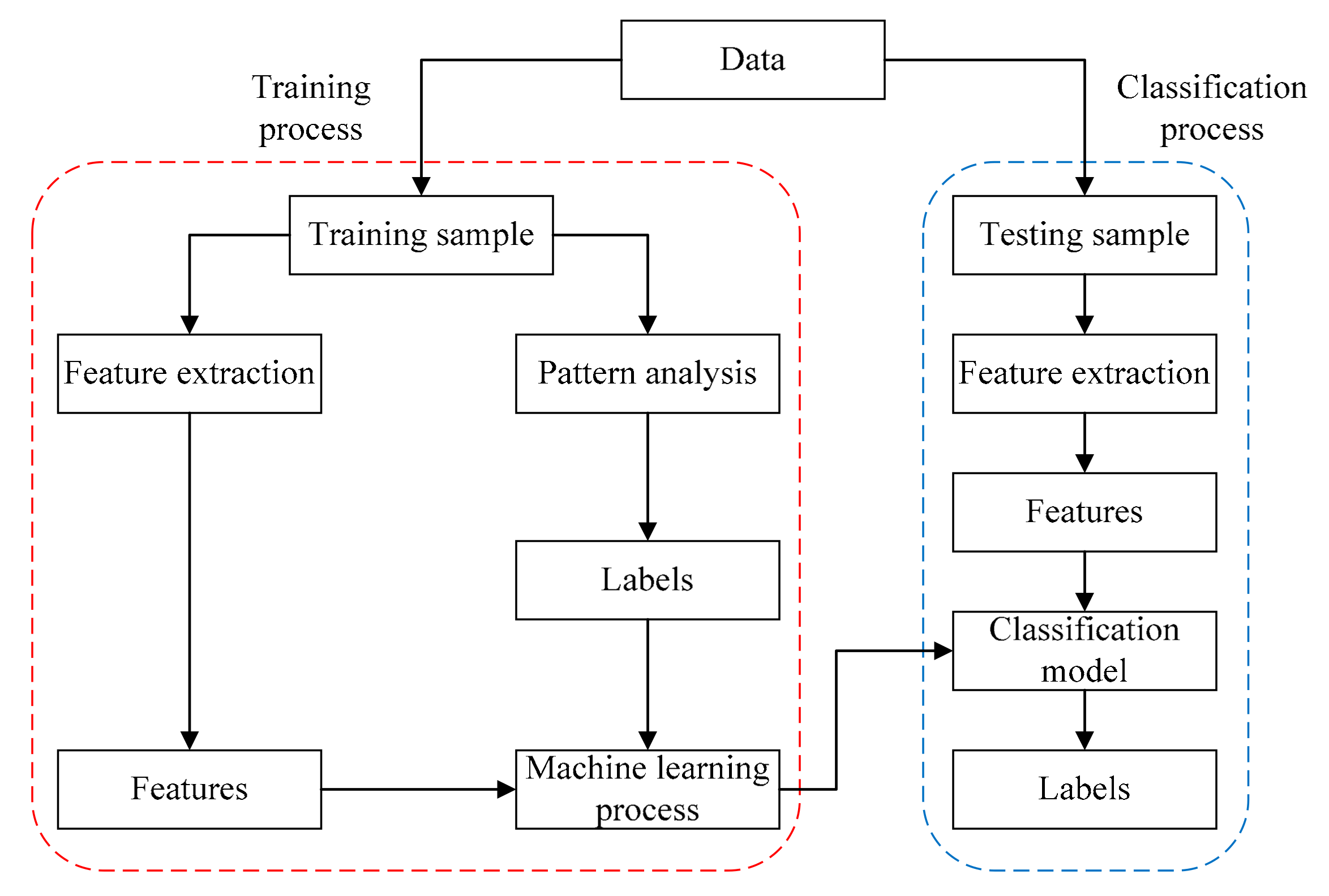
Figure 1 shows the process of solving a classification problem. The available data can be separated into two parts, of which one part is a training sample to build and train the classification model, and another is a testing sample that contains the data to be classified. For the data in the training sample, the labels are first determined by pattern analysis to distribute all data into several categories, and then the features that can describe the characteristics of different categories are also extracted.
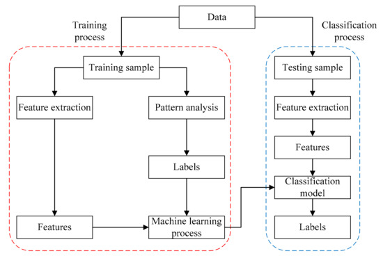
Figure 1.
Flow chart illustration of classification modeling.
We denote Fi,n as the n-th feature of sample i and Li as the label of sample i. Thus, we can represent each sample by a feature vector like Si = {Fi, Li} with Fi = {Fi,1, Fi,2, ⋯, Fi,n}. Then, the classification model is established through machine learning and training process with model inputs F and outputs L. For data in the testing sample, the features are also extracted in the same way as with the data in the training sample, and the labels can be obtained from the established classification model with the extracted features.
In the next section, a brief introduction to KNN and SVM for pattern classification is presented. The purpose of the introduction is to better understand their advantages and characteristics. As they are fairly well-known methods, a detailed derivation of these two theories will not be repeated here. KNN and SVM can also be applied in regression analysis such as forecasting [48], but the performance and model characteristics would be much different from that used in classifications.
2.2. Brief Introductions to Selected Classifiers
2.2.1. K-Nearest Neighbors
KNN is one of the most common and straightforward methods in the machine learning toolbox [49]. The simplicity of the KNN concept has made it a favorite tool for classification in different applications [50]. As an instance based learning method in pattern recognition, the KNN classifier can sort each element of a study case on account of its nearest training examples in the feature space.
For instance, to classify a sample Si, the algorithm first searches for its K nearest neighbors in the feature space depending on the feature vectors and defined distance. The algorithm then executes votes of these neighbors according to their labels. The object sample will be classified in a group with the largest number of same label neighbors. The accuracy of classification usually increases with heightened participation in votes. In general, the amount of training set data and votes mainly affect the accuracy of the KNN [51,52].
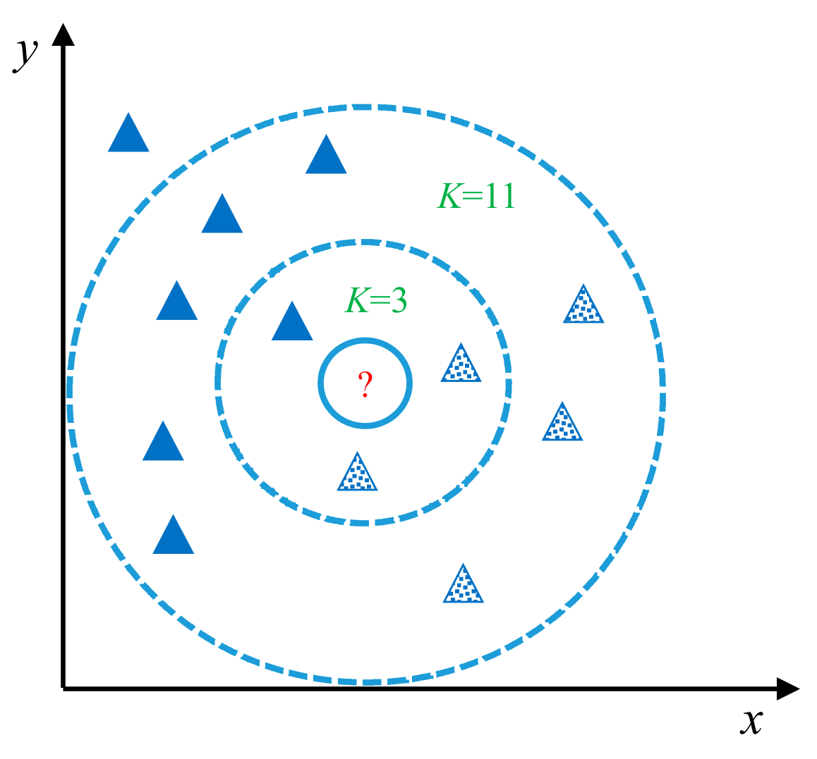
Figure 2 shows a simple demonstration of the KNN methodology. When the parameter K is equal to 3, the vote result is that the class of triangles with dots in it is in the majority. However, when the parameter K is equal to 11, the solid triangles are the majority, although the object in question (the circle in the center) is closer to the squares.
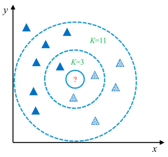
Figure 2.
Demonstration of the K-nearest neighbors (KNN) method.
This approach relies on statistics and is profoundly affected by the value of K, and thus selecting the best value for this parameter is a major problem for KNN [53]. Depending on the classification problem posed, it requires several experiments to investigate different values for the parameter K and find a value that gives proper results. Trial and error has been the dominated, but tedious, method for determining an acceptable value of K.
2.2.2. Support Vector Machines
Vapnik first proposed SVM for pattern recognition and classification [54]. By the inductive structural risk minimization principle of statistical learning theory [55,56], the SVM method is developed in such a way as to form one or a group of high or infinite dimensional hyperplanes [57,58].
The fundamental objective of SVM is to find a hyperplane to separate the points of different classes in an n-dimensional space. The distance between the hyperplane and training data point is called the functional margin, which is used to indicate the confidence of classification results. As a maximum margin classifier, the hyperplane obtained in SVM with the highest functional margin to the closest training data point provides the best data separation. The nearest training data points are called Support Vectors.
For a linearly separable problem as shown in Figure 3, the decision function is:
where is an n-dimensional vector representing the sample to be classified, is the feature vector of training sample i, = 1 or −1 if belongs to class 1 or 2, is Lagrange multiplier, and denotes the inner product operation. The belonging state of can be obtained by the sign (positive or negative) of that calculated by function (1).
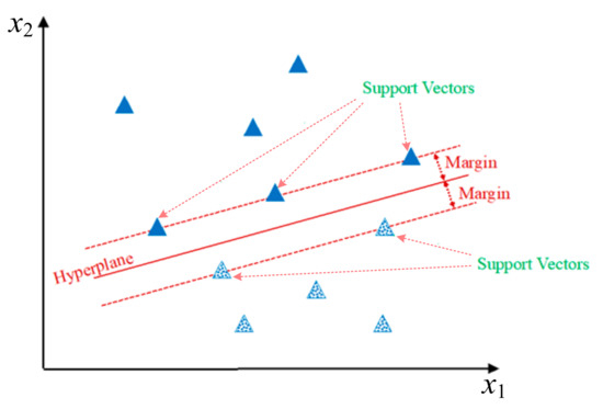
Figure 3.
An example linearly separable problem and the hyperplane that separates the data points.
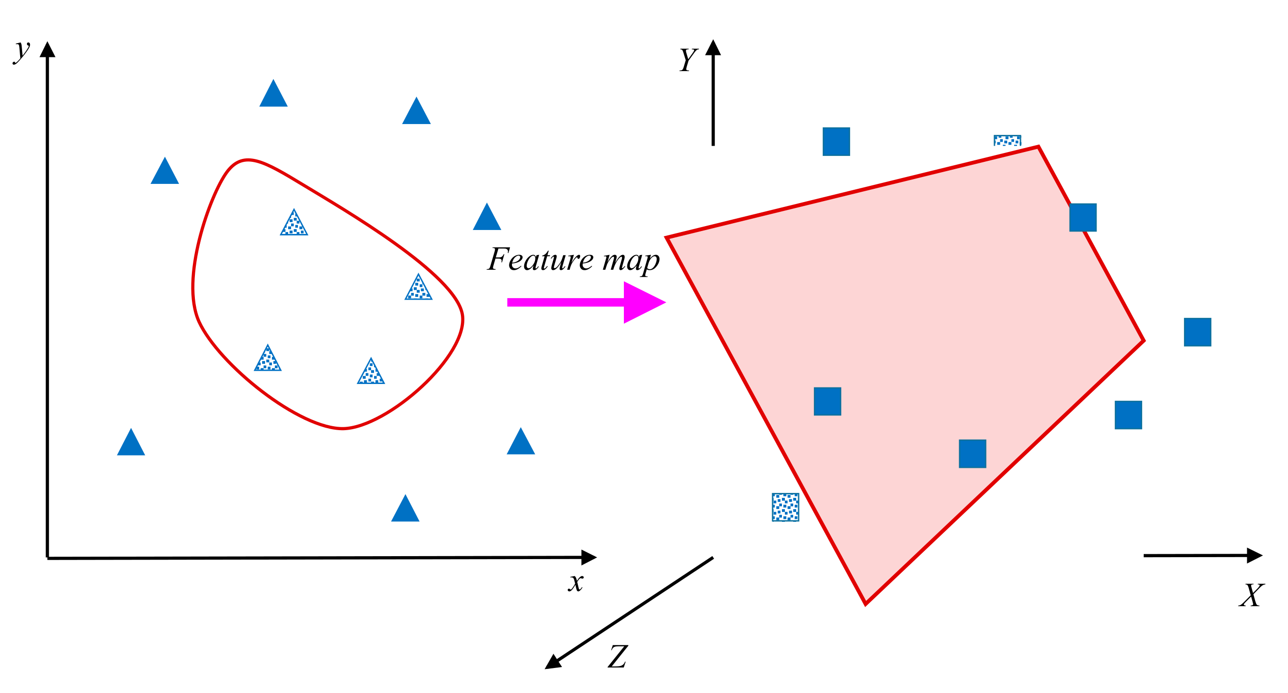
Although practical classification problems are within finite dimensions, the actual sample data discriminations are not linear and involve more complex separation approaches in that finite space. As these samples are not linearly separable, the data dimension is mapped into a higher dimensional space for possible separation, as shown in Figure 4.
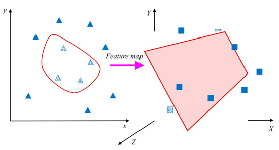
Figure 4.
The mapping of feature vectors from a low dimension (shown as triangles) to a higher dimension (shown as squares).
Then, the decision function can be rewritten as:
where indicates the mapping from the low original dimension to the higher dimension.
In the new space with higher dimension, the hyperplanes are represented as the point sets with constant dot product in the presence of a vector. The hyperplanes themselves are vectors with linear properties. As the dot product computation in larger dimensional space could be complex, the kernel function is defined to address this issue [59,60].
A kernel function satisfies:
so the inner product in a high dimension can be easily calculated by in a low dimension. Commonly used kernel functions include the linear kernel, polynomial kernel, radial basis function (RBF) kernel, sigmoid kernel, etc.
Therefore, the accuracy of SVM is related to the definition of kernel parameters and the functional margin. Small data samples can sometimes be divided into an accurate separation with proper Support Vectors, but more data points may require more complex mappings.
3. Problem Statement
Previous studies have shown that higher accuracy and better performance can be achieved by using detailed models to forecast PV power output in different weather conditions. In these works, NWP model output is an important data source for power forecasting and weather status pattern recognition. Most PV power plants in China are located in relatively remote locations, which are usually lacking in high-resolution local NWP data. Hence, to realize the classified power forecasting in different weather conditions for these PV plants, a weather classification method based on historical data of the PV plant is often required.
However, sufficient and comprehensive historical data relies on a long-term historical measured weather and power dataset, which is not generally available for a newly built PV plant. On the other hand, the weather condition at an individual PV plant is determined by regional information and seasonal factors, which means, for a given PV power plant, the data collected in some weather conditions may be plentiful while data in other weather conditions may be scarce or non-existent. This kind of imbalance in the distribution of data in different weather conditions will change as more operational data is collected.
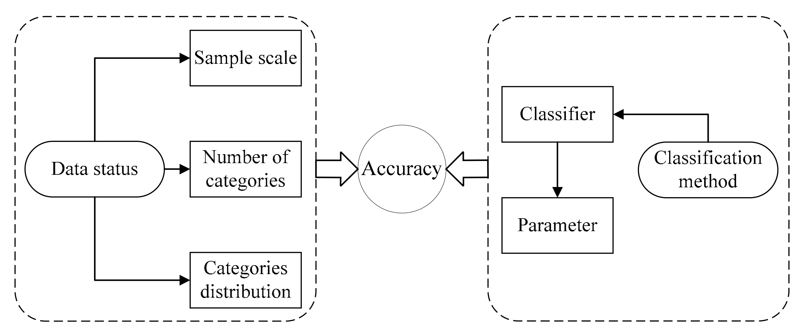
The accuracy of classification results depends both on the data status and the applied classification model and method, as shown in Figure 5. From the perspective of data status, the factors influencing accuracy can be summarized in three aspects: the sample scale of training data, the total number of categories, and the distribution of the data in different categories. From the perspective of a classification method, the factors most influencing accuracy are the classifier and the parameters of the applied classifier.

Figure 5.
Factors influencing classification accuracy.
Therefore, in the face of the different data status of an individual PV plant during the data accumulation process, multiple classification methods with optimized parameters are desperately needed. The purpose of this study is to assess the performance of SVM and KNN methods with varying data status through simulations. By analyzing and evaluating the simulation results, the mechanism of how the two factors influence classification performance can be acknowledged.
4. Case Studies
4.1. Data
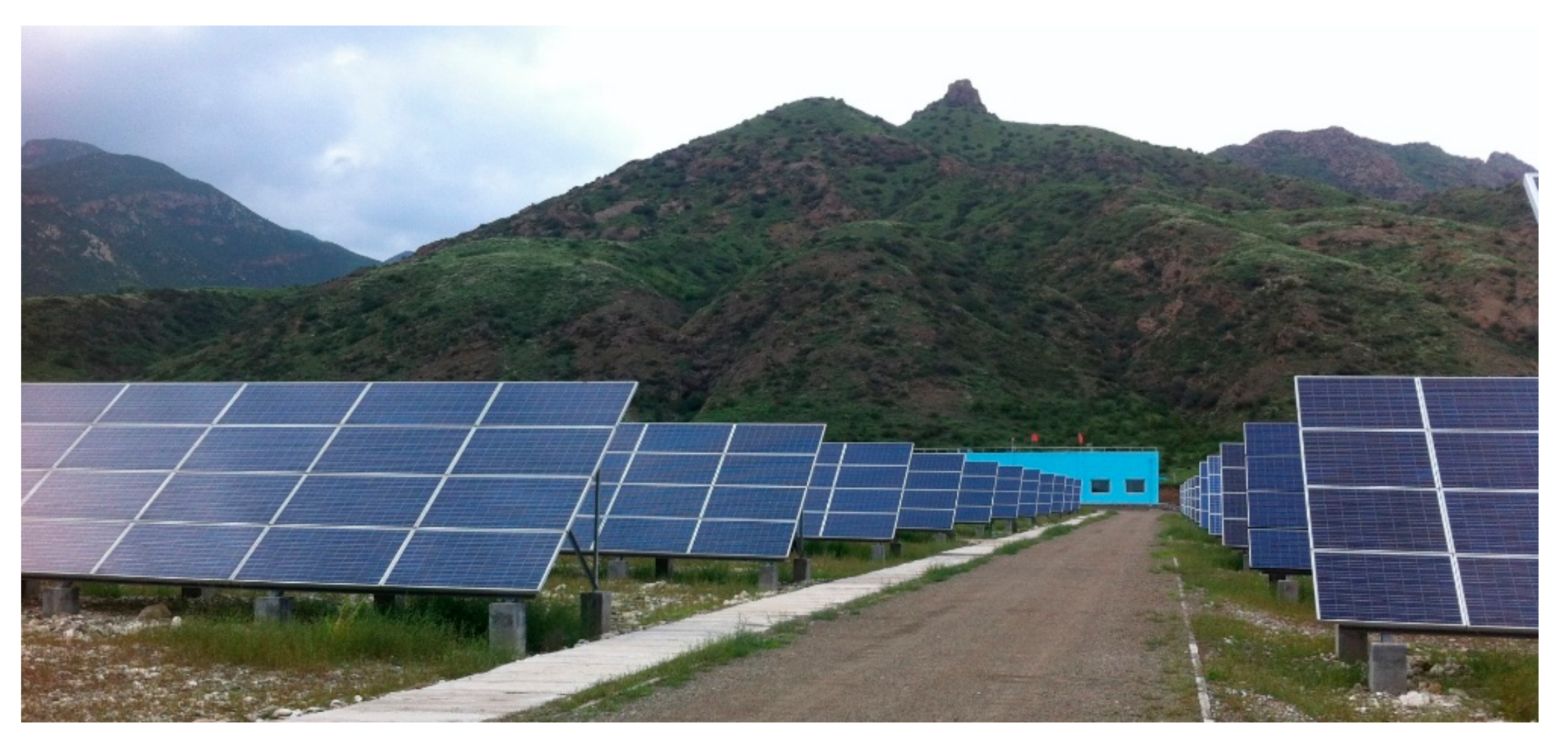
The solar irradiance data used in this paper is measured Global Horizontal Irradiance data from a grid-connected PV plant situated in Hohhot, Inner Mongolia, China (111.12° E, 40.73° N, 5 MW) from 12:00 a.m. to 11:30 p.m. with 30 min sampling interval. The time range of measuring data is from 1 January 2012 to 31 December 2012, with 310 days of available data. Figure 6 shows a photo of the grid-connected PV farm.
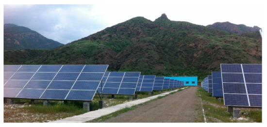
Figure 6.
The grid-connected photovoltaic (PV) farm used in the case study in this work.
The extraterrestrial solar irradiance is calculated by the following formula [61]:
where is solar constant (1368 W/m2), is the date sequence number in one year, is the date sequence number in one year, , is solar declination, is latitude and is solar hour angle.
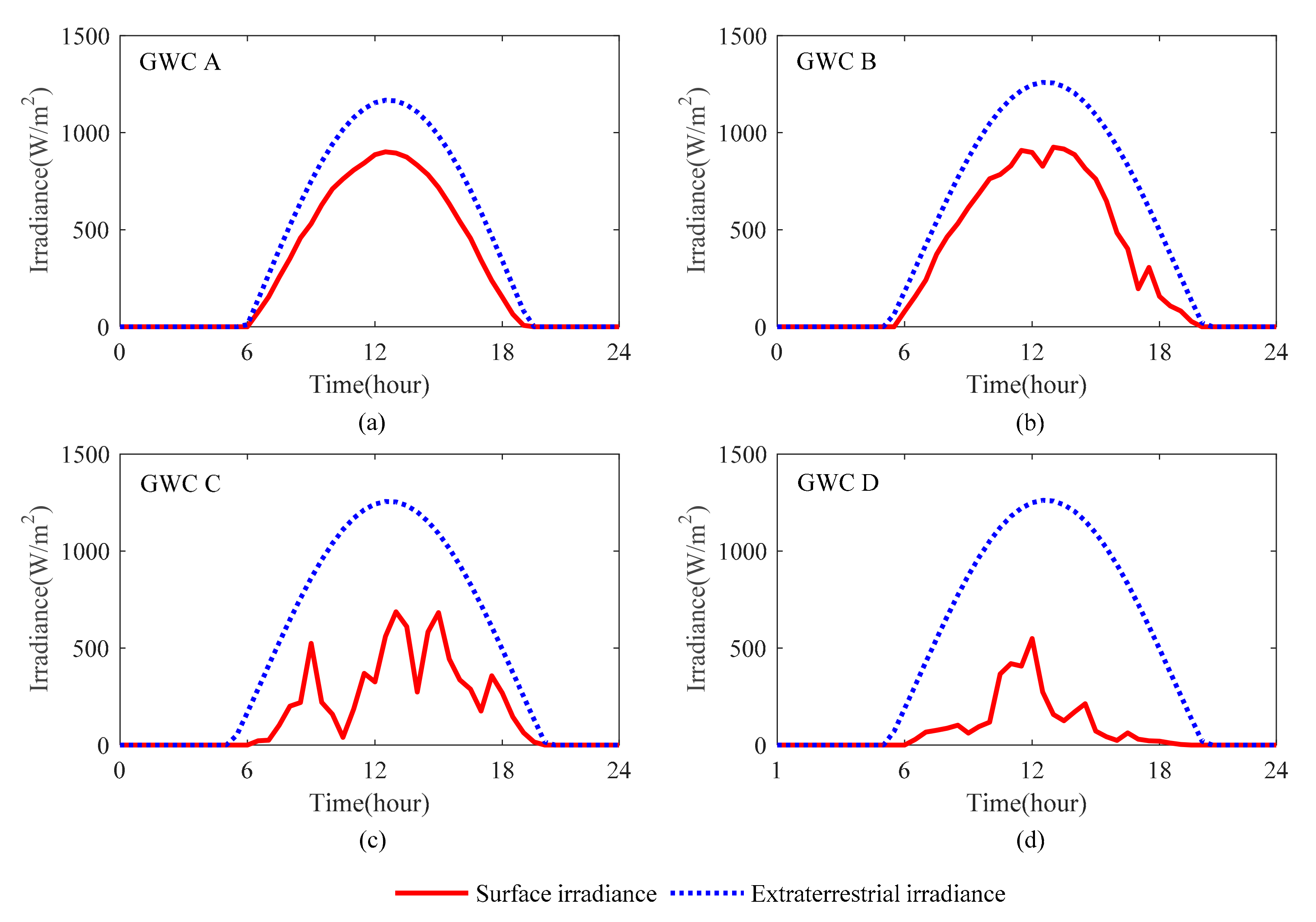
The weather status refers to the meteorological environment at the individual PV plant and can be classified into four generalized weather classes (GWC) named A, B, C and D in light of the meteorological characteristics. The typical weather patterns of the GWC A, B, C, and D can be described as: sunny, cloudy, showers, and torrential rains. By making use of the data of extraterrestrial and surface solar irradiance over a whole day, six indices reflecting the solar irradiance characteristics of different weather status are defined and calculated according to our previous study [8]:
Clearness index:
Normalized root mean square deviation:
Maximum value of third-order derivative of solar irradiance difference:
Ratio of maximum solar irradiance:
Variance of solar irradiance difference:
Inconsistency coefficient:
is the discretely sampled data of surface solar irradiance, , is the number of sample points during one day, is the corresponding extraterrestrial solar irradiance with the same fixed time interval of , . Function indicates the third-order derivative of solar irradiance difference between extraterrestrial and surface solar irradiance.
The input feature vectors for the classification model are determined as according to Formulas (5–10). The output of the model is . The resulting quantities of each GWC data bin are 24, 119, 148 and 19 as shown in Figure 7.
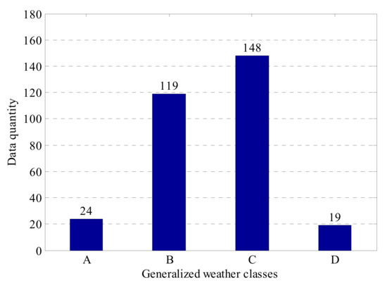
Figure 7.
The quantities of data in each generalized weather classes (GWC) weather class.
Typical surface irradiance curves (the red solid lines) with corresponding extraterrestrial irradiance curves (the blue dotted lines) of the four GWCs are illustrated in Figure 8.
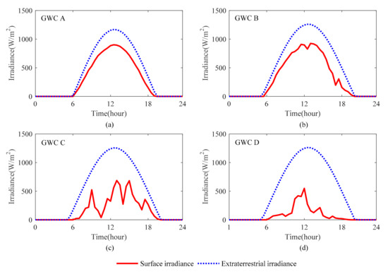
Figure 8.
Typical solar irradiance curves of four GWCs. (a) Solar irradiance curves of GWC A; (b) Solar irradiance curves of GWC B; (c) Solar irradiance curves of GWC C; (d) Solar irradiance curves of GWC D.
All the features need normalization before simulation to eliminate the influence caused by the distinction of different magnitudes. For an individual feature, it can be normalized by the following formula:
where is the original value of the feature to be normalized and is the normalized value; and are the maximum and minimum value of the feature (n = 1, 2 … or 6).
4.2. Modeling and Simulation Process
To fully utilize the data, we select each feature vector as test data in turn and choose the training data randomly among the other 309 vectors. It is important to note here that the amount of training data is one of the parameters we are examining, and thus it varies from one experiment to the next. The distribution of the four classes in the training data is required to be similar to the distribution in the entire dataset.
For the SVM method, the LibSVM software (version 3.22, Chih-Chung Chang and Chih-Jen Lin, Taipei) was used to build the classification model [62]. The C-SVC model with RBF kernel and a basic grid search method with cross-validation was used to seek out the best penalty parameter c and kernel parameter σ.
For the KNN method, the distances between all the features are calculated in Euclidean space by formula (12):
For a certain test data point, its GWC is voted on by the first K nearest neighbors in the Euclidean space of training data. In most cases, there will be only two GWCs participating in the vote due to the distribution of feature vectors. Therefore, K should be an odd number to prevent a tied vote.
The particular simulation process utilized in this work is shown in Figure 9 and can be summarized in the following steps:
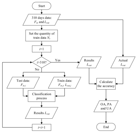
Figure 9.
The process of the simulation program.
- Step 1. Select the sample data day (i = 1, 2 …or 310).
- Step 2. Select training data among the rest of the 309 days with an approximate GWC ratio of A, B, C and D at 24:119:148:19.
- Step 3. Estimate the GWC of the selected sample data with the SVM and KNN methods.
- Step 4. Record the classification results with different sample data (), different training data quantity (), different methods (SVM or KNN) and different parameter K of KNN (K = 1, 3…, 21).
- Step 5. Calculate the performance indexes of the recorded results.
A confusion matrix, as defined in formula (13), is applied to describe the classification results:
where is the number of objects that belong to the class i but are classified into the class j, and K is the number of total categories.
Three indexes are calculated based on the confusion matrix to evaluate the performance from different perspectives:
Overall accuracy (OA)
Product’s accuracy (PA)
User’s accuracy (UA)
The overall accuracy (OA) is the indicator to describe the classification accuracy of all the outputs. The product’s accuracy (PA) and user’s accuracy (UA), respectively, evaluate the performance from the tester and user’s points of view. For a tester, the actual class of a sample is known, and the PA is used to describe the accuracy of this particular class. For users, they are more concerned about if the given classification result is correct and UA can be used to characterize the credibility of the output.
Step 6. Repeat the above steps 1–5 one hundred times, with the training data being selected randomly. The randomness of training data may lead to a one-sided model and result, so we try to reduce this randomness by multiple computing and then taking the average.
Step 7. Calculate the mean value of OA, PA, and UA with different training data quantity Nt, various methods (SVM or KNN) and different parameter K of KNN.
In the next section, we implement a series of simulations and discussions to elucidate how the factors mentioned above influence the classification accuracy. Firstly, a global comparison between the accuracy of KNN and SVM method is made. Secondly, the influences of sample scale and categories are studied to investigate the performance of the two approaches. Finally, to optimize the parameter and achieve the highest performance of the KNN classification model, the relationship between the performance and parameter setting of KNN method is also studied.
5. Results and Discussion
5.1. Global Comparison
In this section, a comprehensive comparison between SVM and KNN in different situations is conducted to achieve a basic understanding of their classification performance. The factors influencing classification accuracy for the KNN method considered in this paper are: the quantity of training data and the value of parameter K. For the SVM method, we only consider the sample scale.
Figure 10, Figure 11, Figure 12 and Figure 13 show the global performance of the SVM and KNN methods for all categories. In Figure 10, the OA of KNN varies with the value of parameter K and the quantity of training data. The accuracy of KNN is less sensitive to the quantity of training data when parameter K has a small value. However, with an increase in K, the value of OA shows significant changes with the training data quantity: a lower accuracy with small sample scales and a higher accuracy with large sample scale. In Figure 11, the OA of SVM is added in Figure 10, shown as the white plane. The performance of SVM is more stable than KNN as its accuracy plane is flat and is also higher than for the KNN method in most situations.
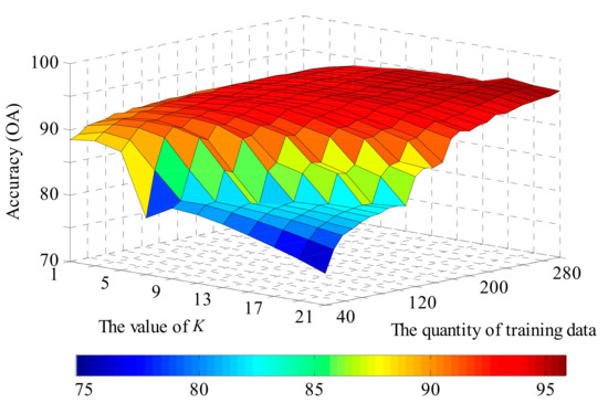
Figure 10.
The accuracy of KNN method over different values of the K parameter and training data sample scales.
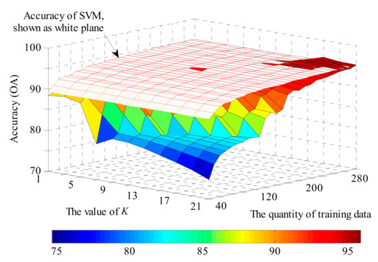
Figure 11.
The accuracy of KNN compared with the support vector machines (SVM) method.
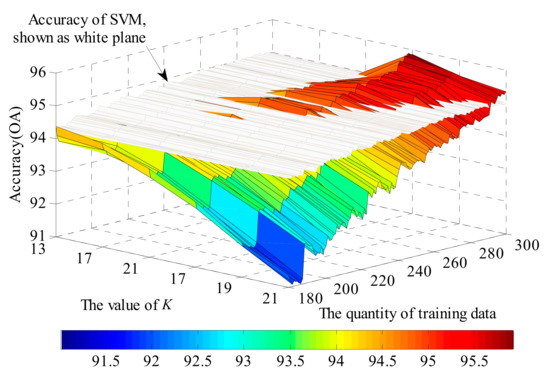
Figure 12.
Detailed view of the accuracy of KNN and SVM method for high values of K and large amounts of training data.
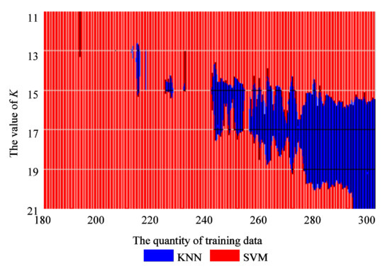
Figure 13.
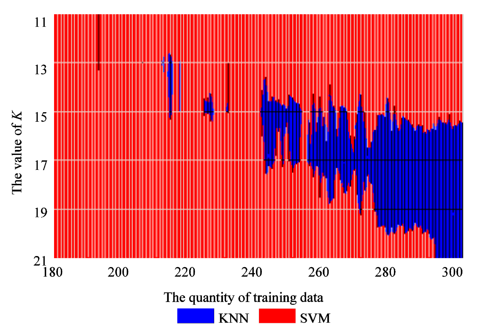
The better performing method in different parameter regions.
The KNN method shows its potential to achieve a higher classification performance with the increase in training data quantity and a suitable parameter K, as shown in the right corner of Figure 11. Figure 12 and Figure 13 show a more detailed version of the comparison with the value of K from 11 to 21 and the quantity of training data from 180 to 300. It is also apparent that the region where KNN has better performance than SVM shows an expanding trend in Figure 13, and thus is likely to have superior performance if more training data was available.
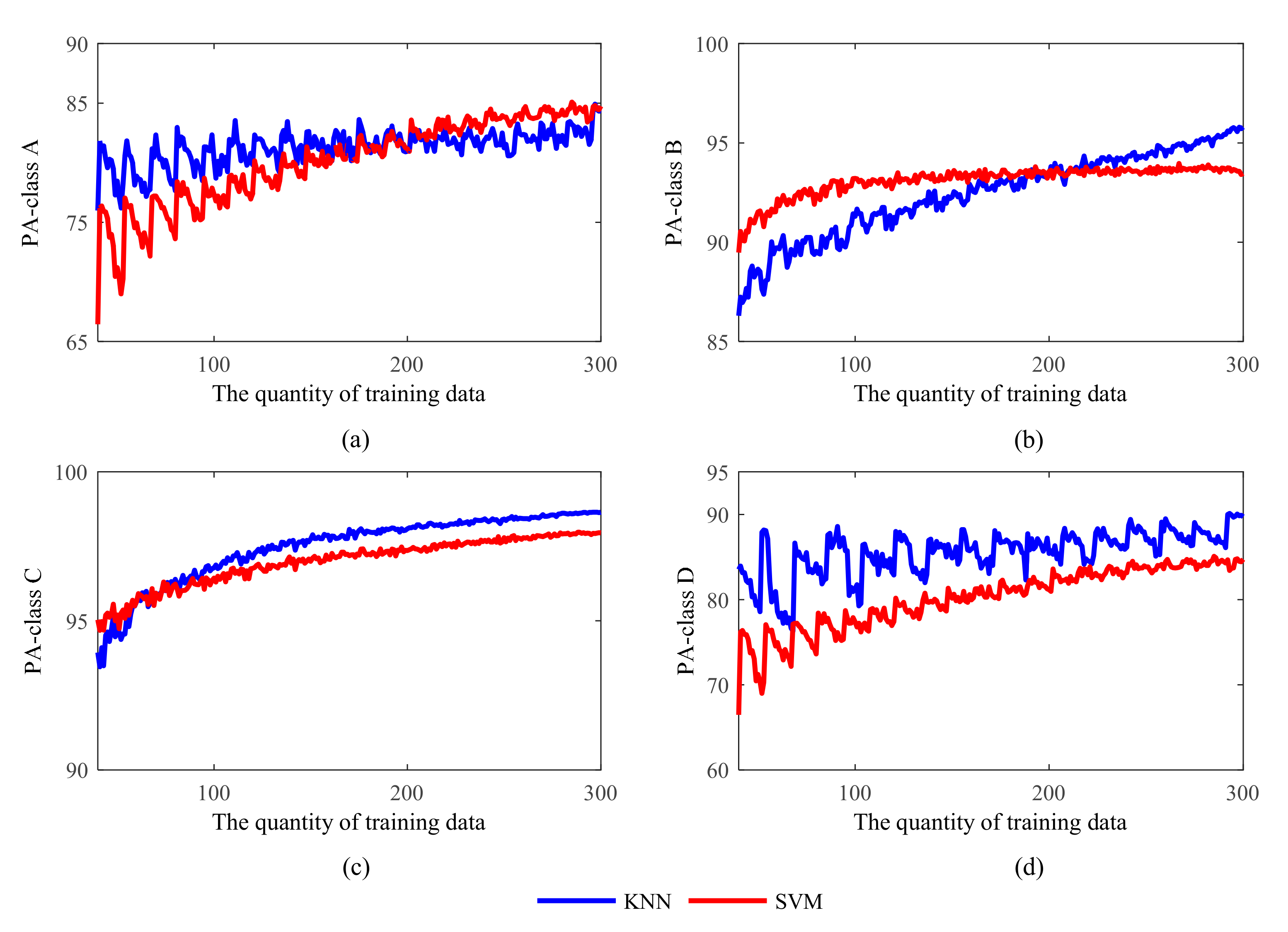
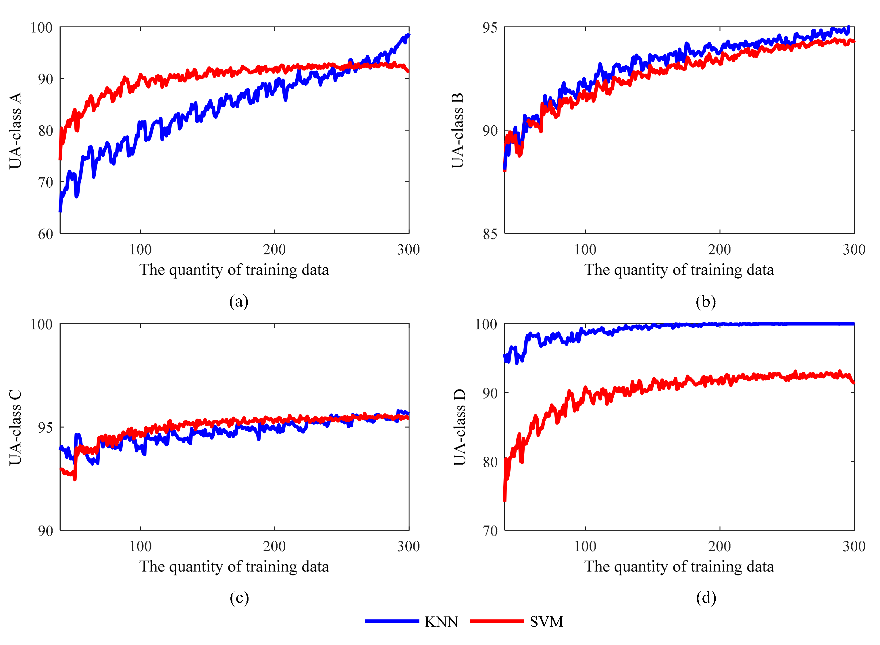
Figure 14 and Figure 15 show the comparison between the two methods, in terms of PA and UA, for the four different GWCs. The accuracy values of KNN and SVM for weather classes B and C are similar, while there are significant differences when it comes to weather classes A and D.

Figure 14.
The Product’s accuracy (PA) of KNN and SVM of four generalized weather classes. (a) PA values of GWC A; (b) PA values of GWC B; (c) PA values of GWC C; (d) PA values of GWC D.
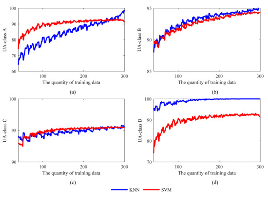
Figure 15.
The User’s accuracy (UA) of KNN and SVM of four generalized weather classes. (a) UA values of GWC A; (b) UA values of GWC B; (c) UA values of GWC C; (d) UA values of GWC D.
For class A, the highest PA values for the KNN and SVM are 84.92% and 85.08%, respectively. These two values are fairly close and so this is likely not a discriminating factor. However, the rising trends of UA are much more evident, especially for the KNN method. The UA of KNN in class A increases from 64.08% to 98.69% while the UA of SVM increases from 74.16 to 93.12% and nearly stops when the quantity of training data is more than 120. For class B and class C, the accuracy of KNN and SVM is identical. For class D, the performance of the KNN method is much better, the highest PA is 90.11% and the highest UA is 100%, while the most senior PA and UA of SVM are 84.79% and 93.12%. These differences are likely caused by the imbalance in the distribution of data in the four GWC categories. The total quantities of samples in class A and D are 24 and 19, and it is much less than the quantities of samples in class B and C, which are 119 and 148. This makes the methods more sensitive to the training sample scale, especially for class A and D.
From the above analysis, we achieve a basic result that the KNN method has a higher potential in performance than the SVM method. When the quantity of training data is large enough, the KNN method will be able to achieve a better accuracy in the case of a proper number of nearest neighbors.
5.2. The Influence of Sample Scale
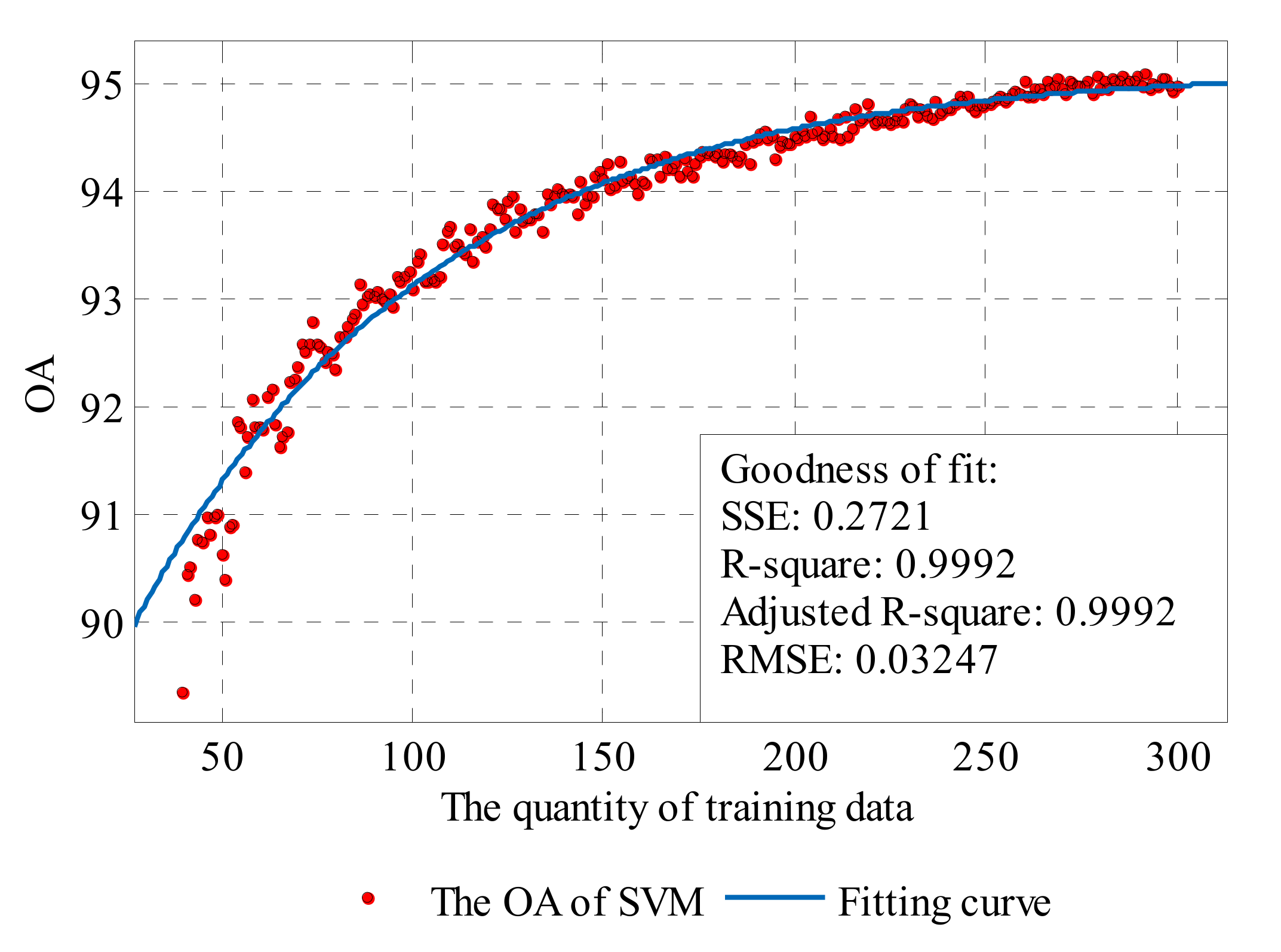
For the SVM method, the parameters are optimized before model training, so the calculated value of OA with a certain training sample scale is considered as the best accuracy directly, while, for the KNN method, the maximum value of OA obtained by different numbers of nearest neighbors—K is selected as the best accuracy. The data are illustrated in Figure 16. Then, a curve fitting for the best accuracy data is performed to quantitatively evaluate the performance and potential of KNN and SVM in data classification.
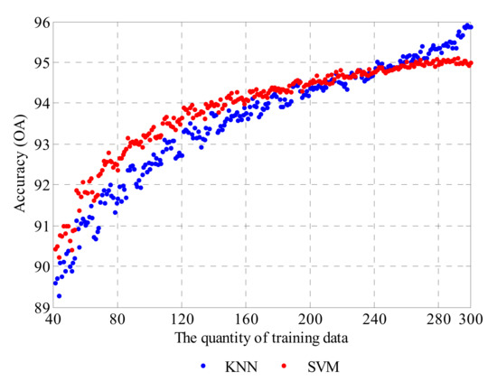
Figure 16.
The best accuracy of KNN and SVM.
Based on Figure 16, a natural exponential function is chosen as the general model:
The fitting model is a monotone increasing function with an upper bound. It contains three coefficients: is the upper bound of the function, which characterizes the maximum accuracy of the classification method, determines the increasing rate of the function, and determines the location of the zero crossing point when is certain. The curve fittings were processed by the Curve Fitting Toolbox in MATLAB (version 3.5.2, The MathWorks, Inc. Natick, MA, USA) [63].
The fitting results are shown in Table 1, and Figure 17 and Figure 18. Based on the existing data and fitting results, it can be conjectured that the highest accuracy of KNN can reach about 96.18% OA with sufficient training samples, and is superior to that of SVM, which is about 95.14% OA. The coefficient of the two methods (0.007754 for KNN and 0.01294 for SVM) illustrate that, when the training data are limited, the SVM method can achieve a relatively high accuracy rate as the increasing number of training points is more conducive to SVM. However, for the KNN method, it will need more training data to reach the same level. According to the coefficient , the accuracy rate of KNN will drop to 0 earlier than SVM when sample data are reducing.

Table 1.
The fitting results.
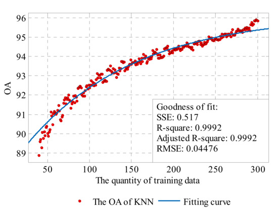
Figure 17.
The exponential curve fit to the performance results of the KNN.

Figure 18.
The exponential curve fit to the performance results of the SVM.
OAopt is the upper bound of the fitting function, R is the increasing rate of the function, and M is the location of the zero crossing point.
5.3. The Influence of Categories
Besides the training sample scale, the number of categories and the distribution of data in different categories will also affect the performance of the classifier. Four different kinds of classification cases are processed together by KNN and SVM. Case 1 is the original 4-category classification for GWC A, B, C and D. Cases 2 to 4 are three 2-category classifications, respectively, for classes A and B, classes B and C, and classes C and D. Figure 19 shows the OA differences between the two methods, i.e., the difference is equal to the OA of KNN minus the OA of SVM.
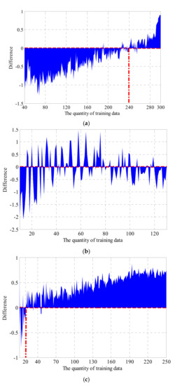
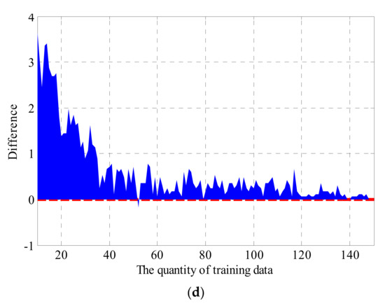
Figure 19.
The Overall accuracy (OA) difference of different classification cases: (a) case 1: OA difference of 4-category classification for GWC A, B, C and D; (b) case 2: OA difference of 2-category classification for GWC A and B; (c) case 3: OA difference of 2-category classification for GWC B and C; (d) case 4: OA difference of 2-category classification for GWC C and D.
In cases 1 and 3, the OA differences are both first less than 0 (SVM achieves a higher accuracy) and then greater than 0 (KNN achieves a higher accuracy) with the increasing of training data quantity, which is in line with the descriptions in Section 5.1 and 5.2. In Figure 19a, the zero crossing is about 240, and the quantities of four classes are 19, 92, 114 and 15, while, in Figure 19c, the zero crossing is about 20 and the quantities of classes B and C are 9 and 11. The total quantity of training data differs a lot from 240 to 20 in these two situations. The sizes of the smallest categories, 15 and 9 respectively, are relatively close. It appears that it is the quantity of data in the smallest category that matters rather than the total quantity of all training data.
However, for case 2 and case 4, it is hard to single out a similar statistical characteristic due to the significant disparity in sample scale of different categories and the lack of data of classes A and D.
5.4. The Optimal Value of the Nearest Neighbors for KNN
From our previous discussions, it can be seen that, when the parameters are fixed, the accuracy of the SVM model can be maintained to a certain extent no matter if the quantity of training data is decreased or increased. This makes it feasible to use the cross-validation for parameter optimization and apply the same optimized parameters to all simulations. However, for the KNN method, the OA value varies significantly with the training data under a particular parameter K (number of nearest neighbors) while the cross-validation needs to separate the whole training data into small samples. Thus, it is impossible to optimize the parameter of KNN by using this kind of method.
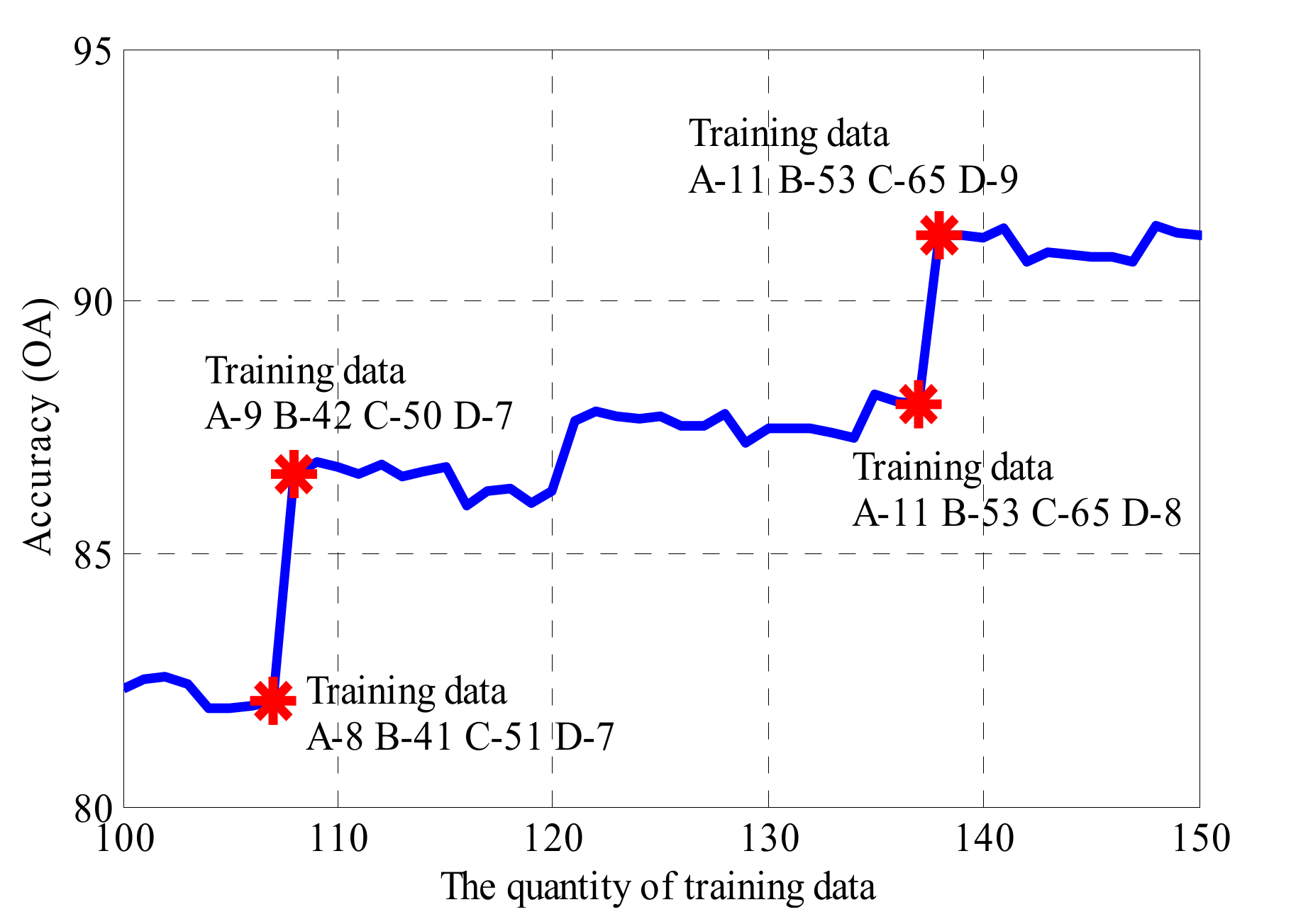
Section 5.3 indicates a possibility that the quantity of data in the smallest category determines the accuracy of the KNN method. To further verify this possibility, Figure 20 shows the variation of the 17-KNN method with training data quantity from 100 to 150. It can be seen that there are two jumps in accuracy with the increase in training data. The first jump is from 82.07% OA to 86.55% OA at the place of 107 training data (A-8, B-41, C-51, D-7) to 108 training data (A-9, B-42, C-50, D-7). The second jump is from 87.97% OA to 91.28% OA at the place of 137 training data (A-11, B-53, C-65, D-8) to 138 training data (A-10, B-53, C-65, D-9). The similarity of these two jumping points is that the amount of a particular class of data increases from 8, which is less than half of 17 (the value of K) to 9, which is more than the half of K. This suggests that the possibility to be the absolute majority in voting of a certain GWC is a prerequisite for increased accuracy. Thus, to achieve the highest accuracy, the minimum condition is that the smallest GWC can be the absolute majority in voting, i.e., the sample scale of the smallest GWC needs to be more than half of the nearest neighbors.

Figure 20.
The OA of the KNN method when K = 17.
Figure 21 shows the K-OA curves with different sample scales. All four of the curves show a trend that first increases and then decreases with increasing values of K. It is worth noting that the position of the vertex corresponds with the quantity of the smallest category: for each curve, it will reach its maximum when the value of K is around the quantity of the smallest category.
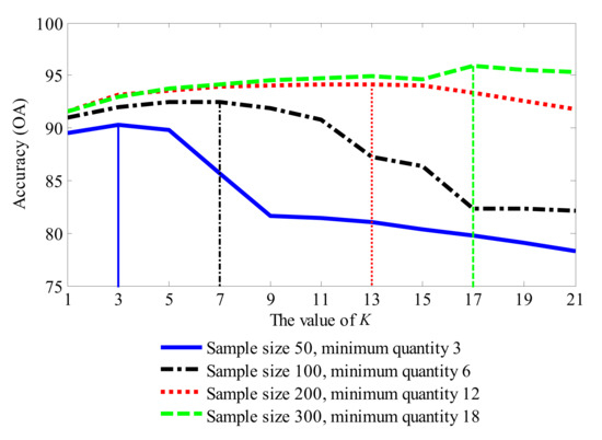
Figure 21.
The K-OA curves with different sample scale.
To further validate this correspondence between K and the quantity of training data, we compare the optimal value of the nearest neighbors Kopt that can achieve the highest accuracy (OA) and the minimum quantity of four GWCs with different training sample scales in Figure 22.
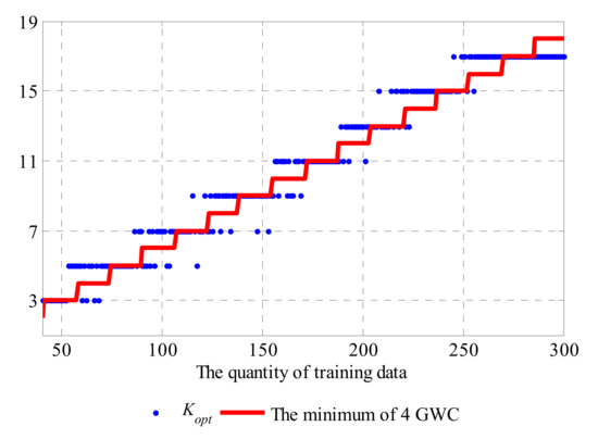
Figure 22.
Kopt and the minimum quantity of the four GWC training samples with different overall training sample scales.
In general, Kopt increases with the training data quantity although there may be some fluctuations. The minimum quantity of four GWCs also shows a high correlation with the best value of K. The values of the minimum quantity of four GWCs can be fitted by function (18) to bring them into correspondence with the domain of K:
The correlation coefficient of Kopt and the fitted minimum quantity of 4 GWC is 0.9777, and the root mean square error (RMSE) between them is only 1.0057. This means that, for a classification problem with an imbalance in distributed samples such as that in our study, the best value of parameter K mainly depends on the quantity of class with the smallest sample scale. Thus, for the PV plant considered in this paper, the suggested value of K with a particular sample scale can be:
where NA, NB, NC and ND refer to the quantities of data in each GWC.
5.5. Summary
According to the previous simulations and discussions, the following points are worth noting:
- If all the data or the majority of data are balanced across different categories, the performance of classifier will be significantly correlated with the training data scale.
- The SVM method can achieve a relatively high performance with small sample scales, while the KNN is not applicable in this situation. However, the KNN method has a better potential and a higher upper limit of accuracy in classification than the SVM. With increases in training sample scale, the performance of the KNN method will have a significant improvement, and the performance of SVM will stagnate after a certain degree of growth.
- For the KNN method, the accuracy and the optimal parameter K are all mainly dependent on the size of the smallest category.
6. Conclusions
In order to figure out which classifiers are more suitable for the weather classification models of DAST solar PV power forecasting under various circumstances, we investigate, compare and evaluate the influences of different machine learning classification methods and data statuses on classification accuracy in this paper. The simulation results based on two common used classification methods (i.e., KNN and SVM) illustrate that SVM achieved higher classification accuracy and more robustness performance than KNN under small sample data scales, while KNN showed the potential and finally exceeds in accuracy with the increase of training sample scales. This trend became more evident in the case of balanced data distribution than unbalanced data. For the KNN method, the number of nearest neighbors matters as well besides the sample scale, of which the optimal number is proportional to the quantity of the smallest category.
The conclusions verified the merits of SVM that usually an accurate separation could be approached only using a comparative small amount of data by taking advantage of hyperplanes to separate data points in a high dimensional space through the characteristic mapping realized by appropriate kernel functions. At the same time, it also indicated that the influence of the amount and scale of the training dataset is much more significant to KNN than to SVM, which are also in accordance with the basic principle of KNN that the label of certain data point is determined by the majority of its neighboring points. Therefore, SVM is prioritized for weather status pattern classification of DAST solar PV power forecasting because of its advantage in dealing with small sample scales for those newly built PV plants lacking in historical data. As more data is available, the KNN classifier could become more accurate and needs to be taken into consideration. The feasibility and comparison research on the application of other machine learning classification methods for DAST solar PV power forecasting weather classification models, such as K-means, Adaptive Boosting and Random Forest, will be the future works subsequently.
Acknowledgments
This work was supported partially by the National Natural Science Foundation of China (Grant No. 51577067), the National Key Research and Development Program of China (Grant No. 2017YFF0208106), the Beijing Natural Science Foundation of China (Grant No. 3162033), the Beijing Science and Technology Program of China (Grant No. Z161100002616039), the Hebei Natural Science Foundation of China (Grant No. E2015502060), the State Key Laboratory of Alternate Electrical Power System with Renewable Energy Sources (Grant Nos. LAPS16007, LAPS16015), the Science and Technology Project of State Grid Corporation of China (SGCC), the Open Fund of State Key Laboratory of Operation and Control of Renewable Energy and Storage Systems (China Electric Power Research Institute) (No. 5242001600FB) and the China Scholarship Council.
Author Contributions
Fei Wang and Zengqiang Mi conceived and designed the experiments; Zhao Zhen performed the experiments and analyzed the data; Bo Wang contributed reagents/materials/analysis tools; Zhao Zhen and Fei Wang wrote the paper.
Conflicts of Interest
The authors declare that the grant, scholarship, and/or funding mentioned in the Acknowledgments section do not lead to any conflict of interest. Additionally, the authors declare that there is no conflict of interest regarding the publication of this manuscript.
References
- Pandey, A.K.; Tyagi, V.V.; Selvaraj, J.A.; Rahim, N.A.; Tyagi, S.K. Recent advances in solar photovoltaic systems for emerging trends and advanced applications. Renew. Sustain. Energy Rev. 2016, 53, 859–884. [Google Scholar] [CrossRef]
- Turkay, B.E.; Telli, A.Y. Economic analysis of standalone and grid connected hybrid energy systems. Renew. Energy 2011, 36, 1931–1943. [Google Scholar] [CrossRef]
- International Energy Agency (IEA). IEA Energy Technology Perspectives 2014. International Energy Agency (IEA): Paris, France, 2014. [Google Scholar]
- International Energy Agency (IEA). Excerpt from Renewables Information, 2015 ed. International Energy Agency (IEA): Paris, France, 2015. [Google Scholar]
- International Energy Agency (IEA). Technology Roadmap, Solar Photovoltaic Energy, 2014 ed. International Energy Agency (IEA): Paris, France, 2014. [Google Scholar]
- Chen, Q.; Wang, F.; Hodge, B.-M.; Zhang, J.; Li, Z.; Shafie-Khah, M.; Catalao, J.P.S. Dynamic Price Vector Formation Model-Based Automatic Demand Response Strategy for PV-Assisted EV Charging Stations. IEEE Trans. Smart Grid 2017, 8, 2903–2915. [Google Scholar] [CrossRef]
- Peng, J.; Lu, L. Investigation on the development potential of rooftop PV system in Hong Kong and its environmental benefits. Renew. Sustain. Energy Rev. 2013, 27, 149–162. [Google Scholar] [CrossRef]
- Wang, F.; Zhen, Z.; Mi, Z.; Sun, H.; Su, S.; Yang, G. Solar irradiance feature extraction and support vector machines based weather status pattern recognition model for short-term photovoltaic power forecasting. Energy Build. 2015, 86, 427–438. [Google Scholar] [CrossRef]
- Kheshti, M.; Yeripour, M.N.; Majidpour, M.D. Fuzzy dispatching of solar energy in distribution system. Appl. Sol. Energy 2011, 47, 105–111. [Google Scholar] [CrossRef]
- Diagne, M.; David, M.; Lauret, P.; Boland, J.; Schmutz, N. Review of solar irradiance forecasting methods and a proposition for small-scale insular grids. Renew. Sustain. Energy Rev. 2013, 27, 65–76. [Google Scholar] [CrossRef]
- Wang, F.; Xu, H.; Xu, T.; Li, K.; Shafie-khah, M.; Catalão, J.P.S. The values of market-based demand response on improving power system reliability under extreme circumstances. Appl. Energy 2017, 193, 220–231. [Google Scholar] [CrossRef]
- Orwig, K.D.; Ahlstrom, M.L.; Banunarayanan, V.; Sharp, J.; Wilczak, J.M.; Freedman, J.; Haupt, S.E.; Cline, J.; Bartholomy, O.; Hamann, H.F.; et al. Recent Trends in Variable Generation Forecasting and Its Value to the Power System. Sol. Energy 2014, 6, 192–203. [Google Scholar] [CrossRef]
- Brancucci Martinez-Anido, C.; Botor, B.; Florita, A.R.; Draxl, C.; Lu, S.; Hamann, H.F.; Hodge, B.M. The value of day-ahead solar power forecasting improvement. Sol. Energy 2016, 129, 192–203. [Google Scholar] [CrossRef]
- Zhang, J.; Florita, A.; Hodge, B.-M.; Lu, S.; Hamann, H.F.; Banunarayanan, V.; Brockway, A.M. A suite of metrics for assessing the performance of solar power forecasting. Sol. Energy 2015, 111, 157–175. [Google Scholar] [CrossRef]
- Tuohy, A.; Zack, J.; Haupt, S.E.; Sharp, J.; Ahlstrom, M.; Dise, S.; Grimit, E.; Mohrlen, C.; Lange, M.; Casado, M.G.; et al. Solar Forecasting: Methods, Challenges, and Performance. IEEE Power Energy Mag. 2015, 13, 50–59. [Google Scholar] [CrossRef]
- Kleissl, J.; Coimbra, C.F.M.; Pedro, H.T.C. Solar Energy Forecasting and Resource Assessment; Academic Press: Cambridge, MA, USA, 2013. [Google Scholar]
- Pelland, S.; Remund, J.; Kleissl, J.; Oozeki, T.; De Brabandere, K. Photovoltaic and Solar Forecasting: State of the Art. IEA PVPS Task 2013, 14, 1–36. [Google Scholar]
- Bernecker, D.; Riess, C.; Angelopoulou, E.; Hornegger, J. Continuous short-term irradiance forecasts using sky images. Sol. Energy 2014, 110, 303–315. [Google Scholar] [CrossRef]
- Alonso-Montesinos, J.; Batlles, F.J.; Portillo, C. Solar irradiance forecasting at one-minute intervals for different sky conditions using sky camera images. Energy Convers. Manag. 2015, 105, 1166–1177. [Google Scholar] [CrossRef]
- Wang, F.; Zhen, Z.; Liu, C.; Mi, Z.; Hodge, B.-M.; Shafie-khah, M.; Catalão, J.P.S. Image phase shift invariance based cloud motion displacement vector calculation method for ultra-short-term solar PV power forecasting. Energy Convers. Manag. 2018, 157, 123–135. [Google Scholar] [CrossRef]
- Marquez, R.; Pedro, H.T.C.; Coimbra, C.F.M. Hybrid solar forecasting method uses satellite imaging and ground telemetry as inputs to ANNs. Sol. Energy 2013, 92, 176–188. [Google Scholar] [CrossRef]
- Polo, J.; Wilbert, S.; Ruiz-Arias, J.A.; Meyer, R.; Gueymard, C.; Súri, M.; Martín, L.; Mieslinger, T.; Blanc, P.; Grant, I.; et al. Preliminary survey on site-adaptation techniques for satellite-derived and reanalysis solar radiation datasets. Sol. Energy 2016, 132, 25–37. [Google Scholar] [CrossRef]
- Dong, Z.; Yang, D.; Reindl, T.; Walsh, W.M. Satellite image analysis and a hybrid ESSS/ANN model to forecast solar irradiance in the tropics. Energy Convers. Manag. 2014, 79, 66–73. [Google Scholar] [CrossRef]
- Chow, C.W.; Urquhart, B.; Lave, M.; Dominguez, A.; Kleissl, J.; Shields, J.; Washom, B. Intra-hour forecasting with a total sky imager at the UC San Diego solar energy testbed. Sol. Energy 2011, 85, 2881–2893. [Google Scholar] [CrossRef]
- Sun, Y.; Wang, F.; Wang, B.; Chen, Q.; Engerer, N.A.; Mi, Z. Correlation Feature Selection and Mutual Information Theory Based Quantitative Research on Meteorological Impact Factors of Module Temperature for Solar Photovoltaic Systems. Energies 2016, 10, 7. [Google Scholar] [CrossRef]
- Akarslan, E.; Hocaoglu, F.O. A novel adaptive approach for hourly solar radiation forecasting. Renew. Energy 2016, 87, 628–633. [Google Scholar] [CrossRef]
- Soubdhan, T.; Ndong, J.; Ould-Baba, H.; Do, M.T. A robust forecasting framework based on the Kalman filtering approach with a twofold parameter tuning procedure: Application to solar and photovoltaic prediction. Sol. Energy 2016, 131, 246–259. [Google Scholar] [CrossRef]
- Fatemi, S.A.; Kuh, A.; Fripp, M. Online and batch methods for solar radiation forecast under asymmetric cost functions. Renew. Energy 2016, 91, 397–408. [Google Scholar] [CrossRef]
- Wang, F.; Mi, Z.; Su, S.; Zhao, H. Short-term solar irradiance forecasting model based on artificial neural network using statistical feature parameters. Energies 2012, 5, 1355–1370. [Google Scholar] [CrossRef]
- Aybar-Ruiz, A.; Jiménez-Fernández, S.; Cornejo-Bueno, L.; Casanova-Mateo, C.; Sanz-Justo, J.; Salvador-González, P.; Salcedo-Sanz, S. A novel Grouping Genetic Algorithm–Extreme Learning Machine approach for global solar radiation prediction from numerical weather models inputs. Sol. Energy 2016, 132, 129–142. [Google Scholar] [CrossRef]
- Perez, R.; Lorenz, E.; Pelland, S.; Beauharnois, M.; Van Knowe, G.; Hemker, K.; Heinemann, D.; Remund, J.; Müller, S.C.; Traunmüller, W.; et al. Comparison of numerical weather prediction solar irradiance forecasts in the US, Canada and Europe. Sol. Energy 2013, 94, 305–326. [Google Scholar] [CrossRef]
- Obara, S.Y.; El-Sayed, A.G. Compound microgrid installation operation planning of a PEFC and photovoltaics with prediction of electricity production using GA and numerical weather information. Int. J. Hydrog. Energy 2009, 34, 8213–8222. [Google Scholar] [CrossRef]
- Verzijlbergh, R.A.; Heijnen, P.W.; de Roode, S.R.; Los, A.; Jonker, H.J.J. Improved model output statistics of numerical weather prediction based irradiance forecasts for solar power applications. Sol. Energy 2015, 118, 634–645. [Google Scholar] [CrossRef]
- Ma, W.W.; Rasul, M.G.; Liu, G.; Li, M.; Tan, X.H. Climate change impacts on techno-economic performance of roof PV solar system in Australia. Renew. Energy 2016, 88, 430–438. [Google Scholar] [CrossRef]
- Huber, I.; Bugliaro, L.; Ponater, M.; Garny, H.; Emde, C.; Mayer, B. Do climate models project changes in solar resources? Sol. Energy 2016, 129, 65–84. [Google Scholar] [CrossRef]
- Belaid, S.; Mellit, A. Prediction of daily and mean monthly global solar radiation using support vector machine in an arid climate. Energy Convers. Manag. 2016, 118, 105–118. [Google Scholar] [CrossRef]
- Zhang, Y.; Beaudin, M.; Taheri, R.; Zareipour, H.; Wood, D. Day-Ahead Power Output Forecasting for Small-Scale Solar Photovoltaic Electricity Generators. IEEE Trans. Smart Grid 2015, 6, 2253–2262. [Google Scholar] [CrossRef]
- Lima, F.J.L.; Martins, F.R.; Pereira, E.B.; Lorenz, E.; Heinemann, D. Forecast for surface solar irradiance at the Brazilian Northeastern region using NWP model and artificial neural networks. Renew. Energy 2016, 87, 807–818. [Google Scholar] [CrossRef]
- Shah, A.S.B.M.; Yokoyama, H.; Kakimoto, N. High-Precision Forecasting Model of Solar Irradiance Based on Grid Point Value Data Analysis for an Efficient Photovoltaic System. IEEE Trans. Sustain. Energy 2015, 6, 474–481. [Google Scholar] [CrossRef]
- Engerer, N.A. Minute resolution estimates of the diffuse fraction of global irradiance for southeastern Australia. Sol. Energy 2015, 116, 215–237. [Google Scholar] [CrossRef]
- Yang, H.T.; Huang, C.M.; Huang, Y.C.; Pai, Y.S. A Weather-Based Hybrid Method for 1-Day Ahead Hourly Forecasting of PV Power Output. IEEE Trans. Sustain. Energy 2014, 5, 917–926. [Google Scholar] [CrossRef]
- Shi, J.; Lee, W.J.; Liu, Y.; Yang, Y.; Wang, P. Forecasting power output of photovoltaic systems based on weather classification and support vector machines. IEEE Trans. Ind. Appl. 2012, 48, 1064–1069. [Google Scholar] [CrossRef]
- Chen, C.S.; Duan, S.X.; Cai, T.; Liu, B.Y. Online 24-h solar power forecasting based on weather type classification using artificial neural network. Sol. Energy 2011, 85, 2856–2870. [Google Scholar] [CrossRef]
- Larson, D.P.; Nonnenmacher, L.; Coimbra, C.F.M. Day-ahead forecasting of solar power output from photovoltaic plants in the American Southwest. Renew. Energy 2016, 91, 11–20. [Google Scholar] [CrossRef]
- Nonnenmacher, L.; Kaur, A.; Coimbra, C.F.M. Day-ahead resource forecasting for concentrated solar power integration. Renew. Energy 2016, 86, 866–876. [Google Scholar] [CrossRef]
- Hmeidi, I.; Hawashin, B.; El-Qawasmeh, E. Performance of KNN and SVM classifiers on full word Arabic articles. Adv. Eng. Informat. 2008, 22, 106–111. [Google Scholar] [CrossRef]
- Alpaydın, E. Introduction to Machine Learning; MIT Press: Cambridge, MA, USA, 2014; Volume 1107. [Google Scholar]
- Wolff, B.; Lorenz, E.; Kramer, O. Statistical Learning for Short-Term Photovoltaic Power Predictions. In Computational Sustainability; Springer International Publishing: Berlin, Germany, 2016; pp. 31–45. [Google Scholar]
- Cover, T.; Hart, P. Nearest neighbor pattern classification. IEEE Trans. Inf. Theory 1967, 13, 21–27. [Google Scholar] [CrossRef]
- Denoeux, T. A k-nearest neighbor classification rule based on Dempster-Shafer theory. IEEE Trans. Syst. Man Cybern. 1995, 25, 804–813. [Google Scholar] [CrossRef]
- Lanjewar, R.B.; Mathurkar, S.; Patel, N. Implementation and Comparison of Speech Emotion Recognition System Using Gaussian Mixture Model (GMM) and K-Nearest Neighbor (K-NN) Techniques. Procedia Comput. Sci. 2015, 49, 50–57. [Google Scholar] [CrossRef]
- Aburomman, A.A.; Ibne Reaz, M. Bin A novel SVM-kNN-PSO ensemble method for intrusion detection system. Appl. Soft Comput. J. 2016, 38, 360–372. [Google Scholar] [CrossRef]
- Zhang, H.; Berg, A.C.; Maire, M.; Malik, J. SVM-KNN: Discriminative Nearest Neighbor Classification for Visual Category Recognition. In Proceedings of the IEEE Computer Society Conference on Computer Vision and Pattern Recognition, New York, NY, USA, 17–22 June 2006; Volume 2, pp. 2126–2136. [Google Scholar]
- Cortes, C.; Vapnik, V. Support-Vector Networks. Mach. Learn. 1995, 20, 273–297. [Google Scholar] [CrossRef]
- Vapnik, V.N. Statistical Learning Theory; Wiley: New York, NY, USA, 1998. [Google Scholar]
- Vapnik, V. The Nature of Statistical Learning Theory; Springer Science & Business Media: Berlin, Germany, 1995. [Google Scholar]
- Melgani, F.; Bazi, Y. Classification of electrocardiogram signals with support vector machines and particle swarm optimization. IEEE Trans. Inf. Technol. Biomed. 2008, 12, 667–677. [Google Scholar] [CrossRef] [PubMed]
- Subasi, A. Classification of EMG signals using PSO optimized SVM for diagnosis of neuromuscular disorders. Comput. Biol. Med. 2013, 43, 576–586. [Google Scholar] [CrossRef] [PubMed]
- Cervantes, J.; García Lamont, F.; López-Chau, A.; Rodríguez Mazahua, L.; Sergio Ruíz, J. Data selection based on decision tree for SVM classification on large data sets. Appl. Soft Comput. 2015, 37, 787–798. [Google Scholar] [CrossRef]
- Shen, X.-J.; Mu, L.; Li, Z.; Wu, H.-X.; Gou, J.-P.; Chen, X. Large-scale support vector machine classification with redundant data reduction. Neurocomputing 2016, 172, 189–197. [Google Scholar] [CrossRef]
- Duffie, J.A.; Beckman, W.A. Solar Engineering of Thermal Processes, 4th ed.; John Wiley and Sons: New York, NY, USA, 2013. [Google Scholar]
- Chang, C.-C.; Lin, C.-J. LIBSVM: A library for support vector machines. ACM Trans. Intell. Syst. Technol. 2011, 2, 27:1–27:27. [Google Scholar] [CrossRef]
- Curve Fitting Toolbox-MATLAB. Available online: http://www.mathworks.com/products/curvefitting/?s_tid=srchtitle (accessed on 10 November 2017).
© 2017 by the authors. Licensee MDPI, Basel, Switzerland. This article is an open access article distributed under the terms and conditions of the Creative Commons Attribution (CC BY) license (http://creativecommons.org/licenses/by/4.0/).

