Abstract
Visual tracking is a challenging task in computer vision due to various appearance changes of the target object. In recent years, correlation filter plays an important role in visual tracking and many state-of-the-art correlation filter based trackers are proposed in the literature. However, these trackers still have certain limitations. Most of existing trackers cannot well deal with scale variation, and they may easily drift to the background in the case of occlusion. To overcome the above problems, we propose a Correlation Filters based Scale Adaptive (CFSA) visual tracker. In the tracker, a modified EdgeBoxes generator, is proposed to generate high-quality candidate object proposals for tracking. The pool of generated candidate object proposals is adopted to estimate the position of the target object using a kernelized correlation filter based tracker with HOG and color naming features. In order to deal with changes in target scale, a scale estimation method is proposed by combining the water flow driven MBD (minimum barrier distance) algorithm with the estimated position. Furthermore, an online updating schema is adopted to reduce the interference of the surrounding background. Experimental results on two large benchmark datasets demonstrate that the CFSA tracker achieves favorable performance compared with the state-of-the-art trackers.
1. Introduction
Visual object tracking remains as an active research topic in computer vision that yields a variety of applications, such as intelligent video surveillance, human computer interaction, traffic control, and medical image analysis [1,2,3]. The goal of tracking is to track an arbitrary object throughout a video segment, given the initial location of the target object as a bounding box representation in the initial frame [4,5]. Although numerous trackers have achieved promising results over the past decade, effective modeling of the appearance of tracked objects remains a challenging problem due to the real-time processing requirement and appearance changes caused by intrinsic and extrinsic factors [4,6,7] such as deformation, scale variations, in-plane and out-of-plane rotations, fast motion, illumination variation, background clutters, and occlusion.
To solve the aforementioned challenges, many trackers have been proposed in the literature, which can be categorized into two classes according to the appearance representation scheme, i.e., generative methods and discriminative methods. Generative methods mainly concentrate on modeling the object appearance in the current frame and finding the image observation with maximal likelihood in the next frame. Such generative methods are usually built on templates matching [8], subspace learning [9], or sparse representations [10,11]. These trackers mainly focus on exploiting foreground object information while ignoring the influence of related background information. In contrast, discriminative methods formulate visual object tracking as a binary classification problem, in which a classifier is trained to distinguish the foreground object from its surrounding background. Some researchers develop discriminative methods by modeling object appearance with multiple instance learning [12] or structure support vector machine (SVM) [13]. Furthermore, boosting [14], correlation filter [15,16,17], etc. are representative frameworks for designing a discriminative tracker.
Recently, correlation filter has been a widely used framework for visual object tracking, due to its significant achievements and high computational efficiency. The earliest work was done by Bolme et al. [15], in which the correlation filter is learned by minimizing the total squared error between the actual output and the desired correlation output on a set of training images. Following this idea, many researches have been developed [16,17,18]. Representatively, Henriques et al. [18] proposed a kernelized correlation filter (KCF) based tracker by combining multi-channel features with kernel trick, which enhanced the robustness of existing correlation filter based trackers in dealing with challenging scenarios. Subsequently, many KCF-based trackers [19,20] have been proposed to further improve the tracking performance in recent years.
Although much progress has been made in existing state-of-the-art trackers, there are still some deficiencies to address. Firstly, because of the high sensitivity of correlation filter to occlusion, many correlation filter based trackers may easily drift to background and lead to tracking failure [21]. Secondly, the target object may be challenged by a variety of complicated intrinsic and extrinsic factors, such as scale variation, deformation, in-plane and out-of-plane rotations, and most existing correlation filter based trackers either use a sole filtering template or a fixed scale to represent the target object, these trackers cannot effectively capture appearance variations of target object [22,23]. Thirdly, due to the high computational burden caused by modeling complex appearance models and estimating the scale of target object, most existing correlation filter based trackers could not run in real-time, which bring a lot of inconvenience in their applications [24,25].
In this paper, we study the issues mentioned above and propose a robust Correlation Filters based Scale Adaptive (CFSA) visual tracker, which could well deal with drifting and scale variation and realize near real-time tracking. In CFSA tracker, we propose a modified object proposal generator based on the EdgeBoxes [26] to generate candidate proposals that are more suitable for visual tracking than the existing generators. The modified object proposal generator can obtain a set of a few hundred top-scoring candidate object proposals in tens of milliseconds. Then, two complementary features (e.g., the HOG and color naming features) are effectively integrated to train a robust and discriminative correlation filter, and the tracker based on the trained correlation filter is implemented on each of top five candidate proposals. The location with the maximum response is the estimated position of the target object. Furthermore, in order to estimate the scale of the target object more accurate and efficient, we propose to use the water flow driven minimum barrier distance (MBD) algorithm [27] to detect object on an image patch centered at the estimated position of the target object. The scale of the target object is obtained within milliseconds by combining the detected object and the estimated position. In order to alleviate the drifting problem caused by occlusion and its surrounding background, an online updating schema with Peak-to-Sidelobe Ratio (PSR) [15] is employed. Experimental results on OOTB (Online Object Tracking Benchmark) [2] and OTB-100 [4] benchmark datasets demonstrate that the CFSA tracker achieves a promising performance in robustness and effectiveness compared with several state-of-the-art trackers in the literature, while operating at about 18.5 frames per second (fps).
The reminder of this paper is organized as follows. In Section 2, the related work is briefly reviewed. In Section 3, the whole pipeline and the detailed description of the CFSA tracker are presented. The experimental results compared with several state-of-the-art trackers are presented and discussed in Section 4. Finally, conclusions are given in Section 5.
2. Related Works
In this section, we briefly review related works, with main focus on correlation filter based visual trackers, and object proposals generator that is commonly used for object detection and visual tracking.
Bolme et al. [15] proposed a correlation filters based visual tracker, in which the correlation filter is learned by minimizing the total squared error between the actual output and the desired correlation output on a set of training images, and experimental results show a distinct advantage with high speed. After that, a set of correlation filter based trackers were proposed [16,17,18,22,28]. Henriques et al. [16] proposed a circulant structure with kernels (CSK) tracker, which trains a kernelized correlation filter by kernel regularized least squares with dense sampling and can track the target object at hundreds of frames-per-second. Following the above idea, Danelljan et al. [17] integrated adaptive low-dimensional variant of color attributes into CSK tracker to promote the performance of the algorithm. In order to handle more challenging scenarios in real-time, the CSK tracker was further improved by allowing multiple channels HOG feature in [18]. To further improve the tracking performance in challenging scenarios, many researches have been developed [21,28,29]. Zhang et al. [21] developed an object tracker by estimating the target’s position and its corresponding correlation score using the same discriminative correlation filter with multi-features and redetecting the target with an online learning method in the case of tracking drifts. Rapuru et al. [29] proposed a robust tracker by fusing the frame level detection strategy of tracking, learning and detection with the systematic model update strategy of kernelized correlation filter tracker. However, these trackers may easily fail to estimate the scale of target object in the case of scale variations. To handle this problem, Danelljan et al. [22] proposed to train a scale filter to estimate the scale of the target object. Li and Zhu [28] proposed a tracker to estimate the scale changes by applying filters at multiple resolutions, and the proposed tracker samples the target with different scales, and resizes the samples into a fixed size to compare with the leant model at each frame.
The goal of generating object proposals is to create a relatively small set of candidate bounding boxes that cover the objects in the image [26]. Many object proposal generators were proposed in recent years, such as EdgeBoxes [26], CPMC [30], Selective Search [31] and BING [32]. Specially, in order to improve the computational efficiency of object detection, these object proposal generators have been used in several state-of-the-art object detection algorithms [33,34,35]. However, most of existing trackers pay little attention to generating high-quality candidate proposals, which are important for improving tracking accuracy. Only few object tracking methods with object proposals [36,37,38,39,40] were proposed recently. Zhu et al. [36] presented the EBT tracker that searches for randomly moving objects in the entire image instead of a local search window with object proposals generated by EdgeBoxes method. Liang et al. [37] proposed to train an object-adaptive objectness for each tracking task with BING generator. Kwon and Lee [38] presented a novel tracking system based on edge-based object proposal and data association. Meshgi et al. [39] presented an active discriminative co-tracker by integrating an information maximizing sampling paradigm into an adaptive tracking-by-detection algorithm, which further increases its robustness against various tracking challenges. Moreover, Huang et al. [40] proposed a correlation based tracker, in which a detection proposal scheme is applied as a post-processing step to improve the tracker’s adaptability to scale and aspect ratio changes. The tracker presented in this paper is substantially different from the above-mentioned trackers in two aspects. Firstly, we modified the EdgeBoxes method to generate a subset of high-quality candidate proposals that should be the object most similar to the target rather than the non-object. Secondly, the modified EdgeBoxes generator only provides assistance for the scale estimation, while the water flow driven MBD algorithm is mainly used for the object detection and scale estimation.
3. The CFSA Tracker
3.1. Pipeline of CFSA Tracker
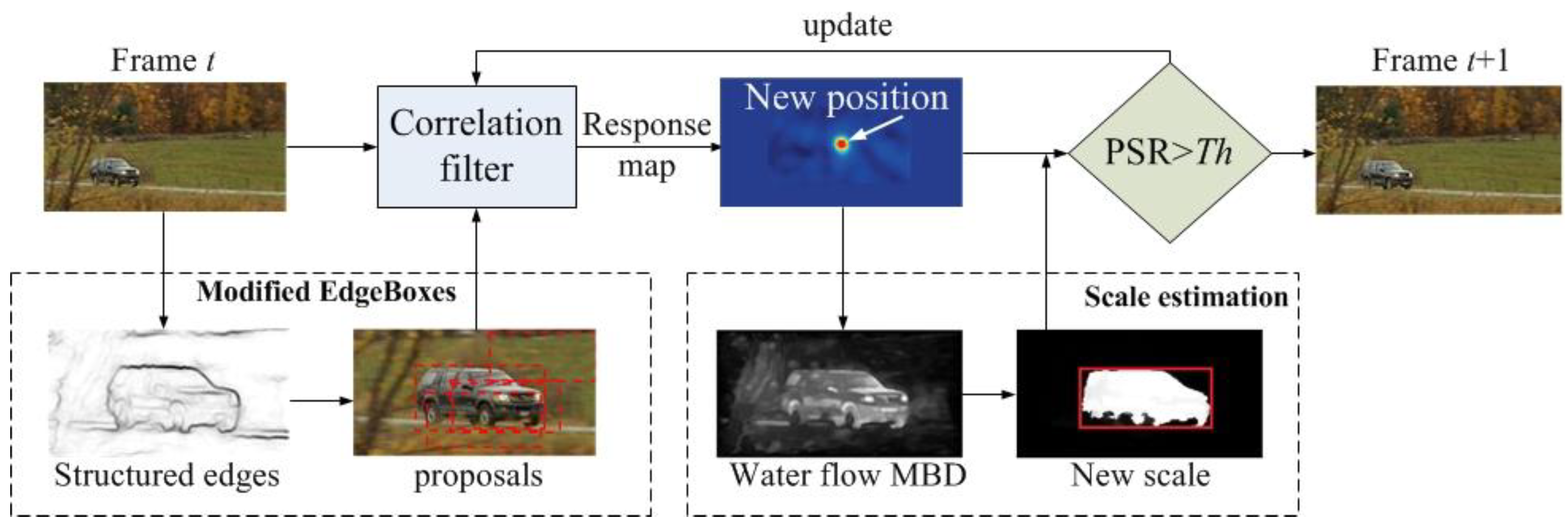
In this section, we describe the CFSA tracker in detail. The overview of the tracker is shown in Figure 1. The CFSA tracker mainly consists of four steps, namely, generating candidate proposals with modified EdgeBoxes, estimating the position of target object with kernelized correlation filter based tracking algorithm, scale estimation and updating schema. All the above steps will be described in details in the following subsections.

Figure 1.
Illustration of the proposed Correlation Filters based Scale Adaptive tracking method.
3.2. Generating Candidate Proposals with Modified EdgeBoxes
To improve the computational efficiency of object detection, several proposal generators were proposed recently, such as BING [37] and EdgeBoxes [26]. Compared with other existing proposal generators, EdgeBoxes has the advantages of high computational efficiency, high quality of proposals, and flexible parameter setting without training. All these advantages make it the most suitable proposal generator in a tracking algorithm. However, most of the generated proposals with high scores are large images or nearly the whole image. We modify the scoring metric of the EdgeBoxes generator, in which the closer the scale of the generated candidate object proposals to the tracked object, the higher the score. Given an image patch I, the generation of object proposals for tracking using the modified EdgeBoxes generator mainly includes five steps, namely, getting edges and edge groups, computing affinities of edge groups, computing weights of edge groups, computing scores of bounding boxes, and refining and ranking all bounding boxes. The detailed descriptions are as follows.
For each pixel in an image, EdgeBoxes initially compute an edge response with the structured edge detector [41] that has shown good performance and efficiency in predicting object boundaries. Then, edge groups are formed by combining 8 connected edges until the sum of their orientation differences is above a threshold (π/2). Small edge groups are merged with neighboring groups. Given a set of edge groups , the affinity of a pair of groups and is computed using:
where and are mean orientations of edge group and , respectively, is the angle between the mean position of group and the mean position of group . The value of may be used to adjust the affinity’s sensitivity to changes in orientation, with used in the literature.
The object proposal score of a candidate bounding box b can be calculated according to the set of edge groups G and their affinities. In this paper, we propose to calculate the bounding box score by combining the scale of target object to be tracked:
where each i corresponds to a pixel within the bounding box b, denotes the sum of the magnitudes for all edges in the group , and is the magnitude of edges p. denotes the central part of b, whose size is , while and are the width and height of b, respectively. is used to offset the bias of larger windows having more edges on average. is the arithmetic square root of the scale of the target object, which is used to offset the bias of large scale variations. For an image sequence, the above-mentioned target object is either the ground truth in the initial frame or the estimated target object in previous frame. The value of is used to control the speed at which the score decays with the scale of target object to be tracked. is a continuous value in [0, 1] that indicates whether is wholly contained in the bounding box b, which can be defined as:
where T is an ordered path of edge groups with a length of that begins with some and ends at . The higher value of means higher weight of edge group.
A sliding window search is performed on the whole image to find out all bounding box positions with a score above a given threshold, and then all candidate bounding boxes are refined using a greedy iterative search strategy. Finally the refined object proposals are filtered by Non-Maximal suppression, where a box is removed if the intersection over union (IoU) is more than a threshold for a box with greater score, and the ranked object proposals are identified.
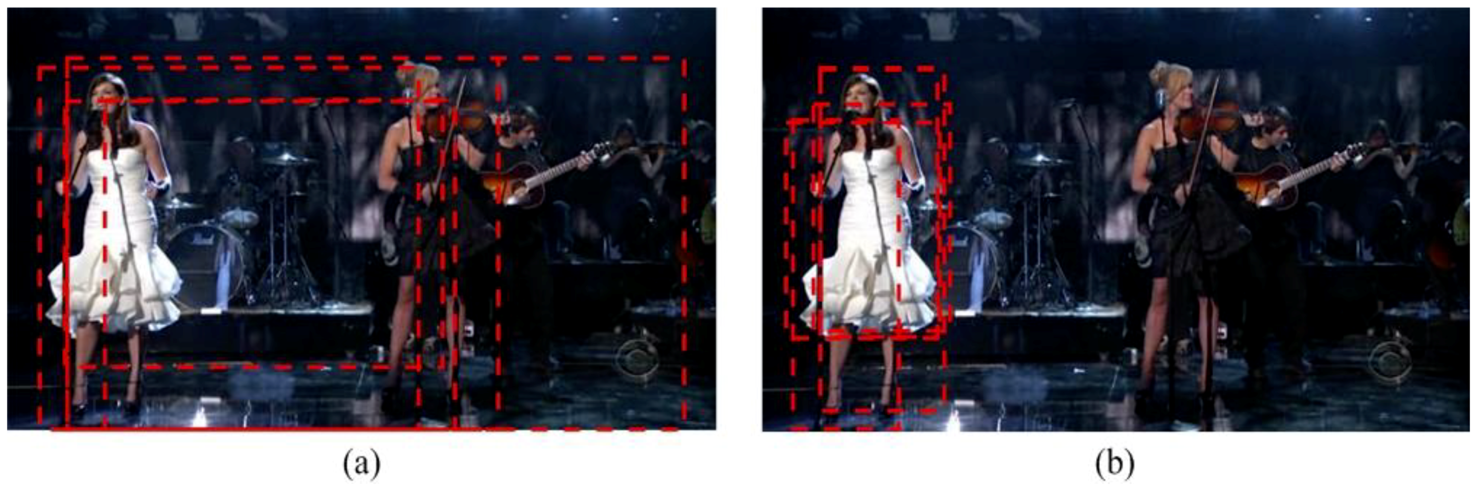
The runtime for the modified EdgeBoxes generator is mainly used in the detection of initial edges and the generation and refinement of proposals. The modified EdgeBoxes generator is carried out on an image that is twice the size of the estimated target object scale. Through experiments, we notice that the modified EdgeBoxes generates around 50 proposals per frame. After these proposals are filtered by Non-Maximal suppression, around 10 proposals per frame averagely are preserved. Reduction of image size and number of generated proposals can improve efficiency that the modified EdgeBoxes generator takes an average of 20 ms to generate the most appropriate proposals. Top five object proposals generated by EdgeBoxes and modified EdgeBoxes are shown in Figure 2. We can observe that the modified EdgeBoxes generator is more accurate than the original method.

Figure 2.
Examples of object proposals on image sequence Singer 1. (a) Top five object proposals generated by EdgeBoxes. (b) Top five object proposals generated by modified EdgeBoxes.
3.3. Tracking with Kernelized Correlation Filter
The proposed CFSA tracker is based on KCF tracker proposed in [18]. In this subsection, we review the main idea of KCF tracker and integrate object proposals into KCF tracker. As a discriminative method, KCF trains a linear model to estimate the probability that the image patch z is the target being tracked by solving a ridge regression problem,
where w is the model parameter matrix, is an image patch of size , i {0, 1, …, W−1} {0, 1, …, H−1}, is the regression target and is a regularization parameter used to control over-fitting.
Mapping the inputs of the linear ridge regression to a non-linear feature space with kernel trick that is defined by the kernel gets the non-linear ridge regression, which can be resolved as and denotes the dot-products of and . The coefficient can be expressed as:
where is a general kernel correlation, is the complex-conjugate of , and is the Discrete Fourier Transform (DFT) of . The training label is a Gaussian function, which decays smoothly from the value of one for the centered target to zero for other shifted samples. In order to integrate multiple features, the tracker needs to support multiple channels. In the Fourier domain, this can be achieved by summing the result for each channel with linearity of the DFT. 31 gradient orientation bins for HOG variant and 11 dimensions color naming are concatenated into a vector . In this paper, we adopt Gaussian kernel , multichannel features and circulant matrix trick,
where denotes the inverse Discrete Fourier Transform (IDFT). The full kernel correlation can be computed in only time using only a few DFT and IDFT.
In the tracking stage, the size of interesting image patch is cropped as the same with , and all responses for candidate image patches are calculated by:
where denotes the target appearance to be learnt in the model. And the target position is detected by finding the coordinate at which has the maximum value.
Subsequently, candidate object proposals are integrated into KCF tracker to estimate the position of the target object. While initialing, the target ground truth of size centered at position is given in the initial frame of a video. During tracking, when a new frame indexed by t comes, the modified EdgeBoxes generator is implemented on a patch centered at of size . Here is a scaling factor, reasonably larger than 1, containing some context information. Then, top N candidate object proposals can be obtained and the center of the k-th candidate object proposal is . We can get the pool of candidate object proposals , where is the estimated target object in the previous frame. Finally, all candidate proposals are correlated with KCF trackers and the new object position in current frame is estimated by identifying the maximum value of all responses.
3.4. Scale Estimation
In the detection step, an ideal scale estimation approach should be robust to scale changes while being computationally efficient [42]. In order to deal with the scale variations, we proposed to use the water flow driven MBD algorithm [27] to detect object on an image patch centered at the estimated position of the target object. Then the scale is estimated using the detected object and the initial given ground truth.
The main ideal of the water flow driven MBD algorithm is inspired by the natural phenomena of the water flow. Given an image, we assume seed pixels S (such as image boundary) as source of water, the water will flow from source pixels to other pixels with different flow cost. The flow cost is measured by MBD [43], which is widely used distance transform to measure pixel or region’s connectivity to the image boundary. For one N channels image I, the MBD of pixel i can be calculated as:
where a path on image I is a sequence of pixels where consecutive pairs of pixels are adjacent, denotes the set of all paths connecting pixel t and seed pixels S and is one channel image. For a color image, the number of image channels N = 3 while N is set to 1 for a grey image.
The process of detecting object and identifying the bounding box with the water flow driven MBD algorithm is as follows. In the initial, source pixels are flooded while all other pixels are droughty. The initial flooded pixels i are as following:
where and denotes two auxiliary maps that are used to keep track of the maximum and the minimum values on current path for each pixel. Then, the water will firstly flow to the droughty pixel which is neighboring to flooded pixels with the lowest cost, and then this droughty pixel becomes a flooded pixel. For each neighbor droughty pixel d of source pixel i, the flow from i to d can be estimated as:
Furthermore, the flow process continues until all pixels are flooded and the flooded image can be defined as:
As the target object always locates as the center of the image, all pixels of the image are emphasized according to its position. Moreover, post-processing including global smoothing filter, enhancement, and morphological smoothing are used to identify the object. The color image with the detected object is converted into grey image and a binary image is obtained with intensity using:
where iv denotes the intensity value of a pixel and is set to 150. Finally the bounding box is obtained, which compactly contains all pixels that the value of each pixel is 1 in the binary image . The water flow driven MBD algorithm only visit the image once, the post-processing and identifying bounding box of the detected object are all time-saving, the proposed method only needs about 6 ms to estimate the location and scale of an object in color image with the maximum dimension of 300 pixels. Due to the runtime and the interference in the image will increase with the increase of the dimension of the image, and the scale of the target object changes small in two consecutive frames, the scaling factor of the input image for scale estimation is set to 2 in this paper.
In the initial frame, the object is detected by the water flow driven MBD algorithm. If the scale of the detected object is the same as the scale of the ground truth, the estimated scale of target object to be tracked is the scale of detected object in subsequent frames. Otherwise, we compute the change in the scale as follows:
where is the position of the tracked object and is the position of the detected object bounding box in frame t. and are the estimated scale factor in frame t and t-1, respectively. We store all these scaling factors starting from the initial frame while changing the filter sizes, we use the mean of n scaling factors rather than the scaling factor estimated at the current frame.
3.5. Updating Schema
During tracking, it is important to adaptively updating correlation filters, because the target object’s appearance may undergo significant changes such as occlusion, background clutter, rotation and deformation. So, we train the new filter () at the newly estimated target location by linearly interpolating the newly estimated filter coefficients and the object appearance features with the ones in frame t − 1 only if the PSR of the maximum response in frame t is bigger than the given threshold Th, otherwise we keep the previous filters:
where is the learning rate, which determines how fast the tracker adapts itself to the changes in the scenes. r is the maximum response of the candidate proposals in frame t and Th is a given threshold of PSR that is used to determine whether the correlation filter is updated. As a confidence metric, the PSR is adopted to predict the tracking quality and estimate the reliability of a patch, which is widely used in signal processing to measure the signal peak strength in a correlation filter response map. A higher PSR value indicates that the estimated target object is more accurate. A smaller Th may add more background information into the new filter while a higher Th is not able to cope with appearance variations of the target object, which can lead to tracking failures. As we can see, the update schema is stopped to reduce the impact of the surrounding background when PSR of the estimated target object is smaller than the given threshold Th. Finally, the overall CFSA tracker is summarized into Algorithm 1.
| Algorithm 1. The proposed CFSA tracker. |
| Input: Previous target position ; target object model and ; frame Ft Output: Estimated position and scale of the target; Updated target object model and ; 1: if the initial frame then 2: Perform water flow driven MBD algorithm to detect object and determine scales in subsequent frames t are Equation (13) or the size of ; 3: end if 4: Generate object proposals with Equation (2) and get the pool of candidate object proposals ; 5: for each candidate object proposals do 6: Perform KCF tracker on its position using Equation (7); 7: end for 8: Estimate target position by maximizing all responses; 9: Perform water flow driven MBD algorithm to detect object on image patch centered at using Equations (8) to (12); 10: Estimate the target scale using Equation (13) or the size of ; 11: update the target model with Equations (14) and (15); |
4. Experiments
4.1. Experimental Configuration
Implementation details: The CFSA tracker is implemented in MATLAB on a regular PC with Intel i5-2450M CPU (2.50 GHz) processor, 4 GB memory and Debian 7.3 Operating System. In the proposed tracker, most of parameters are the same as the EdgeBoxes generator and the KCF tracker, the details are as follows. In the modified EdgeBoxes generator, the number of object proposals N is set to 5, the minimum box area of the object proposal is set to 0.7 times that of the target, is set to 30 to control the speed that the score decays with the target scale, and the threshold of IoU is set to 0.7. is set to 2 so that the modified EdgeBoxes generator can be performed on an image patch larger than the target. The learning rate and the Gaussian kernel parameter are set to 0.5 and 0.01, respectively. 11-channel color naming and 31-channel HoG features are used in our experiments, the size and the orientation number of HoG are 44 and 9, respectively. The searching window used to train the discriminative correlation filter should be larger than the given target so that the size of searching window is set to 2.5 times that of the target. The threshold Th that is used to determine whether the model is updated is set to 10 according to [15]. To estimate the scale of the target object, the mean of five scaling factors are used so that n is set to 4. All the above mentioned parameters are fixed throughout the experiments.
Benchmark dataset: In this section, experiments are performed on two frequently used public benchmark datasets OOTB [18,19,20,21] and OTB-100 [21,25] to evaluate the efficacy of the CFSA tracker. These challenging sequences are classified into 11 attributes [2,4], including deformation (DEF), occlusion (OCC), fast motion (FM), in-plane rotation (IPR), illumination variation (IV), out-of-view (OV), background clutters (BC), out-of-plane rotation (OPR), low resolution (LR), motion blur (MB), and scale variation (SV). One sequence may be annotated with many attributes, and some attributes occur more frequently than others, for example, OPR and IPR. The position and scale of the target are given in the ground truth of benchmark datasets for initialization and evaluation. Please refer to OOTB [2] and OTB-100 [4] datasets for more details.
Evaluation methodology: In this paper, the results of one-pass evaluation (OPE) are shown. OPE means running the tracking algorithm throughout a test sequence with initialization from the ground truth position in the first frame and reporting the average precision and success rate [2]. The precision and success rate are two widely used evaluation metrics for quantitative analysis [2,4]. The precision plot refers to the center location error (CLE), which is defined as the average Euclidean distance between the center locations of the tracked target object and the manually labeled ground truths. The success plot is defined as the bounding box overlap, and the overlap score can be computed with , where denotes the bounding box of tracked result, denotes the bounding box of ground truth, | · | is the number of pixels of the regions, and and represent the intersection and union of two regions.
4.2. Quantitative Comparisons
4.2.1. Overall Performance
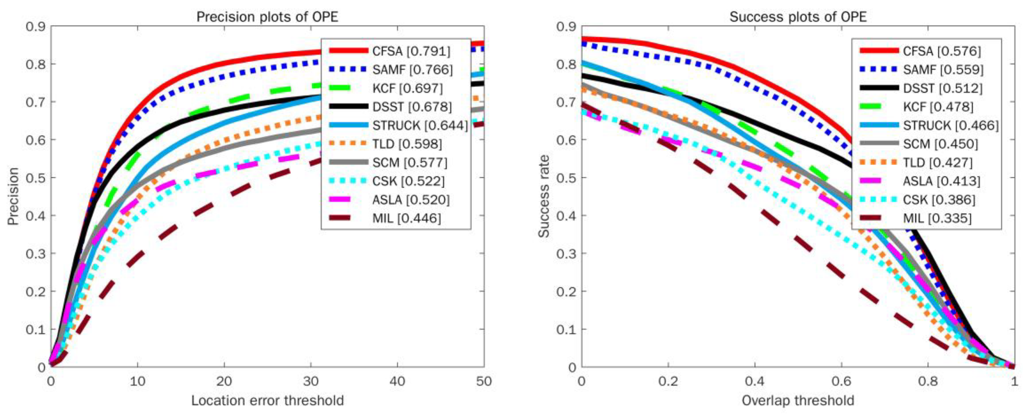
The CFSA tracker has been quantitatively compared with 9 state-of-the-art trackers and codes of these trackers are publicly available, including CSK [16], KCF [18], TLD [44], SAMF [28], Struck [13], MIL [12], ASLA [45], SCM [46], and DSST [22]. In these trackers, CSK, KCF, SAMF, and DSST are correlation filter based trackers, and TLD, Struck, MIL, ASLA and SCM are representative trackers using single or multiple online classifiers. Moreover, SAMF and DSST trackers pay more attention on the estimation of the target scale. The quantitative comparison results of OPE on OOTB dataset and OTB-100 dataset are shown in Figure 3 and Figure 4, respectively. For success plots, the values in square brackets indicate the area under curve (AUC) value. For precision plots, the values in square brackets represent the scores at error threshold of 20 pixels. It can be observed that the CFSA tracker performs favorably against other state-of-the-art and competitive trackers. Compared to the original KCF, the CFSA tracker outperforms KCF on the OOTB dataset by 13% in the precision plot and 8.3% in the success plot, respectively. Moreover, the CFSA outperforms both DSST and SAMF on the OTB-100 dataset, giving 6.4% and 1.7% better overlap scores.
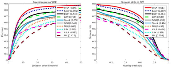
Figure 3.
Precision and success plots over OOTB benchmark dataset using one-pass evaluation.
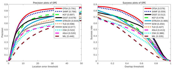
Figure 4.
Precision and success plots over OTB-100 benchmark dataset using OPE.
4.2.2. Robustness Evaluation
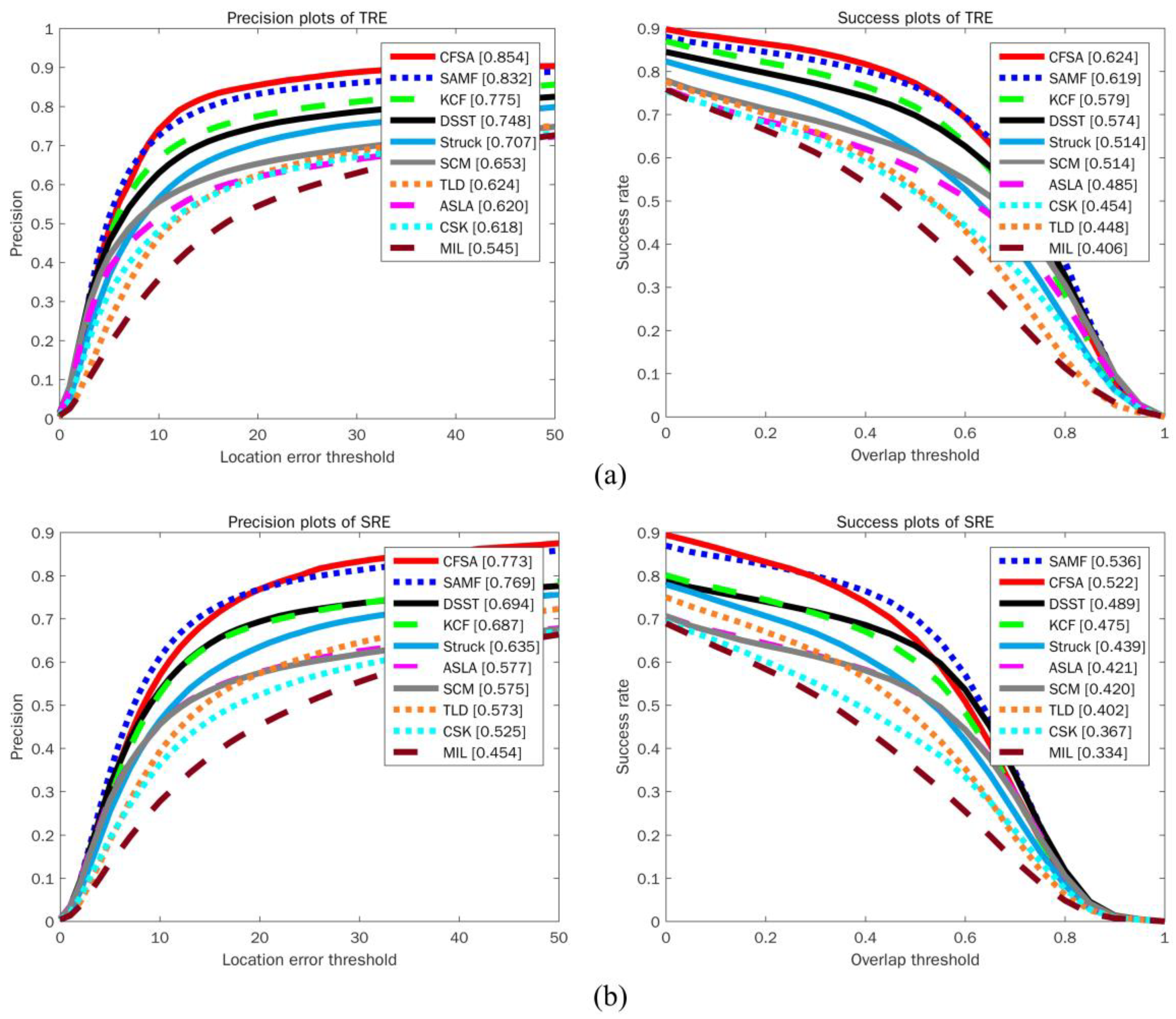
Spacial robustness evaluation (SRE) and temporal robustness evaluation (TRE) [2] are commonly utilized to evaluate the robustness of a tracker. SRE evaluates the robustness of a tracker with different bounding boxes by shifting or scaling the ground-truth in the initial frame, while TRE evaluates the robustness of a tracker with different initialization at a different start frame. The experimental results of robustness evaluation are shown in Figure 5. It can be seen from the figure that the CFSA tracker performs better than other trackers in terms of different evaluation metrics. In the precision plots, SAMF and KCF achieve the best performance among these state-of-the-art trackers, while CFSA tracker outperforms SAMF and KCF with better scores of 85.4% in TRE and 77.3% in SRE.
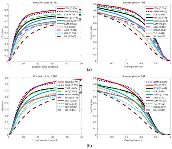
Figure 5.
Precision and success plots over OOTB benchmark dataset using (a) temporal robustness evaluation and (b) spacial robustness evaluation. The performance score for each tracker is shown in the legend.
4.2.3. Attribute-Based Performance
To thoroughly evaluate the performance of the CFSA tracker under various challenging scenarios, we analyze the performance based on the above-mentioned 11 different attributes on OOTB and OTB-100 datasets. Table 1 and Table 2 show the precision scores on the OOTB dataset at the center location error threshold = 20 pixels and the success scores of AUC, respectively. The results on the OTB-100 dataset are shown in Table 3 and Table 4. The row headers indicate the attributes and its number of image sequences. As shown in these tables, CFSA tracker performs better than other trackers in 9 of 11 attributes and the CFSA tracker exhibits significant improvements in handing scale variation, deformation and in-plane and out-of-plane rotation. Compared with the SAMF tracker which estimates target scale on multiple resolutions of the searching area and achieves prior performance, the performance of CFSA tracker on OOTB dataset outperforms SAMF by 1.8% in the precision plot and 2.5% in the success plot in handing scale variations. This is mainly benefit from the usage of water flow driven MBD algorithm and the proposed scale estimation method, which improved the accuracy of estimated scale of the target object. Moreover, we can observe that the CFSA tracker can well deal with deformation and rotation in two benchmark datasets. This is mainly due to the generated candidate proposals are based on the grouped edge information in an image and the HOG and color naming features are invariant to local small deformation and rotation. However, as shown in Table 2, the SAMF tracker performs better than the proposed CFSA tracker in the case of background clutter, the main reason might be that the tracking performance decreases as the difficulty of generating high-quality proposals and estimating the scale of the target object increases.

Table 1.
The precision scores of CFSA tracker and nine other trackers at the center location error threshold = 20 pixels on the OOTB dataset. Bold and underline values indicate best and second performances, respectively.

Table 2.
The success plot’s area under curve scores of CFSA tracker and nine other state-of-the-art trackers on the OOTB dataset. Bold and underline values indicate best and second performances, respectively.

Table 3.
The precision scores of CFSA tracker and nine other trackers at the center location error threshold = 20 pixels on the OTB-100 dataset. Bold and underline values indicate best and second performances, respectively.

Table 4.
The success plot’s AUC scores of CFSA tracker and nine other state-of-the-art trackers on the OTB-100 dataset. Bold and underline values indicate best and second performances, respectively.
4.2.4. Components Analysis
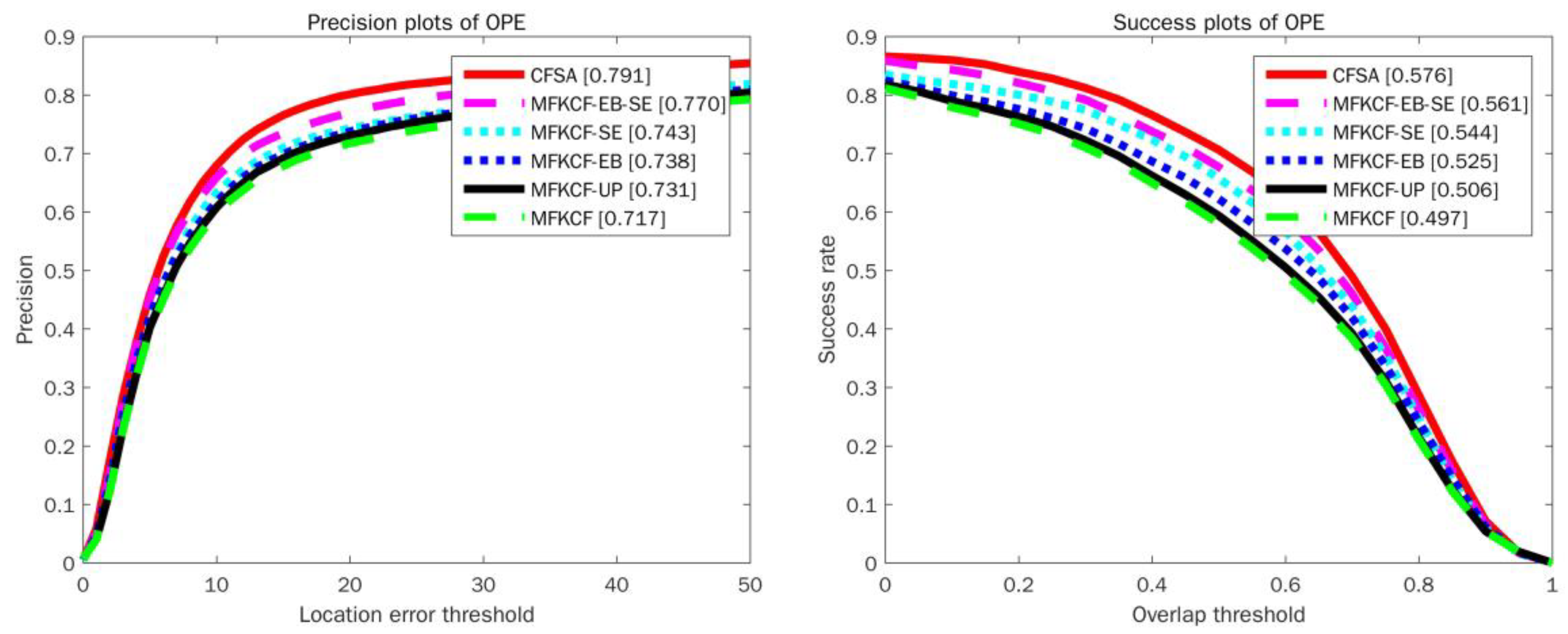
The CFSA tracker consists of three modules: the modified EdgeBoxes (EB), the water flow driven MBD based scale estimation (SE) and PSR based model updating (UP). The CFSA tracker is compared with five other trackers, which are implemented by combining one of the components with multiply features (HOG and color naming) based KCF tracker, including multiply features based KCF tracker MFKCF, EB based tracker MFKCF-EB, SE based tracker MFKCF-SE, UP based tracker MFKCF-UP and EB and SE based tracker MFKCF-EB-SE. These trackers are evaluated on the OTB-100 dataset with OPE. The contribution of each component to the performance of the CFSA tracker is shown in Figure 6. We can observe that the trackers MFKCF-EB, MFKCF-SE, and MFKCF-UP all show a significant drop in both the precision plots and the success plots compared to the CFSA tracker. However, the MFKCF-EB-SE tracker, which combines EB and SE, greatly improves the overall performance of the MFKCF tracker, mainly due to the complementary of each component. Specifically, the EBT tracker tracks the target object with re-ranked high-quality proposals generated by the EdgeBoxes component and achieves promising results on OOTB dataset with 84.8% in the precision plot and 58.1% in the success plot. The EBT tracker outperforms CFSA tracker by 0.7% in the precision plot while the CFSA tracker outperforms EBT tracker by 3.6% in the success plot. This mainly benefits from the combination of locating target object with high-quality proposals based correlation filters and estimating target scale with the proposed scale estimation method.
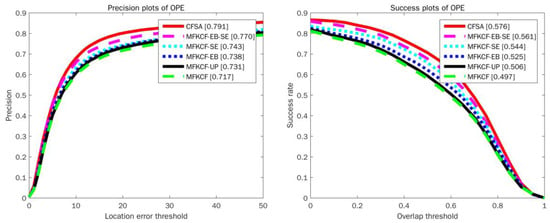
Figure 6.
Comparison of three components. Precision and success plots on OTB-100 benchmark dataset using OPE are shown.
4.2.5. Speed Analysis
The major computational cost of the CFSA tracker is the generation of candidate proposals and estimation of object position, the speed of the proposed method is about 18.5 fps without code optimization. The speeds of other trackers are shown in Table 5. We can observe that CSK tracker is faster than all of other trackers with the running speed of 269 fps. The CFSA tracker ranks 6th among all trackers and 4th in correlation filter based trackers. Compared with other correlation filter based trackers, CFSA tracker achieves a balance between running speed and tracking performance and can be extended to a parallel implementation to optimize its efficiency.

Table 5.
The running speed of CFSA and other state-of-the-art trackers on OOTB benchmark dataset. Bold and underline values indicate best and second running speed, respectively. fps: frames per second.
4.2.6. Parameter Sensitivity Analysis
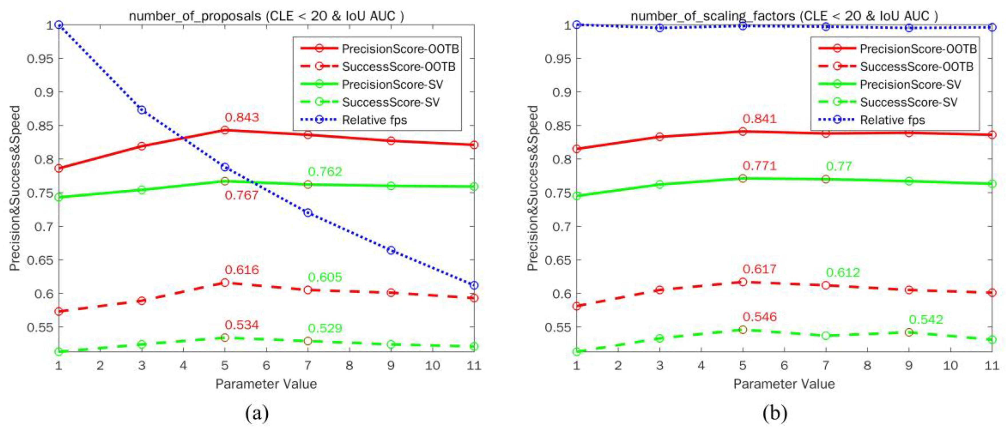
In the proposed tracker, some parameters are hard to decide via theoretical derivation, thus their settings are mainly empirical. To investigate the effects of these parameters, we moderately traverse their possible settings and perform a parameter sensitivity analysis. Each parameter is examined individually on the OOTB dataset and its subset (scale variation), while the other parameter settings remain the same as the original setup in CFSA tracker. The tracking accuracy of OPE (precision and success rate) and speed in the form of relative fps normalized to the highest one are reported in Figure 7.
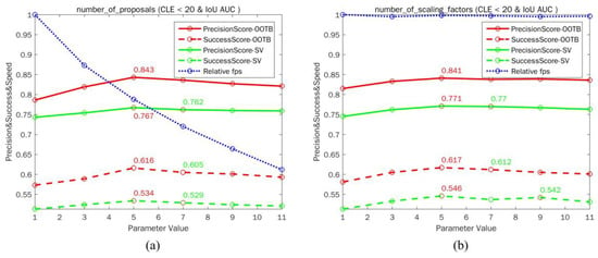
Figure 7.
The tracking accuracy and speed under different settings of parameters: (a) the number of proposals N (b) the number of scaling factors n. In the legend, precision and success plots on OOTB dataset and its subset (scale variation) using OPE are shown, and relative fps is collected on the OOTB dataset. The values of highest and the second highest accuracies are shown in red and green respectively.
The results of CFSA tracker with different number of proposals are shown in Figure 7a and we can observe that as the number of proposals increases, the performance of CFSA tracker increases first and then decreases. The main reason might be that more accurate proposals could help to estimate the position of the target, while more inaccurate proposals might add more background information that leads to tracking failures. However, with the increase in the number of proposals, tracking speed is getting slower and slower. Thus the number of proposals 5 should be the most promising. In Figure 7b, the number of scaling factors n for estimating the scale of the target object is investigated. We can observe that the performance of CFSA tracker can be improved by averaging several scaling factors of consecutive frames and the number of scaling factors has almost no effect on tracking speed.
4.3. Qualitative Comparisons
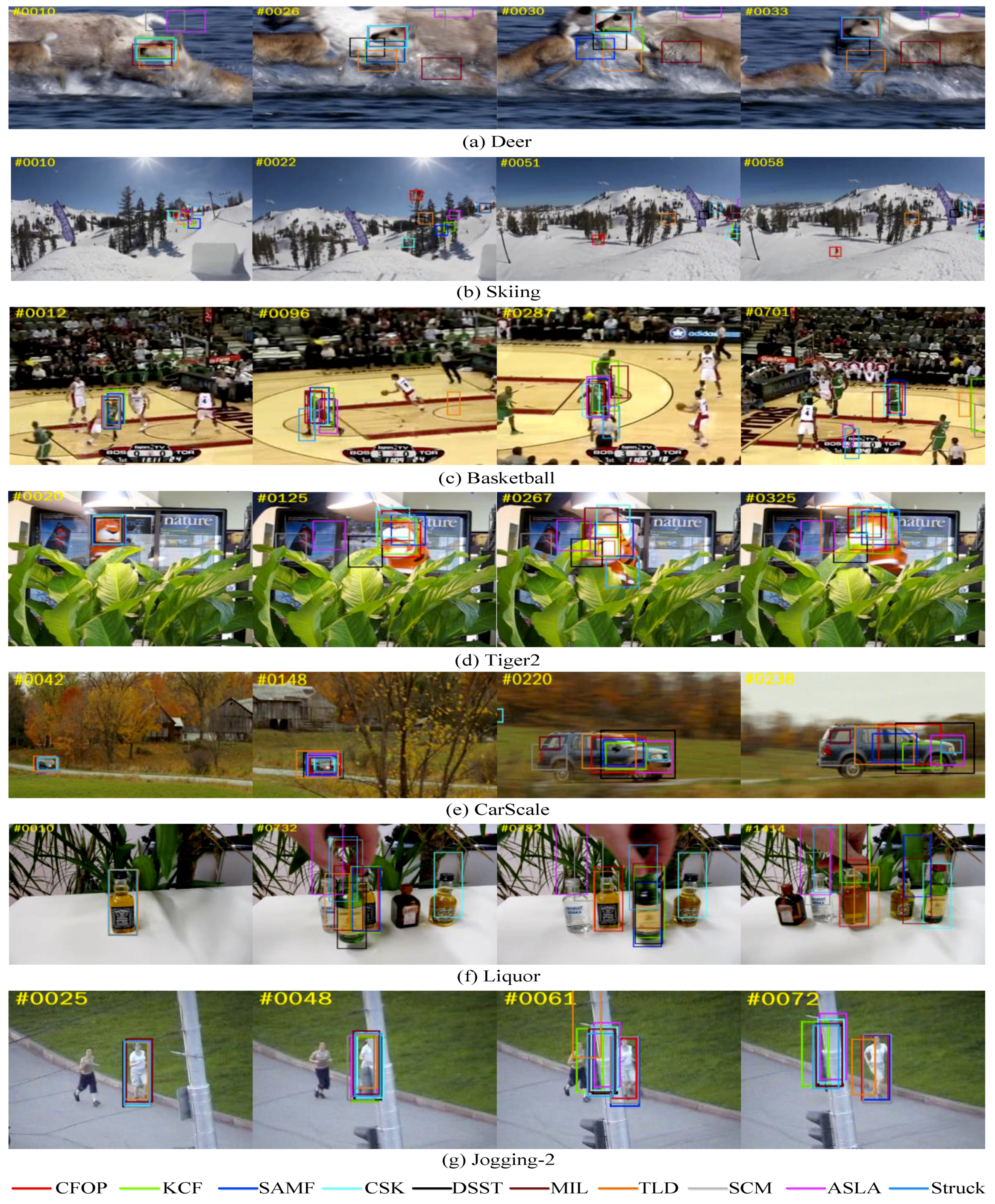
In this subsection, the proposed CFSA tracker is qualitatively compared with 9 state-of-the-art trackers and tracking results of 7 representative image sequences with all 11 attributes are shown in Figure 8. In the following, we compare the tracking results of these trackers when the target object undergoes rotation, deformation, scale variation and occlusion.
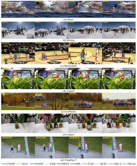
Figure 8.
Compared qualitative results of CFSA tracker with nine other trackers on seven challenging sequences, i.e., (a) Deer, (b) Skiing, (c) Basketball, (d) Tiger2, (e) CarScale, (f) Liquor and (g) Jogging-2 sequence.
(1) Rotation: Rotation is a type of challenging appearance changes that occurs frequently, mainly divided into in-plane rotation and out-of-plane rotation. Figure 8a,b show the tracking results on two challenging sequences to evaluate whether CFSA tracker is able to deal with rotation. In the Deer sequence, SCM and ASLA start drifting at frame 10 due to the in-plane rotation of the target. At frame 26, 30 and 33, all trackers except CFSA, CSK, SAMF and Struck drift to the background. Due to the fast motion and continuous rotation of the target, all trackers apart from CFSA are failed to track the target in the Skiing sequence (e.g., #0021, #0051 and #0058). Moreover, as shown in Figure 8e, the target liquor bottle is fast moving with out-of-plane rotation at frame 1414, only CFSA could accurately track the target.
(2) Deformation: Figure 8c,d are used to qualitatively assess each tracker in the aspect of handling deformation. The tracking results as presented in the Basketball sequence show that CFSA, CSK and SAMF could track the target object on most of the entire sequence, while other trackers fail to track the target or drift away from the target object at frame 96, 287 and 701. The sequence of Tiger2 contains challenging factors such as fast motion, partially occlusion, in-plane rotation, out-of-plane rotation and deformation. For example, the tiger opens his mouth at frame 125 and is partially occluded at frame 267, resulting in most of the trackers cannot accurately locate the target and estimate its target scale, while the KCF and CFSA trackers could stick to the target in the whole sequence.
(3) Scale variation: In order to prove the effectiveness of the CFSA tracker in the case of significant scale variation, Figure 8e shows the tracking results of CarScale sequence. The car is far away and its scale changes little at frame 42, all trackers could stick to the car. As the car approaches, its scale changes rapidly, most trackers can successfully track the car, but the bounding box does not change with the scale of the car at frame 148 and 220. TLD, DSST, and CFSA perform better than other trackers at frame 220 and 238. Compared with CFSA tracker, the DSST tracker is faster. This is mainly due to too much time (about 26 ms per frame on average) is spent on the generation of high-quality proposals and the detection of the target car’s position, while these two parts are critical for estimating the position and scale of the target object. After getting the accurate position of the target car, its scale can be estimated in 6ms. However, CFSA and all other state-of-the-art trackers cannot accurately estimate the scale of the target object when the scale changes quickly, which should be noted in future studies. Furthermore, in Figure 8f, the target bottle is rotated and its scale changed at frame 1414. Only CFSA could accurately track the target bottle and estimate its size. Benefit from the water flow driven MBD algorithm and scale estimation method, the CFSA tracker is able to track the target and estimate its scale more accurate.
(4) Occlusion: The target object may be partially or heavily occluded as shown in Figure 8f,g. For the Liquor sequence, all trackers can successfully track the target bottle at frame 10, and then all trackers except KCF and CFSA have already lost the target when the target bottle is occluded by another green bottle at frame 732 and reappears at frame 782. In the sequence of Jogging-2, the running woman is occluded by a traffic signal pole at frame 48 and 61 and reappears at frame 72. All trackers except SCM, SAMF and CFSA drift to the traffic signal pole and only the TLD tracker redetected the woman in subsequent frames. The reason why the proposed CFSA tracker handles occlusion well can be attributed to the usage of updating schema and high-quality proposals generated by the modified EdgeBoxes generator.
Although the performance of the CFSA tracker has been improved significantly under various challenging scenarios, the performance in handling background clutter and occlusion can be further improved compared with the BACF tracker [47] proposed by Galoogahii. Moreover, when the appearance of the target object or the scene changes quickly [20,48], the tracker may fail to track the target object. In the future research, we will try to integrate the background and context information into the tracker to deal with these challenges.
5. Conclusions
In this paper, we propose a correlation filter based scale adaptive visual tracker. In the proposed CFSA tracker, the modified EdgeBoxes generator could obtain higher quality candidate object proposals for tracking than other existing detection proposal generators. By integrating these candidate proposals into a KCF tracker and tracking with HOG and color naming features, the proposed tracker can achieve better performance on various challenging scenarios such as occlusion, rotation and deformation. Moreover, the proposed scale estimation method based on water flow driven MBD algorithm further improves its robustness to scale variations. The updating schema with PSR could reduce the introduction of surrounding background and alleviate the drifting problem. Experimental results on OOTB and OTB-100 benchmark datasets demonstrate that the CFSA tracker achieves a near real time tracking with better performance than several state-of-the-art trackers.
Author Contributions
C.L. designed the algorithm, performed the experiments and wrote the paper. B.Y. supervised the research and improved the paper.
Funding
This research received no external funding.
Conflicts of Interest
The authors declare no conflict of interest.
References
- Li, X.; Hu, W.; Shen, C.; Zhang, C.; Zhang, Z.; Dick, A.; Hengel, A.V.D. A survey of appearance models in visual object tracking. ACM Trans. Intell. Syst. Technol. 2013, 4, 1–42. [Google Scholar] [CrossRef]
- Wu, Y.; Lim, J.; Yang, M.H. Online object tracking: A benchmark. In Proceedings of the IEEE Conference on Computer Vision and Pattern Recognition (CVPR), Portland, OR, USA, 23–28 June 2013; pp. 2411–2418. [Google Scholar]
- Smeulders, A.W.M.; Chu, D.M.; Cucchiara, R.; Calderara, S.; Dehghan, A.; Shah, M. Visual tracking: An experimental survey. IEEE Trans. Pattern Anal. Mach. Intell. 2014, 36, 1442–1468. [Google Scholar] [PubMed]
- Wu, Y.; Lim, J.; Yang, M.H. Object tracking benchmark. IEEE Trans. Pattern Anal. Mach. Intell. 2015, 37, 1834–1848. [Google Scholar] [CrossRef] [PubMed]
- Zhang, L.; Suganthan, P.N. Robust visual tracking via co-trained kernelized correlation filters. Pattern Recognit. 2017, 69, 82–93. [Google Scholar] [CrossRef]
- Huang, Z.; Ji, Y. Robust and efficient visual tracking under illumination changes based on maximum color difference histogram and min-max-ratio metric. J. Electron. Imaging 2013, 22, 6931–6946. [Google Scholar]
- Jeong, S.; Paik, J. Partial Block Scheme and Adaptive Update Model for Kernelized Correlation Filters-Based Object Tracking. Appl. Sci. 2018, 8, 1349. [Google Scholar] [CrossRef]
- Hu, Z.; Xie, R.; Wang, M.; Sun, Z. Midlevel cues mean shift visual tracking algorithm based on target-background saliency confidence map. Multimed. Tools Appl. 2017, 1, 21265–21280. [Google Scholar] [CrossRef]
- Ross, D.A.; Lim, J.; Lin, R.S.; Yang, M.H. Incremental learning for robust visual tracking. Int. J. Comput. Vis. 2008, 77, 125–141. [Google Scholar] [CrossRef]
- Zhong, W.; Lu, H.; Yang, M.H. Robust object tracking via sparsity-based collaborative model. In Proceedings of the IEEE Conference on Computer Vision and Pattern Recognition (CVPR), Providence, RI, USA, 16–21 June 2012; pp. 1838–1845. [Google Scholar]
- Jia, X.; Lu, H.; Yang, M.H. Visual tracking via coarse and fine structural local sparse appearance models. IEEE Trans. Image Process. 2016, 25, 4555–4564. [Google Scholar] [CrossRef] [PubMed]
- Babenko, B.; Yang, M.H.; Belongie, S. Robust object tracking with online multiple instance learning. IEEE Trans. Pattern Anal. Mach. Intell. 2011, 33, 1619–1632. [Google Scholar] [CrossRef] [PubMed]
- Hare, S.; Golodetz, S.; Saffari, A.; Vineet, V.; Cheng, M.M.; Hicks, S.L.; Torr, P.H. Struck: Structured output tracking with kernels. IEEE Trans. Pattern Anal. Mach. Intell. 2016, 38, 2096–2109. [Google Scholar] [CrossRef] [PubMed]
- Chen, S.; Zhu, S.; Yan, Y. Robust visual tracking via online semi-supervised co-boosting. Multimed. Syst. 2016, 22, 297–313. [Google Scholar] [CrossRef]
- Bolme, D.S.; Beveridge, J.R.; Draper, B.A.; Lui, Y.M. Visual object tracking using adaptive correlation filters. In Proceedings of the IEEE Conference on Computer Vision and Pattern Recognition (CVPR), San Francisco, CA, USA, 13–18 June 2010; pp. 2544–2550. [Google Scholar]
- Henriques, J.F.; Caseiro, R.; Martins, P.; Batista, J. Exploiting the circulant structure of tracking-by-detection with kernels. In Proceedings of the European Conference on Computer Vision (ECCV), Florence, Italy, 7–13 October 2012; pp. 702–715. [Google Scholar]
- Danelljan, M.; Khan, F.S.; Felsberg, M.; Weijer, J.V.D. Adaptive color attributes for real-time visual tracking. In Proceedings of the IEEE Conference on Computer Vision and Pattern Recognition (CVPR), Columbus, OH, USA, 23–28 June 2014; pp. 1090–1097. [Google Scholar]
- Henriques, J.F.; Caseiro, R.; Martins, P.; Batista, J. High-speed tracking with kernelized correlation filters. IEEE Trans. Pattern Anal. Mach. Intell. 2015, 37, 583–596. [Google Scholar] [CrossRef] [PubMed]
- Chen, K.; Tao, W.; Han, S. Visual object tracking via enhanced structural correlation filter. Inf. Sci. 2017, 394, 232–245. [Google Scholar] [CrossRef]
- Ma, C.; Huang, J.B.; Yang, X.; Yang, M.H. Adaptive correlation filters with long-term and short-term memory for object tracking. Int. J. Comput. Vis. 2018, 126, 771–796. [Google Scholar] [CrossRef]
- Zhang, X.; Xia, G.S.; Lu, Q.; Shen, W.; Zhang, L. Visual object tracking by correlation filters and online learning. ISPRS J. Photogr. Remote Sens. 2017, 140, 77–89. [Google Scholar] [CrossRef]
- Danelljan, M.; Häger, G.; Khan, F.S. Accurate scale estimation for robust visual tracking. In Proceedings of the British Machine Vision Conference (BMVC), Nottingham, UK, 1–5 September 2014; pp. 65.1–65.11. [Google Scholar]
- Bai, B.; Zhong, B.; Ouyang, G.; Wang, P.; Liu, X.; Chen, Z.; Wang, C. Kernel correlation filters for visual tracking with adaptive fusion of heterogeneous cues. Neurocomputing 2018, 286, 109–120. [Google Scholar] [CrossRef]
- Liu, T.; Wang, G.; Yang, Q. Real-time part-based visual tracking via adaptive correlation filters. In Proceedings of the IEEE Conference on Computer Vision and Pattern Recognition (CVPR), Boston, MA, USA, 7–12 June 2015; pp. 4902–4912. [Google Scholar]
- Yang, L.; Jiang, P.; Wang, F.; Wang, X. Robust real-time visual object tracking via multi-scale fully convolutional Siamese networks. Multimed. Tools Appl. 2018, 77, 22131–22143. [Google Scholar] [CrossRef]
- Zitnick, C.L.; Dollar, P. Edge boxes: Locating object proposals from edges. In Proceedings of the European Conference on Computer Vision (ECCV), Zurich, Switzerland, 6–12 September 2014; pp. 391–405. [Google Scholar]
- Huang, X.; Zhang, Y. Water flow driven salient object detection at 180 fps. Pattern Recognit. 2018, 76, 95–107. [Google Scholar] [CrossRef]
- Li, Y.; Zhu, J. A scale adaptive kernel correlation filter tracker with feature integration. In Proceedings of the European Conference on Computer Vision (ECCV), Zurich, Switzerland, 6–12 September 2014; pp. 254–265. [Google Scholar]
- Rapuru, M.K.; Kakanuru, S.; Venugopal, P.M.; Mishra, D.; Subrahmanyam, G.R.K.S. Correlation based tracker level fusion for robust visual tracking. IEEE Trans. Image Process. 2017, 26, 4832–4842. [Google Scholar] [CrossRef] [PubMed]
- Carreira, J.; Sminchisescu, C. Constrained parametric min-cuts for automatic object segmentation. In Proceedings of the IEEE Conference on Computer Vision and Pattern Recognition (CVPR), San Francisco, CA, USA, 13–18 June 2010; pp. 3241–3248. [Google Scholar]
- Uijlings, J.R.R.; Van De Sande, K.E.A.; Gevers, T.; Smeulders, A.W.M. Selective search for object recognition. Int. J. Comput. Vis. 2013, 104, 154–171. [Google Scholar] [CrossRef]
- Cheng, M.M.; Zhang, Z.; Lin, W.Y.; Torr, P. BING: Binarized normed gradients for objectness estimation at 300 fps. In Proceedings of the IEEE Conference on Computer Vision and Pattern Recognition (CVPR), Columbus, OH, USA, 23–28 June 2014; pp. 3286–3293. [Google Scholar]
- Girshick, R.; Donahue, J.; Darrell, T.; Malik, J. Rich feature hierarchies for accurate object detection and semantic segmentation. In Proceedings of the IEEE Conference on Computer Vision and Pattern Recognition (CVPR), Columbus, OH, USA, 23–28 June 2014; pp. 580–587. [Google Scholar]
- Galteri, L.; Seidenari, L.; Bertini, M.; Bimbo, A.D. Spatio-temporal closed-loop object detection. IEEE Trans. Image Process. 2017, 26, 1253–1263. [Google Scholar] [CrossRef] [PubMed]
- Ke, W.; Chen, J.; Ye, Q. Deep contour and symmetry scored object proposal. Pattern Recognit. Lett. 2018, in press. [Google Scholar] [CrossRef]
- Zhu, G.; Porikli, F.; Li, H. Beyond local search: Tracking objects everywhere with instance-specific proposals. In Proceedings of the IEEE Conference on Computer Vision and Pattern Recognition (CVPR), Seattle, WA, USA, 27–30 June 2016; pp. 943–951. [Google Scholar]
- Liang, P.; Pang, Y.; Liao, C.; Mei, X.; Ling, H. Adaptive objectness for object tracking. IEEE Signal Process. Lett. 2016, 23, 949–953. [Google Scholar] [CrossRef]
- Kwon, J.; Lee, H. Visual tracking based on edge field with object proposal association. Image Vis. Comput. 2018, 69, 22–32. [Google Scholar] [CrossRef]
- Meshgi, K.; Mirzaei, M.S.; Oba, S. Information-maximizing sampling to promote tracking-by-detection. In Proceedings of the IEEE International Conference on Image Processing (ICIP), Athens, Greece, 7–10 October 2018; pp. 2700–2704. [Google Scholar]
- Huang, D.; Luo, L.; Chen, Z.; Wen, M.; Zhang, C. Applying detection proposals to visual tracking for scale and aspect ratio adaptability. Int. J. Comput. Vis. 2017, 122, 524–541. [Google Scholar] [CrossRef]
- Zitnick, C.L. Structured forests for fast edge detection. In Proceedings of the IEEE International Conference on Computer Vision (ICCV), Sydney, Australia, 1–8 December 2013; pp. 1841–1848. [Google Scholar]
- He, Z.; Fan, Y.; Zhuang, J.; Dong, Y.; Bai, H.L. Correlation filters with weighted convolution responses. In Proceedings of the IEEE International Conference on Computer Vision (ICCV), Venice, Italy, 22–29 October 2017; pp. 1992–2000. [Google Scholar]
- Strand, R.; Ciesielski, K.C.; Malmberg, F.; Saha, P.K. The minimum barrier distance. Comput. Vis. Image Underst. 2013, 117, 429–437. [Google Scholar] [CrossRef]
- Kalal, Z.; Mikolajczyk, K.; Matas, J. Tracking-learning-detection. IEEE Trans. Pattern Anal. Mach. Intell. 2012, 34, 1409–1422. [Google Scholar] [CrossRef] [PubMed]
- Jia, X. Visual tracking via adaptive structural local sparse appearance model. In Proceedings of the IEEE Conference on Computer Vision and Pattern Recognition (CVPR), Providence, RI, USA, 16–21 June 2012; pp. 1822–1829. [Google Scholar]
- Zhong, W.; Lu, H.; Yang, M.H. Robust object tracking via sparse collaborative appearance model. IEEE Trans. Image Process. 2014, 23, 2356–2368. [Google Scholar] [CrossRef] [PubMed]
- Galoogahi, H.K.; Fagg, A.; Lucey, S. Learning background-aware correlation filters for visual tracking. In Proceedings of the IEEE International Conference on Computer Vision (ICCV), Venice, Italy, 22–29 October 2017; pp. 1144–1152. [Google Scholar]
- Yang, M.; Wu, Y.; Hua, G. Context-aware visual tracking. IEEE Trans. Pattern Anal. Mach. Intell. 2009, 31, 1195–1209. [Google Scholar] [CrossRef] [PubMed]
© 2018 by the authors. Licensee MDPI, Basel, Switzerland. This article is an open access article distributed under the terms and conditions of the Creative Commons Attribution (CC BY) license (http://creativecommons.org/licenses/by/4.0/).

