A System for Analysing the Basketball Free Throw Trajectory Based on Particle Swarm Optimization

Abstract

This paper describes a system for the automatic detection and tracking of a ball trajectory during a free throw. The tracking method is based on a particle swarm optimization (PSO) algorithm. The proposed method allows for the measurement of selected parameters of a basketball free throw trajectory. Ten parameters (four distances, three velocities, and three angle parameters) were taken into account. The research material included 200 sequences captured by a 100 Hz monocular camera. The study was based on a group of 30 basketball players who played in the Polish Second Division during the 2015/2016 season and the Youth Polish National Team in 2017. The experimental results showed the differences between the parameters in both missed and hit throws. The proposed system may be used in the training process as a tool to improve the technique of the free throw in basketball.

1. Introduction

An important issue in sport is to analyse the factors that influence the achievement of the best sports results. In every sports discipline, there are elements whose performance has a direct impact on the final outcome. One such element in basketball includes the free throw which is very crucial in this kind of sport; therefore, it is essential to go through a scientific analysis to improve the free throw skills and hit rate of basketball players [1]. A free throw is a special component of the technical preparation of every player, which is based on automatic movement. It is always performed in the same way (with a suitable rhythm and speed).

A substantial body of research into the different aspects of basketball has been carried out to date [2,3,4,5,6]. These studies include research into the ways to improve a free throw. One example is the research conducted by Englert et al. [7] in which the scientists rated the levels of concentration of the player throwing free throws. In other studies, Hamilton and Reinschmidt [8] analysed the speed of the ball, the throw angle and the impact of those components on the effectiveness of a free throw. Button et al. [9], however, have evaluated the posture of a player during a free throw. Another paper [6] describes the analysis of selected kinematic parameters of free throws performed during the learning process, and identifies which one has the greater impact on the effectiveness of the throws. They used a 200 Hz camera and SIMI-Motion software (Simi Reality Motion Systems GmbH, Unterschleissheim, Germany). Gablonsky and Lang [3] presented a mathematical model of the free throw, which involves the initial angle, velocity and trajectory of the ball. This research has been explored further by Murphy [10]. The author focused on finding the best values for the parameters of a free throw. The player’s body height, and the angle and speed of the ball were all taken into consideration. A similar problem was considered by Tran and Silverberg [11], who analysed the initial angle, speed, rotation and height of the ball’s flight. An analysis presented by them showed that the angle of the ball during the throw should be about ${52}^{\circ }$, which allows for an effectiveness level of 70%.

The quality of the technical elements is based on the precision of the movements. It is really difficult to rate because it is only a visual observation. For this reason, every year, we have many new studies concerning the automatic and semi-automatic analyses of movement in sport [4,12,13,14,15,16,17]. For example, Rahma et al. [13] have developed a system to automatically analyse a basketball player’s free throw using recorded video sequences. The system detects the player and then the main shooting positions. Barros et al. [18] have proposed an algorithm for measuring the movements of handball players. The method they proposed was able to correctly determine the movements of 84% of players when applied to the second period of the same game used for training, and 74% when applied to a different game. The research by Perše et al. [5], which provided a system to detect the basic technical elements during a basketball game, is also noteworthy. This system showed the trajectory of the players’ moves in both defence and offence. Another study proposed the motion tracking of a tennis racket using a monocular camera and the markerless technique [17], whereas the work by Sheets et al. [19] makes use of a markerless motion capture system to test for kinematic differences in the lower back, shoulder, elbow, wrist, and racket between the flat, kick, and slice serves. In the study, seven male NCAA Division 1 players were tested on an outdoor court in daylight conditions. Video analysis was also used by Chen et al. [20], who presented a method based on observing the typical moves of individual players. The system automatically detects if the team are playing rather defensively or offensively.

One of the basic problems with computer vision is the detection and tracking of objects [21]. The methods used for their tracking are applied in various fields, including the army, industry, medicine, and robotics [22]. It is very difficult to track moving objects in real time, e.g., a ball in sports games [21,23,24,25,26]. However, at present, this problem is an important component of sports analysis because the information about the position of the ball and its velocity may be obtained [26]. Difficulties in tracking the ball appear in team games because the ball is often obscured by the players. This issue was dealt with in a study by Wang et al. [27]. The authors suggested an innovative approach to the subject by defining tracking in terms of deciding which player is in possession of the ball at any given time. Kurano et al. [25] described a method of automatic ball trajectory extraction in American football. They focused on ball holder prediction and constructed a play search and 3D virtual display system using information concerning the ball trajectory and the Unity development environment. Another solution was suggested by Wang et al. [28]. To track a tennis ball, they developed a multi-view ball tracking method by particle filter. Cheng et al. also dealt with the tracking of the position of the ball in sport [29]. The model proposed by them for tracking the ball in volleyball was based on the ball size adaptive (BSA) tracking window, a ball feature likelihood model and an anti-occlusion likelihood measurement (AOLM) based on a Particle Filter for improving accuracy.

The devices that may be used to correct various technical elements should also be mentioned. One example is the ShotLoc system [30] (Hoops Innovation Ltd. LCC, Canada), whose task is to optimize the position of the player’s hand on the ball during a free throw. Noah Shooting System [31] (NOAH Basketball, Athens, Alabama, USA) is a real time system that gives players immediate information on the angle of the ball flight and the distance of the ball to the basket ring. It is used to improve effectiveness and build muscle memory.

The main objective of this study is to develop a system for the measurement and analysis of selected parameters of a basketball free throw trajectory. The system is based on a particle swarm optimization (PSO) algorithm and utilised video data captured by a monocular camera. The main contribution of this work is to develop methods of ball detection, tracking and recovery after tracking failure and also to analyse the obtained parameters. The PSO algorithm has been used to track the ball. For automatic ball detection and redetection, the circularity factor and the size of segmented objects are taken into account. The estimated trajectory of the ball is used for parameter calculation. In this paper, the statistical analysis of both missed and hit throws is conducted. The analysis performed takes into account the differences in the heights of the basketball players. Graphs of dependence between the most important parameters were also determined.

The paper is an extension of a conference paper [15]. In relation to the aforementioned paper, the developed system has been significantly improved (automatic redetection of the lost ball has been added). In addition, the tracking algorithm has been thoroughly tested, and the results obtained have been compared with the results of the particle filter method. The part of the paper regarding parameter analysis has also been significantly developed.

2. Material and Methods

2.1. Particle Swarm Optimization

In the ball tracking process, a particle swarm optimization algorithm (PSO) [32,33], was used. Its usefulness in solving problems related to object tracking has been repeatedly confirmed [22,34,35,36,37,38]. PSO is a stochastic optimization technique which operates on a vector of real-value data. In that algorithm, the particle swarm is used in order to find the best solution. Each of the particles in the swarm represents a hypothetical (a candidate) solution to the problem. During an iterative process, particles explore the search space effectively by exchanging a limited amount of information. Each i-th particle contains the current position ${\mathbf{x}}_i$, velocity ${\mathbf{v}}_i$, and its best position ${\mathbf{pbest}}_i$. Moreover, the particles have access to the best global position $\mathbf{gbest}$, which has been found by the swarm. The d-th components of the velocity and position of each particle are updated using the following equations:

$$v_{i,d}^{k+1}=\chi [v_{i,d}^k+c_1{r}_{1,d}(pbes{t}_{i,d}-x_{i,d}^k)+c_2{r}_{2,d}(gbes{t}_d-x_{i,d}^k)],$$

(1)

$$x_{i,d}^{k+1}=x_{i,d}^k+v_{i,d}^{k+1},$$

(2)

where $c_1$, $c_2$ are positive constants equal to $2.05$, $r_{1,d}$, $r_{2,d}$ are taken from a uniform distribution in $[0,1]$ and $\chi$ is a constriction factor, which is given by the following equation [33]:

$$\chi =\frac{2}{|2-\phi -\sqrt{{\phi }^2-4\phi }|},$$

(3)

where $\phi =c_1+c_2$ and $\phi >4$.

The selection of the best position for the i-th particle (${\mathbf{pbest}}_i$) and the best global position $(\mathbf{gbest}$) are based on the fitness function value $f(·)$, which will be discussed later. The PSO algorithm in our paper solves the minimization problems, which may be expressed as follows [32]:

Algorithm 1: PSO algorithm

For each particle i       Initialize ${\mathbf{x}}_i^0$, ${\mathbf{v}}_i^0$       ${\mathbf{pbest}}_i={\mathbf{x}}_i^0$   $\mathbf{gbest}=\arg {\min }_{{\mathbf{x}}_i^0}f({\mathbf{x}}_i^0)$   For $k=1,2,\dots ,K$       For each particle i           ${\mathbf{v}}_i^{k+1}=\omega [{\mathbf{v}}_i^k+c_1{\mathbf{r}}_1({\mathbf{pbest}}_i-{\mathbf{x}}_i^k)+c_2{\mathbf{r}}_2(\mathbf{gbest}-{\mathbf{x}}_i^k)]$           ${\mathbf{x}}_i^{k+1}={\mathbf{x}}_i^k+{\mathbf{v}}_i^{k+1}$           If $f({\mathbf{x}}_i^{k+1})<f({\mathbf{pbest}}_i)$ than ${\mathbf{pbest}}_i={\mathbf{x}}_i^{k+1}$           If $f({\mathbf{x}}_i^{k+1})<f(\mathbf{gbest})$ than $\mathbf{gbest}={\mathbf{x}}_i^{k+1}$

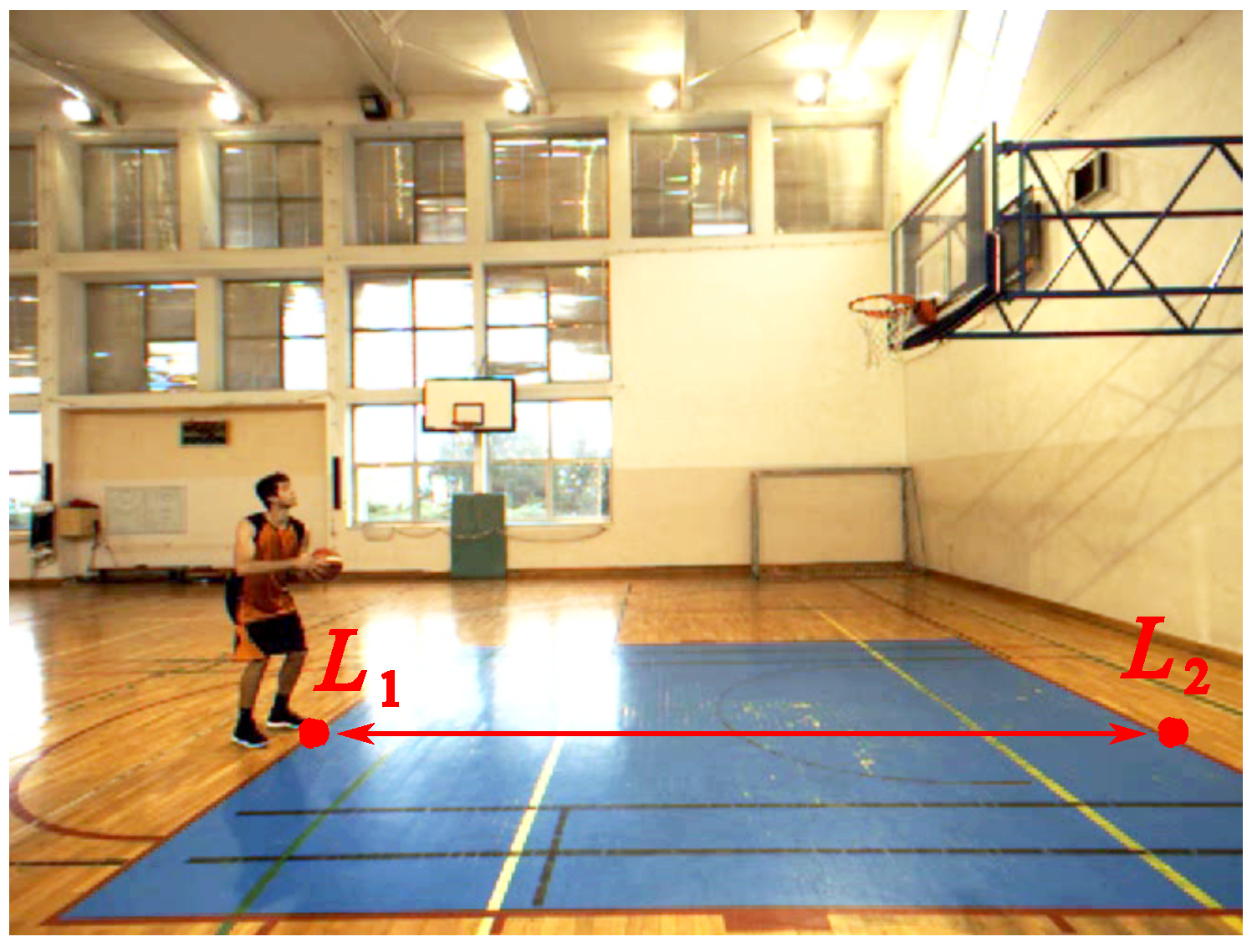
2.2. Camera Calibration

In order to obtain distance parameters from the image, it is necessary to determine the transition from the two-dimensional image space to the three-dimensional space, which allows for the determination of the distance between the objects in the image. In order to maximally simplify the system initialization, a simplified calibration procedure was used. This procedure is based on the distance between the characteristic objects (landmarks) on the scene (the basketball court), such as lines, the intersection of lines, basket, etc. It was assumed that the ball moves perpendicular to the camera, the distance of the ball from the camera during the flight to the basket does not change and the distortions of the camera are negligible. The calibration procedure is limited to the selection of two landmarks on the stage, which is at the same distance from the camera as the ball and giving the distance between them in the image in pixels and the real distance in meters. Given the distance between landmarks in the image, the corresponding distance in the real world and the ball position on the image, the distance parameters of the ball may be estimated. In the presented study, the distance between the free throw line ($L_1$ on Figure 1) and the line defining the end of basketball court ($L_2$ on Figure 1) was used.

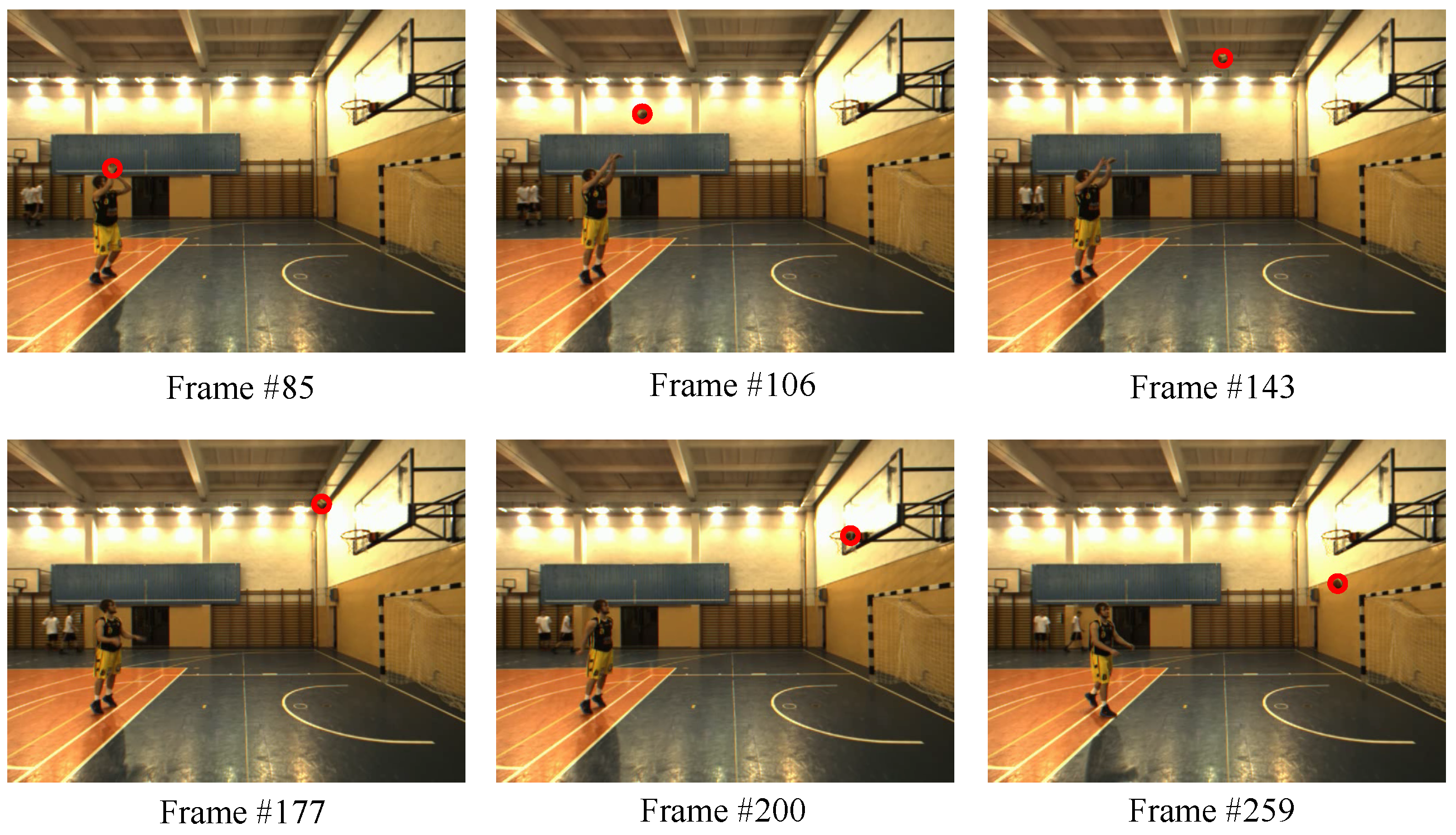
2.3. Basketball Detection

An important part of the system developed to obtain the trajectory of a basketball free throw is the detection of the ball. This ball detection method enables automatic tracking initialization and redetection in case of a tracking failure. To extract the moving objects, the background subtraction algorithm developed by Zivkovic and van der Heijden [39] as well as morphological methods [40] were used. After extraction for each object, two conditions are checked; if both are true, the object is classified as a ball. The first condition concerns the size of the object and is determined by comparing the radius of the enclosing circle of the object with the radius of the ball. The first condition has the form:

$$\left|r_o-r_b\right|<m,$$

(4)

where $r_o$ is the radius of the enclosing circle of the considered object, $r_b$ is the radius of the ball and m is the margin factor, whose value was set at $22\%$ of $r_b$. The parameter $r_b$ is set during calibration; we assume that the change in the size of the ball during flight is negligible. The second condition uses the circularity factor $f_c=\frac{4\pi A}{P^2}$ [41], where A is the area of the object and P is the perimeter of the object. The value of $f_c$ for a perfectly round object is equal to 1. The second condition is described by the formula:

$$T_c<f_c,$$

(5)

where $T_c$ is the circle threshold equal to $0.78$. The values of m and $T_c$ have been determined experimentally. If both conditions are true, it means that the object under consideration is a ball and the tracking process can be started. Additionally, in order to minimize the risk of false detections, all of the objects in the image in front of the free-throw line and simultaneously below the chest of the reference player (player with a height corresponding to the average height of all competitors) are removed.

2.4. Ball Tracking

The proposed method of tracking is a 2D method; its result is the position of the ball in the image in the form of pixel coordinates. In our application, the position of the i-th particle represents the hypothetical position of a ball and the fitness function determines whether a considered part of the image contains the tracked object or not. This function is defined as the ratio of the number of pixels in the extracted objects that are located within the circle defined by the ball position and radius $r_b$ to the number of pixels that are outside the circle.

The block diagram of the ball detection and tracking algorithm is shown in Figure 2. At the beginning, the value of the boolean variable $is\_detected$, which determines if the ball is detected; it is set to FALSE (see block 1 in Figure 2). Next, a new image frame is loaded (block 2) and it is determined whether or not the ball position from the previous frame is known (block 3), if not, the ball detection procedure is started (block 4, see Section 2.3). If the position of the ball in the previous frame is known, then the PSO algorithm is initialized from it (block 6). In the next steps (blocks 7, 8, 9, 10), the algorithm tries to find the current position of the ball. In block 11, the algorithm checks whether the current position of the ball has been determined. If so, the value of the best particle $\mathbf{gbest}$ is assigned to the variable $\mathbf{ball}\_\mathbf{pos}$. Otherwise, the variable $is\_detected$ is set to FALSE. The algorithm ends when there are no more frames available for processing (block 14).

2.5. Parameter Calculations

The parameters of the free throw (see Figure 3) may be calculated using the estimated trajectory. The analysis included ten parameters at three points of the throw. The measured parameters were: velocities in three points ($v_1$, $v_2$, $v_3$), angles of the moving ball (${\alpha }_1$, ${\alpha }_2$, ${\alpha }_3$), height parameters ($h_1$, $h_2$) and a distance parameters ($l_1$, $l_2$). It should be noted that the value of parameter $h_1$ is also closely related to the player’s height, in addition to the player’s technique. A description of the specified parameters is shown in Figure 3. The procedure for calculating the parameters from a 2D ball trajectory is listed below:

• Calculate the 2D coordinates of the ball trajectory using the PSO algorithm.
• Smooth the trajectory using the moving average filter (window = 5),
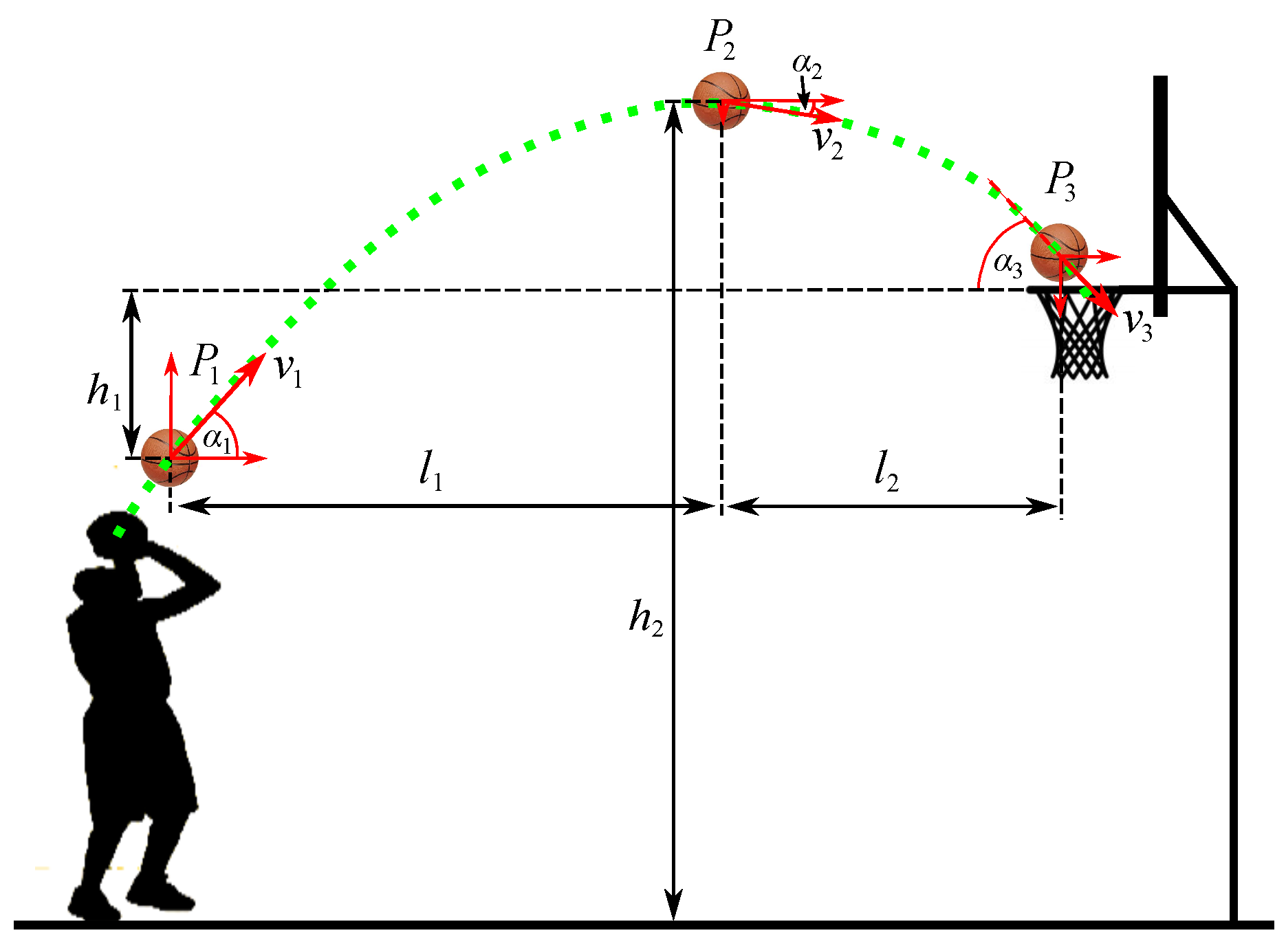
• Determination of auxiliary points ($P_1$—point when the ball leaves player’s hands, $P_2$—the highest point of the ball trajectory and $P_3$—point when the ball makes contact for the first time with the rim line or with the basket board) (Figure 3). Points $P_1$ and $P_3$ determine the range of the analysed trajectory.
• Calculation of altitude and distance parameters on the basis of determined points.
• Determination of auxiliary vectors anchored in the analysed points to determine angular parameters.
• The angular parameters are calculated from the formula:

  $$\alpha ={cos}^{-1}(\frac{\mathbf{v}·\mathbf{h}}{\parallel \mathbf{v}\parallel ·\parallel \mathbf{h}\parallel })·\frac{180}{\pi },$$

  (6)

  where: $\alpha$ is the calculated angle (degrees), $\mathbf{v}$—vertical vector, $\mathbf{h}$—horizontal vector, $\parallel \mathbf{v}\parallel$ is the Euclidean norm of vector $\mathbf{v}$ and $\parallel \mathbf{h}\parallel$ is the Euclidean norm of vector $\mathbf{h}$.
• Conduct a statistical analysis including basic statistical measures, a test of the significance of differences between hit and missed throws, and an analysis of the relationship between the ${\alpha }_1$ and $v_1$ parameters.

2.6. Data Collection

The study was conducted on a group of basketball players who played in the Polish Second Division during the 2015/2016 season and the Youth Polish National Team in 2017. The analysed group consisted of 30 males aged 18.8 ± 2.3. The players were described by the following parameters: body height $188.0\pm 8.7$ cm, body mass 80.4 ± 9.2 kg, and BMI 22.7 ± 1.5. Throughout the research, the sequence of a free throw under regulation conditions was captured. In the analysis, 200 throws were used. The sequences were captured by a monocular 100 Hz Basler Ace acA645-100gc camera (Basler AG, Ahrensburg Germany). The camera was placed 4.6 m from the predicted trajectory of the ball and perpendicular to it. It should be noted that the ideal perpendicular positioning is very difficult to implement under experimental conditions.

3. Results

3.1. Algorithm Evaluation

The system developed for ball tracking was evaluated in 20 video sequences of the basketball free throw. The quality of tracking was determined by analyses carried out through qualitative visual evaluations as well as quantitatively through the use of manually obtained ground truth data. In Figure 4, Figure 5 and Figure 6 the ball tracking results for selected players are presented. In Figure 4 and Figure 5, the ball went into the basket. However, Figure 6 shows a missed shot. It may be observed that the proposed method for tracking the ball has very high levels of accuracy. However, in some situations, tracking errors may occur due to imperfections in the computer vision methods for extracting objects in the scene. For example, in sequence s1 (see Figure 4), the ball was detected later than in the case of other sequences, which resulted in the tracking starting with a delay (see Figure 4, frame #130). Another example may be seen in frame #148 in Figure 4 where the tracking inaccuracies caused by changes in the lighting level on stage may be observed. This change in lighting was caused by the light source being obscured by the ball.

Table 1. Errors for compared methods.

Method			PF					PSO
Particles	50	100	200	300	500	5	10	20	30	50
Iterations	—	—	—	—	—	10	10	10	10	10
RMSE [pixels]	9.89	8.06	8.20	8.80	10.71	10.94	7.22	5.91	5.93	5.82
Tracking failure [number of incidents]	4	1	8	13	13	0	0	0	0	0

presents the Root Mean Square Error (RMSE) for results obtained by PSO and a particle filter (PF) algorithm, which is commonly used for object tracking [21,23,28,29]. The RMSE error for one sequences has the form:

$$RMS{E}_N=\frac{1}{F}\sum _{i=1}^F\sqrt[]{{(x_i-x_i^{GT})}^2+{(y_i-y_i^{GT})}^2},$$

(7)

$$RMSE=\frac{1}{N}\sum _{j=1}^{N}RMS{E}_j,$$

(8)

where: N—is the total number of sequences, F—is the total number of frames, $x_i,y_i$—are the estimated coordinates of the ball, $x_i^{GT},y_i^{GT}$—the manual settings (ground truth) coordinates of the ball.

The ground truth data were obtained by manually pointing out the positions of the ball on the image sequences. For each algorithm, errors were determined for the 5 configurations selected so that for both algorithms the number of calls of the objective function was the same. For most configurations, the PSO algorithm produced much better results, with the exception of the configuration with the smallest number of particles. In addition,

Table 2. Estimated parameters of the free throw trajectory.

Param.	Throws	Body Height of Athletes								All Athletes
		171–180 cm		181–190 cm		191–200 cm		201–210 cm
		$\overline{x}$	$sd$	$\overline{x}$	$sd$	$\overline{x}$	$sd$	$\overline{x}$	$sd$	$\overline{x}$	$sd$	d	p
$h_1$	hit	695	214	678	219	463	237	345	141	542	251
	missed	946	156	732	271	694	292	491	138	723	277	−181.6	0.0001
$h_2$	hit	3861	147	3902	74	3939	186	3915	121	3909	139
	missed	3909	100	3903	120	3926	243	3824	117	3906	184	3.0	0.9004
$l_1$	hit	2307	193	2187	132	2224	133	2093	135	2198	159
	missed	2311	133	2205	165	2139	174	2137	135	2185	170	13.3	0.6061
$l_2$	hit	1614	121	1629	152	1650	215	1696	143	1648	168
	missed	1555	62	1552	144	1553	149	1518	82	1549	129	98	0.0001
${\alpha }_1$	hit	48.8	7.3	55.8	13.7	46.9	9.1	47.4	9.9	50.0	11.2
	missed	50.7	4.6	51.5	13.1	47.2	9.8	46.2	11.2	48.9	10.3	1.2	0.5070
${\alpha }_2$	hit	10.7	2.0	11.0	2.2	11.9	3.7	10.7	2.0	11.2	2.7
	missed	8.8	2.6	10.6	2.3	10.2	2.6	12.1	1.6	10.3	2.5	0.9	0.0336
${\alpha }_3$	hit	45.9	11.2	45.4	8.9	44.5	9.8	44.6	7.1	45.1	9.2
	missed	40.3	5.2	40.6	8.0	38.3	8.6	41.1	12.0	39.5	8.3	−5.5	0.0001
$v_1$	hit	5.5	0.4	5.6	0.8	5.5	0.6	5.3	0.4	5.5	0.6
	missed	5.6	0.2	5.4	0.6	5.7	1.1	5.4	0.2	5.6	0.8	−0.1	0.5171
$v_2$	hit	3.9	0.3	3.9	0.2	4.0	0.3	4.0	0.2	4.0	0.3
	missed	3.9	0.2	3.9	0.3	4.0	0.5	4.1	0.2	4.0	0.4	0.0	-
$v_3$	hit	4.4	1.0	4.6	0.8	4.7	0.7	4.7	0.8	4.6	0.8
	missed	4.6	0.2	4.7	0.5	4.6	0.6	4.3	0.7	4.6	0.5	0.0	-

${}^{\star }$$\overline{x}$—mean,$sd$—standard deviation, d—difference between mean values of missed and hit throws, p—test probability.

contains a number of incidents in which the tracking failed, and redetection was necessary. The best result (RMSE = 5.82 pixels) was obtained for the configuration of 50 particles and 10 iterations of the PSO algorithm.

Figure 7 presents the determined trajectory of the ball in selected sequences. The trajectories were filtered using the moving average filter (window = 5). In the initial phase of tracking, the errors caused by the change in lighting conditions, mentioned earlier, may be observed (see Figure 7, sequence s1) However, it should be noted that these errors can be eliminated by carrying out additional analyses of the ball trajectory.

3.2. Using in Practice

Table 2 shows the basic statistics of the analysed parameters ($\overline{x}$—mean, $sd$—standard deviation, d—difference between the mean values of the missed and hit throws). The table presents data for all athletes grouped by body height. The parameters were calculated from 200 sequences including 155 hit and 45 missed throws. Additionally, to specify the statistical significance of the difference between hit and missed throws the t-Student’s test was used (p).

In the case of the parameter $h_1$, measured from the lowest point of the altitude of the ball relative to the basket height, it may be observed that players who throw the ball into the basket reached the lower value of this parameter of 542 mm. The differences between hit and missed throws for this parameter had a statistical significance ($p<0.001$). This parameter reached the highest value among the shortest competitors (body height 171–180 cm; 695 cm for hit and 946 for missed throws). An analysis of the data showed that the maximum altitude of the ball for all participants ($h_2$) in hit and missed throws were at the same level (approximately 3900 mm). In addition, in the body height groups, there were no significant differences in $h_2$ between hit and missed throws. The distance analysis of the first part of the ball trajectory $l_1$ (measured from $P_1$ to $P_2$—see Figure 3), showed that this parameter was higher for hit throws (2198 mm), but the difference was relatively small ($13.3$ mm). Considering the length $l_2$ (measured from $P_2$ to $P_3$), it may be seen that the hit throws had a longer distance (1648 mm) than the missed throws (1549 m). From analysing the values of $l_2$ for individual height groups, it is noteworthy that, in each case, the value is higher for hit throws. Differences in the $l_2$ parameters are statistically significant ($p<0.001$). The values of the initial angle ${\alpha }_1$ for most players who throw the ball into the basket reaches ${50.0}^{\circ }$. Since, according to earlier studies [42,43], the initial angle of the ball should be about ${52}^{\circ }$, it may be assumed that in such a case we are dealing with a correct throw. In missed throws, this parameter was at the level of ${48.9}^{\circ }$. The analysis conducted also showed that the lowest ${\alpha }_1$ in hit throws occurred for athletes with a body height in the range of 191–200 cm, while the largest angle (${55.8}^{\circ }$) during the throw was obtained by athletes belonging to a group of people with a body height of 181–190 cm. In the case of missed throws, this parameter was placed at the lowest level (${46.2}^{\circ }$) among the tallest athletes. Another analysed parameter is the angle ${\alpha }_2$ (the angle of ball trajectory at the highest point of the trajectory). The angle ${\alpha }_2$ measured during hit throws assumes similar values for each research group with a slight advantage among athletes whose body height is between 191–200 cm. Analysing ${\alpha }_2$ for a missed throw shows that the situation is different. In the group of the shortest athletes, this angle assumes the lowest value at the level of ${8.8}^{\circ }$, and, among the tallest athletes, it reaches the highest value (${12.1}^{\circ }$). For the whole group parameter, ${\alpha }_2$ was slightly higher for hit throws (${\alpha }_2={11.2}^{\circ }$, $p<0.05$). In the case of the angle ${\alpha }_3$, the values of this parameter are larger in the hit throws than in the missed throws ($p<0.001$). However, we should pay attention to players with a body height of 191–200 cm. This group produced the lowest ${\alpha }_3$ values during hits (${44.5}^{\circ }$) and missed (${38.3}^{\circ }$) throws. The last considered parameters are the throw velocities. According to Hamilton and Reinschmidt [8], the optimum speed $v_1$, which is achieved when the ball is thrown, is approximately $7.3$ m/s. By analysing $v_1$, without dividing the height of bodies, for hit and missed throws, it is shown that the velocity assumes similar values ($5.5$ for hit and $5.6$ m/s for missed throws). The lowest velocity $v_1$ in hit throws are produced by the tallest athletes ($5.3$ m/s). In the case of missed throws, the highest value ($5.7$ m/s) of the ball occurs during the throws by almost the tallest athletes (191–200 cm). The conducted analysis also indicated that, regardless of the height of the athlete’s body, for parameters $v_2$ and $v_3$, there were no significant differences in the values of these variables.

According to Ref. [44], we also present the relationship between ${\alpha }_1$ and $v_1$ for all competitors and for individual body height groups as shown in Figure 8. The blue dotted lines present the typical values for the analysed groups. For example, players with a body height of 181 cm to 190 cm should make a throw at $5.6$ m/s and at an angle of about ${56}^{\circ }$. The size of the ellipse surrounding the points represents the dispersion of the results (blue for hit throws, red for missed throws). On the basis of Figure 8, it may be observed that, for all participants, the dispersion of missed throws is significantly larger than the dispersion of hit throws. By analysing the studied dependencies in individual groups, it may be concluded that, among smaller players (171–180 cm and 181–190 cm), missed throws are characterized by a greater dispersion in terms of the parameters $v_1$ and ${\alpha }_1$. Among the tallest players, hit throws are characterized by a higher dispersion value.

4. Conclusions

The paper presents a system for ball detection, tracking and trajectory analysis during a basketball free throw. The experimental results were based on 200 sequences of 30 basketball players. The values of 10 parameters were measured. The results showed the differences between the parameters in missed and correct throws. The analysis showed that significant differences between missed and hit free throws were observed for parameters $h_1$, $l_2$, ${\alpha }_2$ and ${\alpha }_3$. Additionally, an analysis of the relationship between body height and the parameters of the trajectory was calculated.

The proposed method of analysing ball trajectory in free throws may be used in practice by coaches in the training process as a tool to improve the execution of free throws. Coaches using this system will be able to monitor the trajectory of the ball and the parameters of the free throw, which will help to improve the correct motor habit. He can also eliminate some of the technical mistakes of players performing a free throw. On the basis of ${\alpha }_1$ and $v_1$, among other factors, the coach could adjust the player’s body posture (i.e., upper limb positions). They could also pay attention to the initial velocity of the ball—the player may make a throw with more or less strength, which will change the speed of the ball. A basketball coach was consulted concerning the whole idea of the system.

Future work will focus on improving the proposed system and developing an expert system that would allow for the automatic evaluation of performed free throws.

References

1. Yang, X. Research on free throw shooting skills in basketball games. BioTechnol. Indian J. 2014, 10, 11800–11805. [Google Scholar]
2. Gómez, M.Á.; Lorenzo, A.; Jiménez, S.; Navarro, R.M.; Sampaio, J. Examining choking in basketball: Effects of game outcome and situational variables during last 5 minutes and overtimes. Percept. Mot. Skills 2015, 120, 111–124. [Google Scholar] [CrossRef] [PubMed]
3. Gablonsky, J.M.; Lang, A.S. Modeling basketball free throws. SIAM Rev. 2005, 47, 775–798. [Google Scholar] [CrossRef]
4. Liu, Y.; Huang, C.; Liu, X. A New method to classify shots in basketball video. In Proceedings of the Second International Symposium on Networking and Network Security (ISNNS ’10), Minneapolis, MN, USA, 20–22 August 2010; pp. 153–156. [Google Scholar]
5. Perše, M.; Kristan, M.; Kovačič, S.; Vučkovič, G.; Perš, J. A trajectory-based analysis of coordinated team activity in a basketball game. Comput. Vis. Image Underst. 2009, 113, 612–621. [Google Scholar] [CrossRef]
6. Ammar, A.; Chtourou, H.; Abdelkarim, O.; Parish, A.; Hoekelmann, A. Free throw shot in basketball: Kinematic analysis of scored and missed shots during the learning process. Sport Sci. Health 2016, 12, 27–33. [Google Scholar] [CrossRef]
7. Englert, C.; Bertrams, A.; Furley, P.; Oudejans, R.R. Is ego depletion associated with increased distractibility? Results from a basketball free throw task. Psychol. Sport Exerc. 2015, 18, 26–31. [Google Scholar] [CrossRef]
8. Hamilton, G.R.; Reinschmidt, C. Optimal trajectory for the basketball free throw. J. Sports Sci. 1997, 15, 491–504. [Google Scholar] [CrossRef] [PubMed]
9. Button, C.; Macleod, M.; Sanders, R.; Coleman, S. Examining movement variability in the basketball free-throw action at different skill levels. Res. Q. Exerc. Sport 2003, 74, 257–269. [Google Scholar] [CrossRef] [PubMed]
10. Murphy, L. Modeling baskestball free throws. In Proceedings of the 17th Annual Statewide Undergraduate Research Conference, Amherst, MA, USA, 22 April 2012. [Google Scholar]
11. Tran, C.M.; Silverberg, L.M. Optimal release conditions for the free throw in men’s basketball. J. Sports Sci. 2008, 26, 1147–1155. [Google Scholar] [CrossRef] [PubMed]
12. Xu, P.; Xie, L.; Chang, S.F.; Divakaran, A.; Vetro, A.; Sun, H. Algorithms and system for segmentation and structure analysis in soccer video. In Proceedings of the International Conference on Multimedia and Expo 2001 (ICME 2001), Tokyo, Japan, 22–25 August 2001; pp. 928–931. [Google Scholar] [CrossRef]
13. Rahma, A.M.S.; Rahma, M.A.; Rahma, M.A. Automated analysis for basketball free throw. In Proceedings of the Seventh International Conference on Intelligent Computing and Information Systems, Penang, Malaysia, 12–14 December 2015; pp. 447–453. [Google Scholar]
14. Panagiotakis, C.; Grinias, I.; Tziritas, G. Automatic human motion analysis and action recognition in athletics videos. In Proceedings of the 14th European Signal Processing Conference, Florence, Italy, 4–8 September 2006. [Google Scholar]
15. Lenik, P.; Krzeszowski, T.; Przednowek, K.; Lenik, J. The analysis of basketball free throw trajectory using PSO algorithm. In Proceedings of the 3rd International Congress on Sport Sciences Research and Technology Support, Lisbon, Portugal, 15–17 November 2015; pp. 250–256. [Google Scholar]
16. Ramasso, E.; Panagiotakis, C.; Rombaut, M.; Pellerin, D.; Tziritas, G. Human shape-motion analysis in athletics videos for coarse to fine action/activity recognition using transferable belief model. Electron. Lett. Comput. Vis. Image Anal. 2009, 7, 32–50. [Google Scholar] [CrossRef]
17. Elliott, N.; Choppin, S.; Goodwill, S.R.; Allen, T. Markerless tracking of tennis racket motion using a camera. Procedia Eng. 2014, 72, 344–349. [Google Scholar] [CrossRef]
18. Barros, R.M.; Menezes, R.P.; Russomanno, T.G.; Misuta, M.S.; Brandão, B.C.; Figueroa, P.J.; Leite, N.J.; Goldenstein, S.K. Measuring handball players trajectories using an automatically trained boosting algorithm. Comput. Methods Biomech. Biomed. Eng. 2010, 14, 53–63. [Google Scholar] [CrossRef] [PubMed]
19. Sheets, A.L.; Abrams, G.D.; Corazza, S.; Safran, M.R.; Andriacchi, T.P. Kinematics differences between the flat, kick, and slice serves measured using a markerless motion mapture method. Ann. Biomed. Eng. 2011, 39, 3011–3020. [Google Scholar] [CrossRef] [PubMed]
20. Chen, H.T.; Chou, C.L.; Fu, T.S.; Lee, S.Y.; Lin, B.S.P. Recognizing tactic patterns in broadcast basketball video using player trajectory. J. Vis. Commun. Image Represent. 2012, 23, 932–947. [Google Scholar] [CrossRef]
21. Gomez, G.; López, P.H.; Link, D.; Eskofier, B. Tracking of ball and players in beach volleyball videos. PLoS ONE 2014, 9, e111730. [Google Scholar] [CrossRef] [PubMed]
22. Tawab, A.M.A.; Abdelhalim, M.; Habib, S.D. Efficient multi-feature PSO for fast gray level object-tracking. Appl. Soft Comput. 2014, 14, 317–337. [Google Scholar] [CrossRef]
23. Nummiaro, K.; Koller-Meier, E.; Gool, L.V. An adaptive color-based particle filter. Image Vis. Comput. 2003, 21, 99–110. [Google Scholar] [CrossRef] [Green Version]
24. Chen, H.T.; Tsai, W.J.; Lee, S.Y.; Yu, J.Y. Ball tracking and 3D trajectory approximation with applications to tactics analysis from single-camera volleyball sequences. Multimed. Tools Appl. 2012, 60, 641–667. [Google Scholar] [CrossRef]
25. Kurano, J.; Hayashi, M.; Yamamoto, T.; Kataoka, H.; Tanabiki, M.; Furuyama, J.; Aoki, Y. Ball trajectory extraction in team sports videos by focusing on ball holder candidates for a play search and 3D virtual display system. J. Signal Process. 2015, 19, 147–150. [Google Scholar] [CrossRef]
26. Hou, Y.; Cheng, X.; Ikenaga, T. Real-time 3D ball tracking with CPU-GPU acceleration using particle filter with multi-command queues and stepped parallelism iteration. In Proceedings of the 2nd International Conference on Multimedia and Image Processing (ICMIP), Wuhan, China, 17–19 March 2017; pp. 235–239. [Google Scholar]
27. Wang, X.; Ablavsky, V.; Shitrit, H.B.; Fua, P. Take your eyes off the ball: Improving ball-tracking by focusing on team play. Comput. Vis. Image Underst. 2014, 119, 102–115. [Google Scholar] [CrossRef] [Green Version]
28. Wang, Y.; Cheng, X.; Ikoma, N.; Honda, M.; Ikenaga, T. Motion prejudgment dependent mixture system noise in system model for tennis ball 3D position tracking by particle filter. In Proceedings of the Joint 8th International Conference on Soft Computing and Intelligent Systems (SCIS) and 17th International Symposium on Advanced Intelligent Systems (ISIS), Sapporo, Japan, 25–28 August 2016; pp. 124–129. [Google Scholar]
29. Cheng, X.; Zhuang, X.; Wang, Y.; Honda, M.; Ikenaga, T. Particle filter with ball size adaptive tracking window and ball feature likelihood model for ball’s 3D position tracking in volleyball analysis. In Advances in Multimedia Information Processing—PCM 2015; Ho, Y.S., Sang, J., Ro, Y.M., Kim, J., Wu, F., Eds.; Springer International Publishing: Cham, The Netherlands, 2015; pp. 203–211. [Google Scholar]
30. Alexander, M.J.; Hayward-Ellis, J. The effectiveness of the shotloc training tool on basketball free throw performance and technique. Int. J. Kinesiol. Sports Sci. 2016, 4, 43–54. [Google Scholar]
31. Marty, A.; McGhee, R.; Edwards, T. Trajectory Detection and Feedback System. U.S. Patent 11/508,004, 16 January 2007. [Google Scholar]
32. Kennedy, J.; Eberhart, R. Particle swarm optimization. In Proceedings of the International Conference on Neural Networks, Perth, Western Australia, 27 November–1 December 1995; IEEE Press: Piscataway, NJ, USA, 1995; Volume 4, pp. 1942–1948. [Google Scholar]
33. Eberhart, R.C.; Shi, Y. Comparing inertia weights and constriction factors in particle swarm optimization. In Proceedings of the Congress on Evolutionary Computation, La Jolla, CA, USA, 16–19 July 2000; Volume 1, pp. 84–88. [Google Scholar] [CrossRef]
34. Kwolek, B. Object tracking via multi-region covariance and particle swarm optimization. In Proceedings of the 11th IEEE International Conference on Advanced Video and Signal Based Surveillance (AVSS), Washington, DC, USA, 2–4 September 2009; pp. 418–423. [Google Scholar] [CrossRef]
35. Mussi, L.; Ivekovic, S.; Cagnoni, S. Markerless articulated human body tracking from multi-view video with GPU-PSO. In Evolvable Systems: From Biology to Hardware; Tempesti, G., Tyrrell, A.M., Miller, J.F., Eds.; Springer: Berlin/Heidelberg, Germany, 2010; pp. 97–108. [Google Scholar]
36. John, V.; Trucco, E.; Ivekovic, S. Markerless human articulated tracking using hierarchical particle swarm optimisation. Image Vis. Comput. 2010, 28, 1530–1547. [Google Scholar] [CrossRef]
37. Kwolek, B.; Krzeszowski, T.; Gagalowicz, A.; Wojciechowski, K.; Josinski, H. Real-time multi-view human motion tracking using particle swarm optimization with resampling. In Articulated Motion and Deformable Objects; Lecture Notes in Computer Science; Perales, F., Fisher, R., Moeslund, T., Eds.; Springer: Berlin/Heidelberg, Germany, 2012; Volume 7378, pp. 92–101. [Google Scholar] [CrossRef]
38. Michel, D.; Panagiotakis, C.; Argyros, A.A. Tracking the articulated motion of the human body with two RGBD cameras. Mach. Vis. Appl. 2015, 26, 41–54. [Google Scholar] [CrossRef]
39. Zivkovic, Z.; van der Heijden, F. Efficient adaptive density estimation per image pixel for the task of background subtraction. Pattern Recogn. Lett. 2006, 27, 773–780. [Google Scholar] [CrossRef]
40. Haralick, R.M.; Sternberg, S.R.; Zhuang, X. Image analysis using mathematical morphology. IEEE Trans. Pattern Anal. Mach. Intell. 1987, 9, 532–550. [Google Scholar] [CrossRef] [PubMed]
41. Ritter, N.; Cooper, J. New resolution independent measures of circularity. J. Math. Imaging Vis. 2009, 35, 117–127. [Google Scholar] [CrossRef]
42. Hudson, J.L. A biomechanical analysis by skill level of free throw shooting in basketball. Biomech. Sports 1982, 1, 95–102. [Google Scholar]
43. Chen, H.T.; Tien, M.C.; Chen, Y.W.; Tsai, W.J.; Lee, S.Y. Physics-based ball tracking and 3D trajectory reconstruction with applications to shooting location estimation in basketball video. J. Vis. Commun. Image Represent. 2009, 20, 204–216. [Google Scholar] [CrossRef]
44. Inaba, Y.; Hakamada, N.; Murata, M. Influence of selection of release angle and speed on success rates of jump shots in basketball. In Proceedings of the 5th International Congress on Sport Sciences Research and Technology Support, Funchal, Madeira, Portugal, 30–31 October 2017; pp. 48–55. [Google Scholar] [CrossRef]
Figure 1. Block diagram of the ball detection and tracking algorithm.
Applsci 08 02090 g001
Figure 2. Block diagram of the ball detection and tracking algorithm.
Applsci 08 02090 g002
Figure 3. Analysed parameters of a basket throw; h 1 [m]—height between ball and basket, h 2 [m]—height of ball parabola, l 1 [m]—distance between 1st and 2nd point, l 2 [m]—distance between 2nd and 3rd point, v 1 [m/s]—velocity of ball in 1st point, v 2 [m/s]—velocity of ball in 2nd point, v 3 [m/s]—velocity of ball in 3rd point, α 1 [ ] —angle of ball in 1st point, α 2 [ ] —angle of ball in 2nd point, α 3 [ ] —angle of ball in 3rd point.
Applsci 08 02090 g003
Figure 4. Ball tracking in selected frames of sequence s1.
Applsci 08 02090 g004
Figure 5. Ball tracking in selected frames of sequence s11.
Applsci 08 02090 g005
Figure 6. Ball tracking in selected frames of sequence s148.
Applsci 08 02090 g006
Figure 7. Ball trajectory for selected sequences.
Applsci 08 02090 g007
Figure 8. Relationships between α 1 and v 1 parameters.
Applsci 08 02090 g008