Abstract
Continuous power supply for unmanned and automatic observation systems without suitable energy-storage capabilities in the polar regions is an urgent problem and challenge. However, few power-supply systems can stably operate over the long term in extreme environments, despite excellent performance under normal environments. In this study, a standalone hybrid wind–solar system is proposed, based on operation analysis of the observing system in the Arctic Ocean, the polar environments, and renewable-energy distribution in the polar regions. Energy-storage technology suitable for cold regions is introduced to support the standalone hybrid wind–solar system. Mathematical models of the power system at low temperature are also proposed. The low-temperature performance and characteristics of lead–acid battery are comprehensively elucidated, and a dedicated charging strategy is developed. A hybrid wind–solar charging circuit is developed using a solar charging circuit, a wind turbine charging circuit, a driver circuit, a detection circuit, an analog-to-digital converter (ADC) circuit, and an auxiliary circuit. The low temperature stability of charging circuit is test from −50 °C to 30 °C. Temperature correction algorithm is designed to improve the efficiency of the power supply system. The power generation energy of the power system was simulated based on the monthly average renewable energy data of Zhongshan Station. A case study was applied to examine the technical feasibility of the power system in Antarctica. The five-month application results indicate that the power system based on renewable energy can maintain stable performance and provide sufficient power for the observing system in low ambient temperatures. Therefore, this power system is an ideal solution to achieve an environmentally friendly and reliable energy supply in the polar regions.
1. Introduction
The extent and thickness of Arctic sea ice have dramatically declined in recent decades, which is considered one of the most impactful changes to Earth’s surface [1,2]. The conditions of Arctic sea ice cover can be effectively measured using various means. The mass balance of sea ice has been recorded with noncontact instruments, such as upward-looking sonar and electromagnetic induction devices (EM-31) on a helicopter or ship [3,4,5], and contact instruments, such as ice-based buoys. Various ice-based buoys have been deployed for field observation of sea ice in the Arctic Ocean and Antarctica. Ice mass-balance buoys (IMBs) [6] and sea-ice mass-balance buoys (SIMBs) [7] enable the automatic observation of sea-ice thickness, snow depth, and sea-ice temperature profiles. For different depths of sea ice, the spectral intensity of solar radiation can be effectively measured using a fiber optic spectrometry system [8], and the design of the corresponding driver circuit was reported. All ice-based buoys are designed to achieve automatic and continuous observation of sea ice during annual cycles. However, very few buoys have achieved observation of sea ice for more than one year in the polar regions. The possible reasons for premature failure of buoys include: (1) decay of sea ice, (2) running out of power, (3) wild-animal damage, and (4) failure of the instrument itself. The robustness of observation equipment can be improved to protect against destruction by wildlife. In addition, the stability of the instrument has been greatly improved in recent years through continuous field tests and laboratory tests. In the Chinese National Arctic Research Expedition (CHINARE) from 2003 to 2017, the impact of premature sea-ice melting was overcome by locating the instruments in areas with suitable ice thickness and floe location [9,10]. The power-supply problem is the most potential challenge for observation equipment used in the polar region to work for a long time.
Due to the special geographical location of the Arctic Ocean and Antarctica, the design of the power system used in the polar regions has special demands. Burning fossil fuels in the polar regions causes environmental pollution and is therefore restricted. Thus, new demands for clean and sustainable energy such as wind, solar, hydro, and ocean energy have been created. In the polar regions, renewable energy systems (RESs) based on wind and solar energy are considered a clean, inexhaustible, and environmentally friendly method. Solar- and wind-energy resources usually have fluctuations; thus, a hybrid wind–solar system is developed to solve the problem of energy fluctuations in the polar regions. Some work has presented research on hybrid wind–solar systems. For instance, based on the long-term recorded data of wind speed and irradiance, a calculation methodology of a PV array for a standalone hybrid wind/PV system was developed to improve the ability to find the optimum size of the PV array [11]. A report by Reference [12] indicates methodologies to model components and designs of hybrid renewable energy systems, and evaluates them. A case study of isolated site Potou in the northern coast of Senegal also described methodology based on a multiobjective genetic algorithm to realize the optimization of a hybrid solar–wind–battery system, and indicates the influence of load profiles on optimal configuration [13]. More accurate mathematical models for characterizing the PV module, wind generator, and battery were used to achieve the configurations of various types and capacities of system devices by changing the type and size of the devices’ systems [14]. A hybrid system was proposed and applied in many cities in Iraq, which can be considered a renewable resource of power generation. The simulation calculation of this system was done by software based on local meteorological data and the sizes of PV and wind turbines. The results illustrate that it is useful to utilize the solar and wind energy to generate power in harsh environments [15].
Wind and solar energy are unpredictable and weather-dependent in the polar regions. An energy-storage system (ESS) is necessary as a reliable back-up to the observing system in order to store excess energy and then release the power to guarantee periods when a net load occurs. Some integrated wind–PV–battery hybrid systems and power-management strategies were proposed to offer a lower cost and higher efficiency [16]. Isolated power systems built by hybridizing renewable-power sources (wind and solar) in Indian used a battery as appropriate energy storage [17]. Studies [18,19] have developed an energy-management strategy and new photovoltaic solar structure for a renewable-energy system for rural communities to meet load demands. The observation equipment used in cold regions often uses batteries as power storage. However, batteries are sensitive to low temperatures, which can decrease their capacity. Therefore, a hybrid wind- and solar-energy system is also temperature-dependent.
In this study, a new observing system was designed to observe multiple parameters of polar environments based on analysis of the previous deployment of the observing system in the Arctic Ocean. Mathematical models of the PV array, wind turbine, and low-temperature characteristics of a PV panel are proposed. A lead–acid battery was selected for the standalone hybrid wind–solar system. Since battery capacity varies at different ambient temperatures, battery capacities must be calibrated based on charging and discharging experiments at low temperatures. Charging strategy for a battery in polar environments was also designed. A hybrid wind–solar charging circuit was developed to provide a reliable power supply to the observing system by adapting to the low ambient temperature in the Arctic Ocean and Antarctica. This hybrid wind–solar charging circuit is composed of a solar charging circuit, a wind-turbine charging circuit, a detection circuit, an analog-to-digital converter ADC circuit, and an auxiliary circuit [20]. We have comprehensively evaluated the temperature dependence of the circuit with laboratory experiments from −50 °C to 30 °C. The monthly average energy production from the PV panel and the wind turbine were simulated using monthly average meteorological data. A case study of the operational results of the power system during field observations in Zhongshan Station, East Antarctica was examined to evaluate the technical feasibility and stability of the hybrid wind–solar system.
In these contexts, this paper focused on exploring a standalone hybrid wind–solar system for automatic observation systems designed to be used in the polar regions. Section 2 describes the considerations of the observing system and the power system. Section 3 gives the results of the experiment on the low-temperature characteristics of batteries. The design of the hybrid wind–solar charging circuit is given in Section 4, and the performance of the circuit is evaluated in Section 5. The results of the simulation of monthly average energy production from the PV panel and the wind turbine, and a case study of a field experiment in Zhongshan Station, East Antarctica are presented in Section 6. The conclusions are presented in final section.
2. Observing-System and Power-System Considerations
2.1. Deployment of Observing System in the Arctic Ocean
As shown in Figure 1a, an observing system was deployed on Arctic sea ice on 9 August 2016 during the 2016 Chinese National Arctic Research Expedition. This observing system was designed by the Polar Research Institute of China (PRIC) and Taiyuan University of Technology (TYUT), which included an acoustic sounder (SR50A, Campbell, Camden, NJ, USA) and an underwater sonar (PSA-916, Teledyne Benthos, North Falmouth, MA, USA) to measure snow depth and ice thickness, a 4.5 m long thermistor string, a temperature sensor (HMP155A, Vaisala, Vantaa, Finland), a battery unit, a data logger developed by TYUT, and an Iridium system. The power of this system was only dependent on the battery unit (13.5 V, 75 Ah). Blizzard weather occurred three days after the observation system was deployed (Figure 1b); these storms occur frequently in the Arctic Ocean. In Figure 1b, we can see that the situation in which the observing system was deployed had dramatically changed, increasing the possibility of equipment damage.
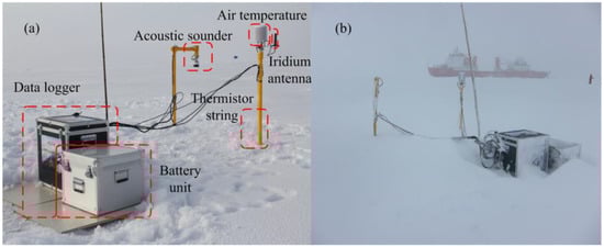
Figure 1.
(a) Observing system deployed in the Arctic Ocean during the 2016 Chinese National Arctic Research Expedition. (b) Scene after three days of observing-system deployment.
The observing system observed the entire ice season for approximately 11 months. As shown in Figure 2, air temperature and power voltage from October 2016 to July 2017 are presented, which covered the period of the polar night. The sampling interval of air temperature and voltage was one hour.
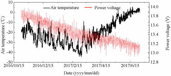
Figure 2.
Air temperature and power voltage of the observing system from October 2016 to July 2017.
The air temperature monitored by the observing system in the entire ice season included one peak (Figure 2). Beginning with the deployment of the observing system, air temperature continued to decrease until 18 February 2017. Subsequently, air temperature continued to increase until 5 July 2017. Power voltage was greatly affected by air temperature, and daily changes were relatively severe and showed an oscillating downward trend. Low temperature was the main influencing factor of the power supply of the observing system. Although power voltage stayed above 13 V, which can ensure the normal operation of the observation system, the continuous decline of power and the violent fluctuation of voltage could bring great potential hazards to the normal operation of the equipment. Thus, designing and developing energy-harvesting systems at low temperatures is vital for long-term observations of the polar regions.
2.2. Environmental Analysis
A power system of the special observation equipment for the polar regions should fully consider the characteristics of the polar natural environment. China’s Zhongshan Station was selected as the one of the deployment locations of the observing system in Antarctica, and its monthly meteorological data (69.37° S, 76.38° E) in Antarctica in recent years are shown in Figure 3, including monthly average wind speed, radiation, day length, and air temperature. The meteorological data in Figure 3 were obtained from NASA’s atmospheric science data center. In Figure 3a, we can see that the distribution of wind speed was approximately parabolic, and monthly average wind speed for the whole year was greater than 7.50 m/s. The maximum monthly average wind speed (9.88 m/s) was in June. The minimum monthly average wind speed (7.50 m/s) was in January. The monthly mean wind speed was consistent with seasonal changes in the southern hemisphere. The average monthly wind speed reached 9.02 m/s. Thus, wind resources around Zhongshan Station were relatively rich to establish power-supply systems for wind-power generation. Figure 3b shows the monthly average radiation near Zhongshan Station. Radiation decreased from 6.05 KWh/m2/day in January to 0.05, 0.00, and 0.01 KWh/m2/day in May, June, and July, respectively. After that, radiation rose from August until December, reaching maximum value (6.69 KWh/m2/day) in one year. The average monthly radiation was 2.49 KWh/m2/day. The results of monthly average day length are shown in Figure 3c. Similar to the results of the radiation shown in Figure 3b, day length decreased from January (24 h) to the minimum value of 0 h in June. Then, day length increased from July until December, reaching the maximum value of 24 h. As can be seen from Figure 1c, Zhongshan Station was in the polar day from December to January of the following year. In June and July, Zhongshan Station was in the polar night, and solar-radiation energy was equal to zero. Average monthly day length was 12.2 h. Figure 3d shows the monthly average air temperature near Zhongshan Station. The maximum monthly mean temperature was −7.13 °C in January. The minimum monthly mean temperature was −27.3 °C in July. Average monthly air temperature was −19.1 °C.
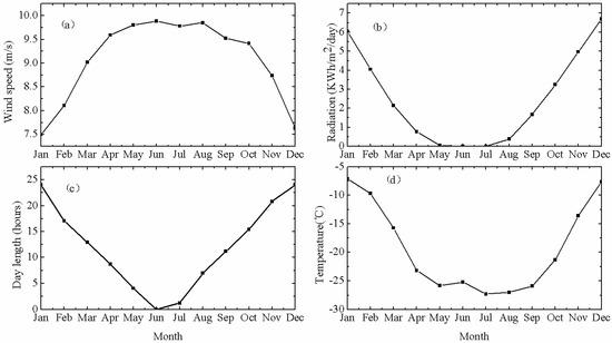
Figure 3.
Monthly meteorological data of Zhongshan Station, Antarctica. (a–d) Monthly wind speed, solar radiation, day length, and air temperature, respectively.
Solar power is the most widely used field power supply in the polar regions, but the polar night limits the time of its application. Although the polar night is only two months, this period has the lowest temperature of the year, which often leads to the obstruction of power-supply systems. When solar energy is minimal in June or July, this happens when wind energy is the strongest, so a hybrid wind–solar power-supply system could be established.
We also planned to deploy our observing system in the Arctic Ocean to observe sea ice parameters. The drift trajectory (Figure 4a) of an Ice Mass-Balance (IMB) buoy and the observed temperature data (Figure 4b) from 10 September 2012 to 16 January 2014 are shown in Figure 4. Figure 4b shows that maximum temperature was 5.93 °C on July 2013. Minimum temperature was −45.06 °C on February 2013. Average temperature was −15.34 °C.
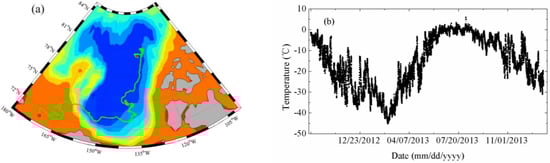
Figure 4.
(a) Drift trajectory (green line) of an Ice Mass-Balance buoy from 10 September 2012 to 16 January 2014 in the Arctic Ocean. (b) Air temperature measured by the buoy.
Based on analysis of meteorological data in the polar regions, the operating temperature range of the power-supply system in this study should be −50–30 °C. The design of the observing system and the power-supply system should consider the effects of low temperatures and other meteorological elements.
2.3. New Observing System and Power System
Based on the analysis of Section 2.1 and Section 2.2, we designed a new observation system and power system, and adjusted the observation parameters of the sensor. The accuracy and temperature range of the sensor were fully considered. Table 1 summarizes the various sensors used in our observing system on the Arctic and Antarctic ice cover. The observing system of ice mass balance consisted of a wind-speed and a direction sensor, a temperature and humidity sensor (HMP155A, Vaisala, Vantaa, Finland), an atmospheric-pressure sensor (CS106/PTB110, Vaisala, Vantaa, Finland), and a 10 m long thermistor string and two spectroradiometers (TriOS, TriOS Optical Sensors, Oldenburg, Germany). The wind-speed and direction sensor was developed by TYUT, designed to overcome the effects of frozen environments by relying on self-heating strings around the sensor. The 10 m long thermistor string was also designed by TYUT and successfully observed the temperature profiles of shallow ice cover.

Table 1.
Sensor information of the observing system.
As shown in Figure 5, the power-supply system of the observing system of the ice mass balance involved in this study is equipped with a power generator that includes the PV array and small wind turbine (SWT), an energy-storage system (a low-temperature battery pack), an end user (load), and a control station (hybrid wind-solar charging circuit). The whole power system is a standalone system. This power-supply system was specifically designed for our small ice mass-balance station. In the design process of the hybrid wind–solar charging circuit, three subcircuits were developed: (1) SWT charging circuit: A three-phase rectifier circuit is required to convert the three-phase alternating current generated by the small wind turbine into a stable direct current. After the rectified and filtered direct current passes through the chopper circuit, it becomes a stable direct current and supplies power to the load or the battery. (2) Solar charging circuit: It is necessary to design a suitable DC chopper circuit and implement the control strategy for the solar charging circuit by adjusting the conversion circuit. (3) Detection circuit and ADC circuits: These subcircuits are mainly used to monitor solar-battery voltage and current, SWT voltage and current, battery voltage, and charging current.
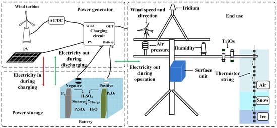
Figure 5.
Schematic of the power-supply system.
Battery capacity generally decreases at lower ambient temperatures. Therefore, the capacity of battery at low-temperature ranges (−50–30 °C) should be completely understood to make the observing system work properly and stably. The performance of the ADC, detection, and auxiliary circuits at low temperatures should be considered, which may affect the charging strategy of the charging circuit.
2.4. Mathematical Modeling of the Power System
2.4.1. PV Array
In this study, polycrystalline PV panels were designed and assembled by TYUT. In the Arctic Ocean and Antarctica, all PV panels were designed to be positioned in a fixed direction parallel to the ground, which can be considered an optimum angle for PV panels installed in the polar regions. The key specifications of the TYUT PV panel are presented in Table 2.
Table 2.
Key specifications of the TYUT PV panel.
The relationship between output of solar power and radiation intensity based on an individual PV cell can be obtained from the Equation (1):
where Esolar is the output of solar power (Wh/day); Pmax is the maximum power at standard test conditions (15 W); T is the ambient temperature (°C); Tstc is the ambient temperature at standard test conditions (25 °C); R is the average radiation intensity (KWh/m2/day); β1 is the soiling losses factor 0.97; β2 is the non-MPPT point coefficient 0.96; β3 is antireverse diode coefficient 0.98.
2.4.2. Wind Turbine
The wind turbine from TYUT was employed in the power system of this study. The key specifications of the TYUT wind turbine are presented in Table 3.
Table 3.
Key specifications of the TYUT wind turbine.
Different wind-turbine types put out different power based on their power-curve characteristics. Through a comprehensive literature review, a model used to describe the performance is proposed as follows [21]:
where Ewind is the output of wind power (Wh/day), which consists of Ea and Eb; vc is the cut-in wind speed (3 m/s); vR is the rated wind speed (10 m/s); vF is the cut-off wind speed (40 m/s); v is the wind speed; PR is the rated electrical power (10 W), which is average energy at the wind speed of 10 m/s for one minute; and t is the time (hours).
2.4.3. Low-Temperature Characteristics of PV Panel
The PV panel is the major power-generation unit of the power system in this study. The environmental characteristics of the installation location of the power-supply system are described in Section 2.1. We do not understand the power-generation characteristics of photovoltaic panels at low temperatures. Therefore, the characteristics of PV panels at low temperatures require a comprehensive study. The key parameters of the PV panel have been described as follows:
where Isc is the short circuit current (A); Voc is the open circuit voltage (V); Imp is the optimum operating current (A); Vmp is the optimum operating voltage (V). Isc, Voc, Imp and Vmp can be found in Table 2. σ1 and σ2 are the are parameters for the convenience of describing the model; isc(R, T) is the short circuit current (A) at radiation intensity R (Wh/m2/day) and ambient temperature T (°C); voc(R, T) is the open circuit voltage (V) at the same conditions as isc(R, T); imp(R, T) and vmp(R, T) are the optimum operating current (A) and voltage (V) at radiation intensity R (Wh/m2/day) and ambient temperature T (°C), respectively; Rr is the reference value of 1000 W/m2; Tr is the reference temperature of 25 °C; a is 0.0025; b is 0.0005; c is 0.00288.
Based on the established PV panel parameter model as shown in Equation (3), the temperature was set 0 °C. Simultaneously, radiation intensities of 1000, 800, 600, and 400 W/m2 were selected for the PV panel. Then, the output characteristics were tested (Figure 6). Figure 6a shows the open circuit voltage and short circuit current of the PV panel. At the same temperature, as radiation intensity decreased, the open circuit voltage and short circuit current of the PV panel would gradually decrease. Figure 6b shows the output power of the PV panel. The output power of the PV panel also increased as the radiation intensity increased. When radiation intensity was kept constant at 1000 W/m2 and ambient temperature was raised from −50 °C to −20 °C, the output characteristics of the PV panel were as shown in Figure 6c,d. Figure 6c shows that the open circuit voltage of the PV panel increased as the temperature decreased, but the short circuit current decreased. Figure 6d shows that the maximum power point of the PV panel increased with decreasing temperature. Although the short circuit current of the PV panel was reduced, the maximum output power point increased in the low-temperature environment.
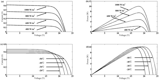
Figure 6.
(a,b) Output characteristics of PV panel under different radiation intensities at the same temperature (0 °C). (c,d) Output characteristics of PV panel under 1000 W/m2 at different temperatures.
3. Experiment on Low-Temperature Battery Characteristics
As shown in Figure 5, a lead–acid battery was used as an energy-storage device for the power-supply system of the observing system. The lead–acid batteries used in our observing system were developed by Taiyuan University of Technology. We used Pb as the negative active material of lead–acid batteries, PbO2 as the positive active material, and diluted H2SO4 as the electrolyte. The chemical reaction principle is shown in Equation (4).
When a lead–acid battery is subjected to a discharge reaction, the Pb on the cathode plate, PbO2 on the anode plate, and the diluted H2SO4 in the surrounding area chemically react, consuming diluted H2SO4 in the electrolyte, and simultaneously forming compounds PbSO4 and H2O. After the discharge behavior, H2SO4 in the electrolyte is gradually consumed, and the longer the discharge time of the battery is, the lower the concentration of H2SO4 in the electrolyte will be.
When the lead–acid battery is charged, H2SO4, Pb, and PbO2 are formed on the cathode and anode plates. Then, the concentration of H2SO4 in the electrolyte gradually recovers. As the charging reaction continues, the H2SO4 concentration slowly returns to its concentration at the beginning of the discharge. At this time, the active substances of the cathode and anode electrodes in the lead–acid battery can be considered to have recovered their activity. When the PbSO4 of the cathode and anode plates is completely reduced to Pb and PbO2, the battery is considered full and the charging process is complete.
3.1. Low-Temperature Calibration Experiment of the Battery Capacity
The activity of the electrolyte of the lead–acid battery is affected by low temperatures, which affect the capacity of the battery. A battery-capacity at low temperatures experiment was designed and implemented.
In the experiment, to calibrate battery capacity, we placed the self-developed lead–acid battery into a GDJS series low-temperature test chamber, which can provide stable environmental temperature. The temperature range for the experiment was from −50 °C to 0 °C. The ideal capacity of the battery is 13.6 V and 75 Ah under a normal temperature environment. We discharged the battery at 7.5 A at different ambient temperatures (−50–0 °C) to determine battery capacity. The voltages of battery were measured by an oscilloscope (MSO70404C, Tektronix, Beaverton, OR, USA), and the discharge cut-off voltage was 10.5 V. The interval for the experimental temperature change was set to 10 °C. At each temperature in the experiment, the low-temperature test chamber maintained the temperature at which battery voltage reached the discharge cut-off voltage. We took the average values of the voltage to minimize statistical error and uncertainty.
The experiment results are shown in Figure 7 and demonstrate that, when a lead–acid battery is discharged with a constant current in a low-temperature environment, the overall trend of the discharge process is similar. As temperature decreased, the discharge time of the battery also decreased at a constant current. This finding indicates that the discharge capacity of the battery was weakening, simultaneously, the amount of discharged electricity decreased. Lead–acid batteries have a capacity of 75.6 (100%), 65 (85.9%), 51.25 (67.8%), 37.5 (49.6%), 28.75 (38%), and 22.5 Ah (29.7%) at 0 °C, −10 °C, −20 °C, −30 °C, −40 °C, −50 °C, respectively. When the temperature was higher than 0 °C, battery capacity remained nearly constant.
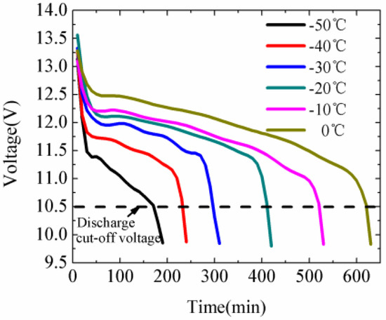
Figure 7.
Discharge curves of the lead–acid battery at low temperatures.
3.2. Low-Temperature Charging Experiment of Lead–Acid Battery
Low ambient temperatures affect the charging capacity of a lead–acid battery. Similar to the experiment to calibrate battery capacity, in the charging experiment, we put the self-developed lead–acid battery into a low–temperature test chamber, and a two-stage charging mode was adopted. In the first stage, we charged the lead–acid battery with a constant current, and at the second stage with constant voltage charging. The temperature range for the experiment was −50–0 °C. The voltage for constant voltage charging was selected to be 14.6 V. The currents of constant current charging were selected as 1, 2, and 3 A, respectively, performed at each temperature. The interval of the experimental temperature change was 10 °C. Each process of charging was repeated, and the voltage–time curves were obtained at the different temperatures. Three experimental sets of curves are shown in Figure 8.
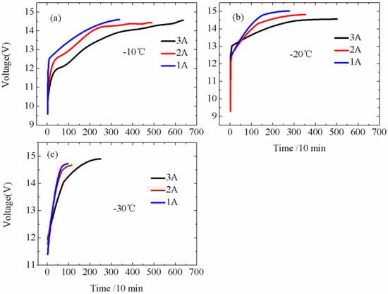
Figure 8.
(a–c) Charging curve for the lead–acid battery at temperatures of −10, −20, and −30 °C under the charging currents of 1, 2, and 3 A, respectively.
As shown in Figure 8, we found that, at the same temperature, the capacity of the battery differed due to different charging currents. The battery-capacity calculation results of the charging experiment are shown in Table 4.
Table 4.
Battery-capacity calculation results of the charging experiment.
The results in Table 4 demonstrate that the battery capacity at −10 °C was 40.0 Ah, 45.4 Ah, and 47.1 Ah with charging currents of 1 A, 2 A, and 3 A, respectively. The battery capacity increased with the charging currents. However, when the experimental temperature was −20 °C, the relationship between the battery capacity and charging current was different from that at −10 °C. The battery capacity at −20 °C was 30.0 Ah, 27.4Ah, and 25 Ah with charging currents of 1 A, 2 A, and 3 A, respectively. Hence, the battery capacity decreased with the increase of the charging currents from 1 A to 3 A. This phenomenon occurred mainly because the drop in ambient temperature to a certain level decreased the activity of the active material on the two-electrode plates of the lead-acid battery decreased, resulting in a slower chemical reaction rate. The battery capacity at −30 °C was 16.7 Ah, 16.5 Ah, and 16.2 Ah with charging currents of 1 A, 2 A, and 3 A, respectively. The battery capacity under different charging currents changed little, because the activity of the active material on the two-electrode plates was further reduced.
3.3. Charging Strategy
Based on the experimental results in Section 3.1 and Section 3.2, the magnitude of the charging current would affect the actual capacity of the battery at different temperatures. The relationship between battery capacity and charging currents reversed between −10 °C and −20 °C. The critical ambient temperature of the relationship between battery capacity and charging currents was therefore tested experimentally. The temperature range for the experiment was from −10 °C to 20 °C. The interval of the experimental temperature was set as 1 °C. The experimental method and other experimental conditions were the same as those in Section 3.2.
The experimental results shown in Figure 9 demonstrate that when the ambient temperature was less than a critical value, the battery capacity increased with the increase of the charging current and decreased when the temperature was greater. The temperature of −16 °C was observed as the critical level. Thus, a low-temperature charging strategy for lead-acid batteries is proposed. When the temperature is above −16 °C, the battery has a strong activity of active substances. At this time, a large current can be selected for charging. When the temperature is lower than −16 °C, a small current can be selected for charging.
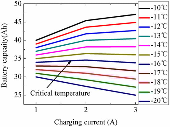
Figure 9.
Discharge curves of the lead-acid battery at low temperature.
Is is the solar charging current; Iw is the wind turbine charging current; IB is the charging current of battery, and IB is equal to the sum of Is and Iw; Ta is the ambient temperature; Tc is the critical temperature mentioned above (−16 °C). The charging strategy of the hybrid wind-solar system is shown in Table 5 and Table 6.
Table 5.
The charging strategy of the hybrid wind-solar system (Ta > Tc).
Table 6.
The charging strategy of the hybrid wind-solar system (Ta < Tc).
If Ta > Tc, there are three operating conditions for hybrid wind-solar system.
Operating condition 1 (the first and second rows of Table 5): In the polar day, the PV always works in MPPT mode. And if the value of wind speed is between Vc and VF, which means wind energy is available, the wind turbine also works in MPPT mode. Otherwise, wind energy cannot be utilized and the wind turbine does not work.
Operating condition 2 (the third and fourth rows of Table 5): In the polar night, the PV cannot work. At this time, if the wind energy is available, the wind turbine will work in MPPT mode. If the wind speed is below 3 m/s or above 40 m/s, the wind turbine does not work.
Operating condition 3: During normal daytime, the PV works in MPPT mode. And if the value of wind speed is between Vc and VF, the wind turbine also works in MPPT mode. Otherwise, the wind turbine does not work. In the night, the PV cannot work. At this time, if the wind energy is available, the wind turbine will work in MPPT mode. If the wind speed is below 3 m/s or above 40 m/s, the wind turbine does not work.
If Ta < Tc, a small current should be selected for battery charging. There are four operating conditions for hybrid wind-solar system.
Operating condition 4 (the first, second and third rows of Table 6): When it is in the polar day and the wind speed is between Vc and VF, if Is + Iw > Imax, the PV will work in MPPT mode and the wind turbine will enter current-limiting mode; if Is + Iw< Imax, the PV and wind turbine will all work in MPPT mode. And if Is > Imax, the PV will work in the current-limiting mode and the wind turbine will work in uploading mode to protect the system.
Operating condition 5 (the fourth and fifth rows of Table 6): When it is in the polar day and the wind speed is unavailable, the wind turbine cannot work. If Is > Imax, the PV will enter current-limiting mode; if Is ≤ Imax, the PV will enter MPPT mode.
Operating condition 6 (the sixth and seventh rows of Table 6): When it is in the polar night and the wind speed is available, the PV cannot work. If Iw > Imax, the wind turbine will work in current-limiting mode; if Iw ≤ Imax, the wind turbine will work in MPPT mode.
Operating condition 7 (the eighth row of Table 6): When it is in the polar night and the wind speed is unavailable, the PV and the wind turbine all cannot work and Is + Iw = 0.
4. Circuit Design
4.1. Charging Circuit
In the process of circuit design, we considered the impact of extremely cold environments of the Polar Region. Thus, low temperature characteristics and power consumption of the circuit devices must be examined in detail. The charging circuit consists of four parts: (1) the solar and SWT charging circuit, (2) the driver circuit, (3) the detection circuit and (4) ADC circuit and auxiliary circuit. The solar and SWT charging circuit is shown in Figure 10.
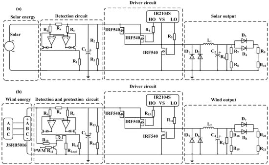
Figure 10.
Schematic of the solar circuit (a) and SWT charging circuit (b).
The solar charging circuit (Figure 10a) is a Buck circuit where C1 and C2 are electrolytic capacitors with values of 1000 μF; L1 is a toroidal inductor of 470 μH; the resistance values of R1, R4 and R5 are both 2 KΩ; the resistance value of R2 is 1 KΩ; the resistance value of R3 is 10 KΩ; and D1 and D2 are dual high-voltage Schottky rectifiers (MBR20H100CT, Vishay Semiconductors, TX, USA). The MOSFETs IRF540NPbF (International Rectifier, El Segundo, CA, USA) are selected for charging by controlling the on-off state.
The SWT charging circuit is shown in Figure 10b. The AC generated by the SWT is rectified to DC using 3SRB5016 (ASEMI, Ningbo, China), with an operating temperature range between −55 °C and 150 °C. An unloading circuit is designed in the SWT charging circuit to protect the SWT and charging circuit from damage when the wind speed in the polar region is too large and exceeds the limits of operation of SWT. C3 and C4 are electrolytic capacitors with values of 1000 μF, and L2 is a toroidal inductor of 470 μH. Under the condition that wind speed reaches the cut-in value, the MCU (MSP430F5438A, Texas Instruments, Dallas, TX, USA) can collect the voltage and current of the small WT via MPPT control strategy. MCU implements the MPPT strategy by changing the duty cycle of the PWM.
4.2. Driver Circuit
The main circuit of the solar and SWT charging circuit is the Buck circuit. The driver circuit is shown in Figure 11 and was developed by the IR2104S (International Rectifier, El Segundo, CA, USA).
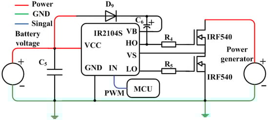
Figure 11.
Schematic of the driver circuit.
C5 is a capacitor with value of 100 nF. D9 is a low power-consumption Schottky diode SK34 (Diodes Incorporated, Plano, TX, USA), and C6 is a 1 μF tantalum capacitor that can be considered as a bootstrap capacitor. Current limiting resistors R23 and R24 are designed to have a resistance of 2 KΩ. The IN is connected to the PWM port of the MCU, and the LO has the same polarity as the pin IN, while the HO has the opposite polarity. The function of the drive circuit can be described as follows: After inputting the PWM at pin IN, (1) when the HO is low, the LO is high. At this time, the IRF540 connected to R24 is turned on and grounded, and the VCC is charged to C6 through D9, (2) When the HO is high, the LO is low. At this time, the VCC and the voltage of C6 are output from the HO, thereby controlling the turn-on and turn-off of the IRF540 connected to R23.
4.3. Detection Circuit
In the solar and SWT hybrid charging circuit, it is necessary to collect multiple sets of voltage and current data, such as the voltage of the wind turbine, the voltage of the solar cell, and the voltage of the battery. The collected current includes the charging current of the SWT and the charging current of the battery. The MAX471ESA (Maxim, San Jose, CA, USA) is selected as the core of the circuit during the design process. The MAX471 is a complete, bidirectional, high-side current-sense amplifier for portable battery monitoring, and operates at a temperature range between −40 °C and 85 °C.
4.4. ADC Circuit and Auxiliary Circuit
The ADS1100 (Texas Instruments, Dallas, TX, USA) was selected as the core of the ADC circuit. This circuit was assembled compatible with I2C serial interfaces, and has a simple circuit structure. The auxiliary circuit (Figure 12) contains two levels of voltage conversion: The primary and secondary voltage regulators. The primary voltage regulator (LT1129, Analog Devices Inc., Norwood, MA, USA) generates 3.3 V at supply of 12 V by a plurality of battery units. The secondary voltage regulator (LM2596, Texas Instruments, Dallas, TX, USA) generates 5 V at a supply of 12 V to fulfill the requirements of the iridium circuit.
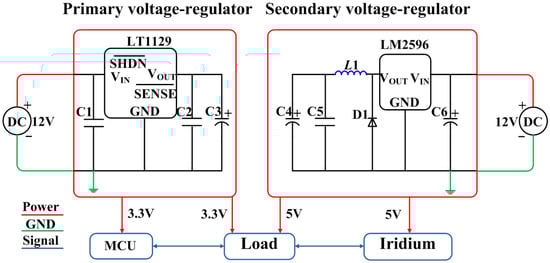
Figure 12.
Schematic of the auxiliary circuit.
5. Performance Evaluation of the Charging Circuit
In the Arctic Ocean or Antarctica, low temperatures are the primary challenge for the power supply of unmanned equipment. Our charging circuit and charging strategy may have been affected by instabilities of the components and modules. Although for the charging circuit components and modules were selected based on their good performance at low temperatures (−50–30 °C), the potential temperature dependence of the charging circuit had to be assessed. The temperature dependence of the detection and ADC circuits, which are important for the charging strategy, were evaluated and assessed.
5.1. Temperature Dependence of the Detection Circuit
We placed the detection circuit into the GDJS series high–low-temperature test chamber providing a stable environmental temperature over the range of −50 °C to 30 °C. The input voltage of the experiment was generated with programmable power-supply E3631A (Agilent, Santa Clara, CA, USA) to generate voltages from 2 V to 22 V. The output of the detection circuit was measured by an oscilloscope (MSO70404C, Tektronix, Beaverton, OR, USA). The interval of the experimental temperature was 20 °C. The interval of the measured voltage was set to 1 V. At each temperature, the high–low-temperature test chamber maintained the temperature for 20 min, during which measurements were repeated 300 times. We took the average values to minimize statistical error and uncertainty.
The output voltage and average error results are shown in Figure 13. The results demonstrate that the output of the detection circuit had a strong upward trend, proportional to the increase of input, and the temperature dependence of the detection circuit was within a narrow range. The R2 of the output of the detection circuit was greater than 0.99. The maximum average error of the output voltage of the detection circuit was 0.017 V at 10 V, and the minimum average error of the output voltage was −0.027 V at 6 V. Therefore, the experimental results show that the detection circuit has excellent stability at low temperatures, and can be used in the charging circuit for the polar regions.
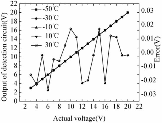
Figure 13.
Temperature dependence of the output of detection circuit and the average error.
5.2. Temperature Dependence of the ADC Circuit
In the temperature-dependence experiment of the ADC circuit, we also placed the ADC circuit into the high–low-temperature test chamber with the same temperature range. The input voltage of the ADC circuit was generated by a nominal 5 V voltage reference chip and a potentiometer with an input range from 1 to 3 V in intervals of 0.5 V. The results in Figure 14a demonstrate that the minimum value of the reference voltage was 3.302 V at −50 °C, maximum value was 3.308 V at −30 °C, average value of the output was 3.306 V, and standard deviation was 0.0015 V. We calculated the coefficient of variation of the reference voltage as 0.048%. The results in Figure 14b show that the five measured ADC outputs can be considered stable in a temperature range of −50–30 °C.
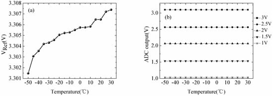
Figure 14.
Temperature dependence of the (a) reference voltage, and (b) output of the ADC circuit (the measured and ideal voltage values of 1, 1.5, 2, 2.5, and 3 V).
5.3. Temperature-Correction Algorithm for the Power System
As mentioned above, the evaluation reveals that the low-temperature performance of the detection circuit maintained a strong stability at a temperature range of −50–30 °C. However, we still developed an approach to correct and minimize deviation, because the accuracy of the detection circuit directly affects the operation effect of the charging strategy. The relationship between output current of the detection circuit ID(T) and corrected current Iout(T) could be approximated as follows:
where a(T), b(T), c(T), and d(T) are the coefficients of Equation (5).
We put the whole detection circuit into the GDJS series high–low-temperature test chamber over a range of −50–30 °C and measured the accuracy of the output current. During the experiment, the interval of the measured temperature was set as 5 °C from −50 °C to 30 °C. We measured the output of the detection circuit by the oscilloscope. Oscilloscope results were compared with the output current of the detection circuit. At each measured temperature, the high–low-temperature test chamber maintained the temperature for 20 min in which measurement was repeated 300 times. We took the average values to minimize statistical error and uncertainty. The coefficients a(T), b(T), c(T), and d(T) could be simultaneously calculated.
The results of measured currents of detection circuit and ideal currents are shown in Figure 15. We observe that the discrepancy between actual currents and measured values remained in the minimal range. The maximum and minimum errors were 0.0061 and 0.0015 A, respectively.
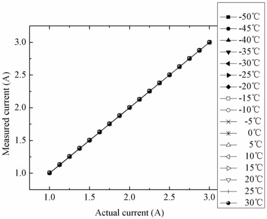
Figure 15.
Temperature dependence of the current of the detection circuit.
The coefficients a(T), b(T), c(T), and d(T) decreased approximately in a parabolic manner with increase of temperature (Figure 16). The maximum and minimum a(T) were −3.4 × 10⁻⁷ at 30 °C and −5.83 × 10⁻⁷ at −50 °C, respectively. The maximum and minimum values of b(T) were 1.28 × 10⁻⁵ at −50 °C and 7.47 × 10⁻⁷ at 30 °C, respectively. The maximum and minimum values of c(T) were 0.0298 at −50 °C and 0.0017 at 30 °C, respectively. The maximum and minimum values of d(T) were 0.211 at −50 °C and 0.012 at 30 °C, respectively. The value of coefficients a(T), b(T), c(T), and d(T) at the nonmeasured temperatures could be predicted by interpolation.
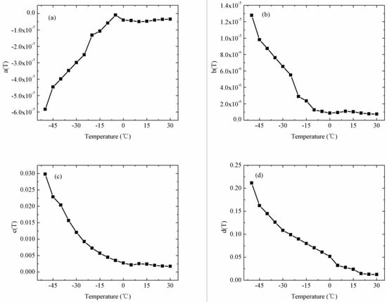
Figure 16.
(a–d) Temperature dependence of coefficients a, b, c, and d, respectively.
6. Results
6.1. Monthly Average Energy Production from the PV Panel and the WT
The monthly average PV and WT power generation near Zhongshan Station and monthly average load power are presented in Figure 17. Monthly average radiation-intensity, wind-speed, and air-temperature data were obtained from NASA’s atmospheric science data center. It can be noted that wind-power production dominated the power supply and generated 66.07 KWh in a year. The monthly average maximum (minimum) value of wind power was 7.11 KWh (3.13 KWh) in August (January). Solar power showed strong seasonal fluctuations because of the polar night in June and July. The monthly average solar power of the polar day in January and December was larger at 2.90 and 3.21 KWh, respectively. The minimum value of the monthly average solar power in a year appeared in June and July, which was during the polar night in Antarctica. In contrast, wind energy was considered to be significant from May to August. The power generation of the PV and WT in Zhongshan Station showed good monthly characteristics. Monthly load demands of the observing system were basically the same. The maximum and minimum load demands were 3.11 KWh in June and 3.56 KWh in January, March, May, August, October, and December, respectively. The minimum power output of the power-supply system was 5.35 KWh in February, which can satisfy the power demands of the observing system in normal operation.
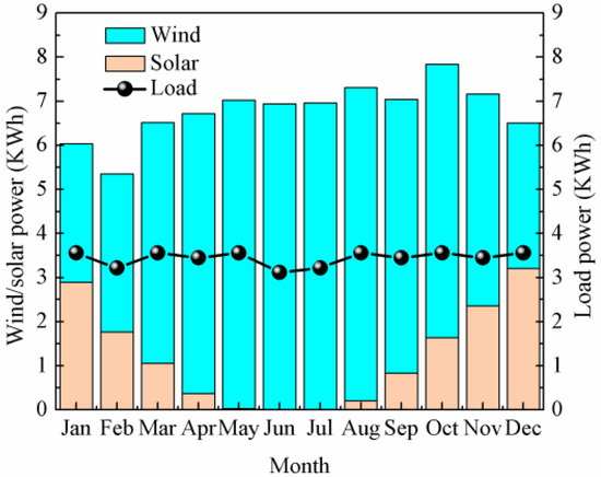
Figure 17.
Monthly average PV and WT energy power production and load demand of the observing system in Zhongshan Station, Antarctica.
6.2. Case Study in Antarctica
The new observing system was deployed in the station area of Zhongshan Station on 6 February 2017 during the 2016 Chinese National Antarctica Research Expedition. The observing system observed the meteorological data and ice mass balance data from 6 February 2017 to 9 July 2017. The hybrid solar and SWT charging circuit were also assembled during the operation of the observing system. The air-temperature distribution measured by the observing system in Zhongshan Station from 6 February 2017 to 9 July 2017 is presented in Figure 18. The sampling interval of the air temperature was one hour. In Figure 17, we can see that the minimum air temperature was −41.375 °C on 6 July 2017, which was in the period of the polar night. The maximum air temperature was −4.625 °C on 18 February 2017, which was in the period of the polar day. The average temperature from 6 February 2017 to 9 July 2017 was −23.94 °C. Temperature distribution was below 0 °C, in line with our expectations and the temperature range of the observing and power-supply systems.

Figure 18.
Daily air temperature measured by the observing system from 6 February 2017 to 9 July 2017 in Zhongshan Station, Antarctica. The area between the red lines is the polar night.
Figure 19 shows the daily radiation intensity and solar power from 6 February 2017 to 9 July 2017, respectively. Overall, radiation intensity continued to decline from 6 February 2017 (Figure 19a). Then, from 27 May to 9 July, radiation intensity was 0 W/m2, which was during the polar night. Although the observation system was initially deployed during the polar day, the intraday variation of radiation intensity was more severe. The minimum value of radiation intensity was 0 W/m2 in the period of polar night. Maximum radiation intensity was 1073 W/m2 on 10 February 2017, which was in the period of the polar day. The average radiation intensity from 6 February 2017 to 9 July 2017 was 114 W/m2.
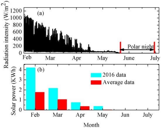
Figure 19.
(a,b) Daily radiation intensity measured by the observing system, and solar power generated by the power system from 6 February 2017 to 9 July 2017, respectively. Area between the red lines is the polar night.
In Figure 19b, the trends of solar power and radiation intensity were considered to be gradually reduced. The minimum value of solar power was 0 KWh in the period of the polar night (June and July). Maximum solar power was 4.2 KWh on 10 February 2017, which was in the period of the polar day. The average solar power from February to July 2017 was 1.25 KWh. The trend of calculated solar power based on the radiation-intensity data obtained in 2017 was consistent with the calculation using average data from NASA, except for solar power in January. The particularity of the installation location of the observing system may cause differences in the calculated values between measured and average data.
The wind speed and monthly wind power are shown in Figure 20, respectively. As shown in Figure 20a, the minimum value of wind speed was 0 m/s, and the maximum wind speed was 69.7 m/s on 7 March 2017. Average wind speed from 6 February 2017 to 9 July 2017 was 22.7 m/s (Figure 20a). The 93.5% of wind energy can be used to generate electricity using the power system (dark-blue area in Figure 19a). In Figure 20b, the difference between actual wind-power generation and calculated wind power was in a small range, except that the maximum wind power was 13.46 KWh in April, which was about twice the calculated wind power. Since the deployment of the observation system was until 9 July 2017, the wind energy of the current month was much smaller than the wind power calculated by average data.
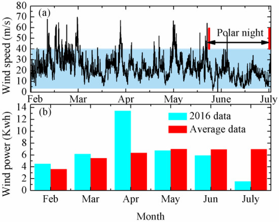
Figure 20.
(a) Wind speed measured by the observing system, and (b) monthly wind power generated by the power system and calculated by the average data from 6 February 2017 to 9 July 2017, respectively. Area between the red lines is the polar night. The dark-blue area represents the available wind.
The power supply of the observing system is shown in Figure 21. The supply-voltage range required for the observing system to operate normally is from 13 to 20 V. As shown in Figure 21, the voltage of the output of the power system continued to decline from February to July. From the date of deployment to the end of April, the voltage was a fluctuant downward trend owing to the superposition of solar and wind energy. After that, radiation intensity was reduced until it was 0 W/m2 in the polar night, during which wind power was alone as a source of energy. In the operating cycle of the observation system in Antarctica, supply voltage was always higher than 13 V, that is, the power-supply system could guarantee the operation of the observation system in the range of −50–30 °C.
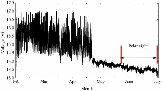
Figure 21.
Power voltage of the observing system. Area between the red lines is the polar night.
7. Conclusions
In this study, we proposed a standalone hybrid wind–solar system for the polar regions. The operation of the observation system in the Arctic Ocean in 2016 and the meteorological environment of the deployment positions were analyzed. A new observation system and a power-supply system with a hybrid solar and wind charging circuit were designed to achieve long-term stable operation in the polar regions at a temperature range of −50–30 °C. We presented a comprehensive understanding of the low-temperature performance and characteristics of batteries, including battery capacity at different temperatures, and the charging characteristics of the lead–acid battery. Based on the low-temperature characteristics of the battery, a charging strategy adapted for the battery was proposed. We evaluated the low-temperature performances of the charging circuit to implement charging strategy. The detection and ADC circuits of the charging circuit have excellent stabilities in the range of −50–30 °C. The simulation calculation of power generation of the standalone hybrid wind–solar system was presented in this study. The results of the simulation calculation reveal that wind power had a relatively higher share of energy production than the PV. The observing system and the standalone hybrid wind–solar system were applied to the observation of ice-matter balance in Zhongshan Station, East Antarctica from February to July 2017. The power generation of the PV and wind turbine during the field experiment was calculated. The case study shows that the standalone hybrid wind–solar system can be proven to have high stability, and also indicates that our study on battery characteristics in low-temperature environments could greatly improve battery reliability. This paper demonstrates that the standalone hybrid solar–wind system is an ideal solution for automatic observation systems in the polar regions.
In this study, the standalone hybrid solar–wind system does not emit any pollutants during its lifecycle. However, lead–acid batteries were used as energy-storage units for the power system. Although we designed a leak-proof container to place small batteries to avoid polluting the environment, more environmentally friendly energy storage unit needs to be adopted in future work. More renewable energy, such as wave energy, temperature-difference energy, and salinity-difference energy, in the polar region can be used to design power-supply systems with larger installed capacity.
Author Contributions
conceptualization, G.Z.; methodology, G.Z.; software, G.Z.; validation, G.Z.; formal analysis, Y.D.; investigation, Y.C.; writing—original draft preparation, G.Z.; funding acquisition, Y.D., X.C., and Y.C.
Funding
This research was funded by the National Natural Science Foundation of China, grant number 41606220, 41776199; the National Key Research and Development Program of China, grant number 2016YFC1402702, 2016YFC1400303; and the Natural Science Foundation of Shanxi, grant number 201701D121127.
Acknowledgments
The authors would like to thank the Chinese National Arctic Research Expeditions and Chinese National Antarctica Research Expeditions for supporting the deployment of the observing and power-supply systems. Comments from the anonymous reviewers and the editor are also gratefully appreciated.
Conflicts of Interest
The authors declare no conflict of interest.
References
- Rothrock, D.A.; Percival, D.B.; Wensnahan, M. The decline in arctic sea-ice thickness: Separating the spatial, annual, and interannual variability in a quarter century of submarine data. J. Geophys. Res. Oceans 2008, 113, C05003. [Google Scholar] [CrossRef]
- Perovich, D.K.; Grenfell, T.C.; Light, B. Transpolar observations of the morphological properties of Arctic sea ice. J. Geophys. Res. 2009, 114, C00A04. [Google Scholar] [CrossRef]
- Haas, C.; Hendricks, S.; Eicken, H. Synoptic airborne thickness surveys reveal state of Arctic sea ice cover. Geophys. Res. Lett. 2010, 37. [Google Scholar] [CrossRef]
- Haas, C.; Pfaffling, A.; Hendricks, S. Reduced ice thickness in Arctic Transpolar Drift favours rapid ice retreat. Geophys. Res. Lett. 2008, 35, L17501. [Google Scholar] [CrossRef]
- Rack, W.; Haas, C.; Langhorne, P. Airborne thickness and freeboard measurements over the McMurdo Ice Shelf, Antarctica, and implications for ice density. J. Geophys. Res. Oceans 2013. [Google Scholar] [CrossRef]
- Richter-Menge, J.A.; Perovich, D.K.; Elder, B. Ice mass balance buoys: A tool for measuring and attributing changes in the thickness of the Arctic sea ice cover. Ann. Glaciol. 2006, 44, 205–210. [Google Scholar] [CrossRef]
- Jackson, K.; Wilkinson, J.; Maksym, T. A novel and low cost sea ice mass balance buoy. J. Atmos. Ocean. Technol. 2013, 30, 13825. [Google Scholar] [CrossRef]
- Wang, H.Z.; Chen, Y.; Song, H. A Fiber Optic Spectrometry System for Measuring Irradiance Distributions in Sea Ice Environment. Atmos. Ocean. Technol. 2014, 31, 2844. [Google Scholar] [CrossRef]
- Lei, R.B.; Li, N.; Heil, P. Multiyear sea ice thermal regimes and oceanic heat flux derived from an ice mass balance buoy in the Arctic Ocean. J. Geophys. Res. Oceans 2014, 119, 537–547. [Google Scholar] [CrossRef]
- Lei, R.B.; Cheng, B.; Heil, P. Seasonal and Interannual Variations of Sea Ice Mass Balance From the Central Arctic to the Greenland Sea. J. Geophys. Res. Oceans 2018. [Google Scholar] [CrossRef]
- Borowy, B.S.; Salameh, Z.M. Optimum photovoltaic array size for a hybrid wind/PV system. IEEE Trans. Energy Convers. 1994, 9, 482–488. [Google Scholar] [CrossRef]
- Deshmukh, M.K.; Deshmukh, S.S. Modeling of hybrid renewable energy systems. Renew. Sustain. Energy Rev. 2008, 12, 235–249. [Google Scholar] [CrossRef]
- Bilal, B.O.; Sambou, V.; Ndiaya, P.A. Optimal design of a hybrid solar–wind-battery system using the minimization of the annualized cost system and the minimization of the loss of power supply probability (LPSP). Renew. Energy 2010, 35, 2388–2390. [Google Scholar] [CrossRef]
- Diaf, S.; Diaf, D.; Belhamel, M. A methodology for optimal sizing of autonomous hybrid PV/wind system. Energy Policy 2007, 35, 1303–1307. [Google Scholar] [CrossRef]
- Dihrab, S.S.; Sopian, K. Electricity generation of hybrid PV/wind systems in Iraq. Renew. Energy 2010, 35, 1303–1307. [Google Scholar] [CrossRef]
- Ghoddami, H.; Delghavi, M.B.; Yazdain, A. An integrated wind-photovoltaic-battery system with reduced power-electronic interface and fast control for grid-tied and off-grid applications. Renew. Energy 2012, 45, 128–137. [Google Scholar] [CrossRef]
- Sreeraj, E.S.; Chatterjee, K.; Bandyopadhyay, S. Design of isolated renewable hybrid power systems. Sol. Energy 2010, 84, 1124–1136. [Google Scholar] [CrossRef]
- Gunasekaran, M.; Ismail, H.M.; Chokkalingam, B. Energy Management Strategy for Rural Communities’ DC Micro Grid Power System Structure with Maximum Penetration of Renewable Energy Sources. Appl. Sci. 2018, 8, 585–608. [Google Scholar] [CrossRef]
- Vasiliev, M.; Alameh, K.; Nur-E-Alam, M. Spectrally-Selective Energy-Harvesting Solar Windows for Public Infrastructure Applications. Appl. Sci. 2018, 8, 849–864. [Google Scholar] [CrossRef]
- Kadir, A.E.; Hu, A.P. A Power Processing Circuit for Indoor Wi-Fi Energy Harvesting for Ultra-Low Power Wireless Sensors. Appl. Sci. 2017, 7, 827–845. [Google Scholar] [CrossRef]
- Ma, T.; Yang, Y.X.; Lu, L. Technical feasibility study on a standalone hybrid solar-wind system with pumped hydro storage for a remote island in Hong Kong. Renew. Energy 2014, 69, 7–15. [Google Scholar] [CrossRef]


© 2018 by the authors. Licensee MDPI, Basel, Switzerland. This article is an open access article distributed under the terms and conditions of the Creative Commons Attribution (CC BY) license (http://creativecommons.org/licenses/by/4.0/).