Parameter Optimization Method for Identifying the Optimal Nonlinear Parameters of a Miniature Transducer with a Metal Membrane

Abstract

This study proposes a parameter optimization method for identifying the optimal nonlinear parameters of a miniature transducer with a metal membrane. Specifically, a nonlinear lumped parameter model (LPM) of a miniature transducer that accounts for predicted displacement in a manner that is consistent with the displacement measured by a high-precision capacitance micro-displacement sensor is proposed. To avoid application of the proposed optimization method to an ill-posed problem, this paper proposes a constrained equation that is derived from the relationships of nonlinear parameters. The Broyden–Fletcher–Goldfarb–Shanno (BFGS) algorithm is used to minimize the objective function in order to obtain an appropriate solution from the proposed nonlinear LPM. The numerical simulation results and a discussion of the experiments are presented. The numerical simulation verification demonstrated that the presented method can estimate the suitable nonlinear parameters for the displacement with errors. With regard to empirical verification, the empirical investigations showed that the proposed method could accurately assess the nonlinear parameters of a miniature transducer with a metal membrane.

1. Introduction

The nonlinear parameters of a miniature transducer play an important role in the sound quality of mobile devices. These parameters can be responsible for the output performance of a miniature transducer. Special techniques can be used to measure the harmonic and intermodulation distortion of signals excited by single-, dual-, and multi-tone sine waves/signals. In the last decade of research on transducers, multiple methods have been proposed to predict harmonic and intermodulation distortion, and these methods are useful in transducer design. The traditional method used to predict the sound pressure, diaphragm displacement, and electric current of a moving-coil transducer comprise the lumped parameter model (LPM) [1], which allows for the comprehensive analysis of a transducer’s model parameters. The traditional LPM contains an important set of six parameters, namely, voice-coil inductance L_e, electrical resistance R_e, mechanical mass M_m, mechanical resistance R_m, mechanical stiffness K_m, and force factor Bl, which are used to represent the electrical and mechanical domains of the moving-coil transducer. The LPM helps to design a transducer quickly and accurately to estimate its performance, and it is currently the most common method used to assess the transducer quality.

Electroacoustic measurement is characterized by multiple categories and methods [2]. Each measurement provider formulates different instruments and procedures for transducers with different dimensions. Different methods have been applied by scientists in the past, such as the added mass method [1,3] and the optimization method [4], for transducer’s linear parameters estimation. When the miniature transducer is driven in the large signal domain, abnormal vibrations have been observed due to large input signal and increased voltage imposed on voice coil for its displacement [5]. The moving diaphragm that was activated by pneumatic pressure [6] demonstrated that the transducer’s model parameters cannot remain linear, but the performance of the transducer can be evaluated by position-dependent parameters [7] as nonlinear parameters. In 1990, Klippel [8] proposed a dynamic measurement system and used a high-precision laser vibrometry and noise signal to measure the linear and nonlinear parameters of a transducer LPM. The nonlinear parameters generate nonlinear effects, such as harmonic and intermodulation distortion; thus, the system that was proposed by Klippel is often used for transducer development, production, quality control, and diagnostics [5,9]. Faifer et al. [10] proposed a nonlinear LPM to identify the coefficient of stiffness K_m(x) and the force factor (Bl) and investigated the reduction of 2nd–3rd harmonic distortions by transducer parameter linearization. A simulation method [11] uses finite element analysis for the identification of the nonlinear parameters early, which is the meaningful way of characterizing the transducer in the product development process. In 2001, Mihelich proposed [12] a parameter optimization method for minimizing the cost function between the predicted sinusoid type of displacements and the modeled response for obtaining nonlinear parameters. More proposed algorithms [13,14] based on the system identification method are used to minimize the errors between the output response and the system output for obtaining optimal nonlinear parameters. However, the relative clay mass or sealed box were selected based on the transducer dimensions, thus the above methods increased the mechanical mass or acoustical stiffness of the transducer, which are not applicable to miniature and small transducers.

Modern miniature transducers have been developed as part of the trend toward the miniaturization and they have been fabricated with metal membranes due to the low weights and dynamic responses. The displacement measurement errors caused by diaphragm vibration in a miniature transducer with a metal membrane may encounter errors due to optical refraction during laser measurements. Hence, there is the need to increase diaphragm reflection accuracy by making a mark on the diaphragm. The measurement of displacement is the basis of measuring position, velocity, acceleration, stress, force, pressure, proximity, thickness, etc. A displacement sensor measures the distance between the sensor and an object to be detected by identifying the displacement over a variety of elements and converting it into a distance. In 2012, Lei et al. [15] proposed a quartz crystal capacitive sensor that consists of a uniplanar scattering-field capacitance and a piezoelectric resonator for high sensitivity response (3.05 Hz/μm in the range of 20–200 μm). In the same year, Kang et al. [16] proposed a low-power high-resolution capacitive sensor for fast vibration measurements. As shown in the studies that were reviewed above, the high precision and better resolution of capacitive sensor testing were the main reasons for measuring the diaphragm displacement of a miniature transducer with a composite metal membrane in this study.

To identify the nonlinear parameters, among the conventional optimization methods for parameter estimation, such as the Stochastic Gradient Descent (SGM) [17], RMSProp and ADAM [18], Conjugate Gradient method (CGM) [19], and Broyden Fletcher Goldfarb Shanno Method (BFGS) [20], are the incremental gradient descent based iterative method for optimizing a differentiable objective function. The gradient descent algorithm updates the optimized parameters to minimize the objective function by taking small learning steps in the direction of the negative gradient of the loss of the objective function. The CGM searches from the conjugate direction along the negative gradient with the characteristics of double convergence from SGM; moreover, SGM and CGM use a single learning rate for all of the parameters. The RMSProp can improve by using learning steps that are different for different parameters and that can automatically adapt to the objective function being optimized. The BFGS method is one of the famous methods that belongs to quasi-Newton methods [20], which uses an estimation to the inverse Hessian matrix to guide its search through variable space. BFGS generally requires much fewer iterations to reach the local minimum as compared to CGM and SGM. In this paper, the miniature transducer’s differential equation was established and the use of the Broyden–Fletcher–Goldfarb–Shanno (BFGS) algorithm [20] to identify the nonlinear parameters simultaneously during the optimization process was proposed in this study. The Brent method [21] was also utilized to improve the step size for accelerating iteration times. The transducer’s equation of impedance curve as a constraint in order to ensure the correctness of optimization parameters and their correspondence with the miniature transducers’ physical conditions was used. In order to account for measurement errors in the transducer’s displacement, the distribution function with different standard deviations was used to simulate the measurement errors for verifying the results. The experiment system that was employed in this study utilized a high-precision capacitive micro-displacement sensor to measure the diaphragm displacement x(t). A high-precision electric current instrument was used to measure the transducer’s electric current i(t). In the results and discussion sections, the numerical simulation tests and experiments are both discussed in detail.

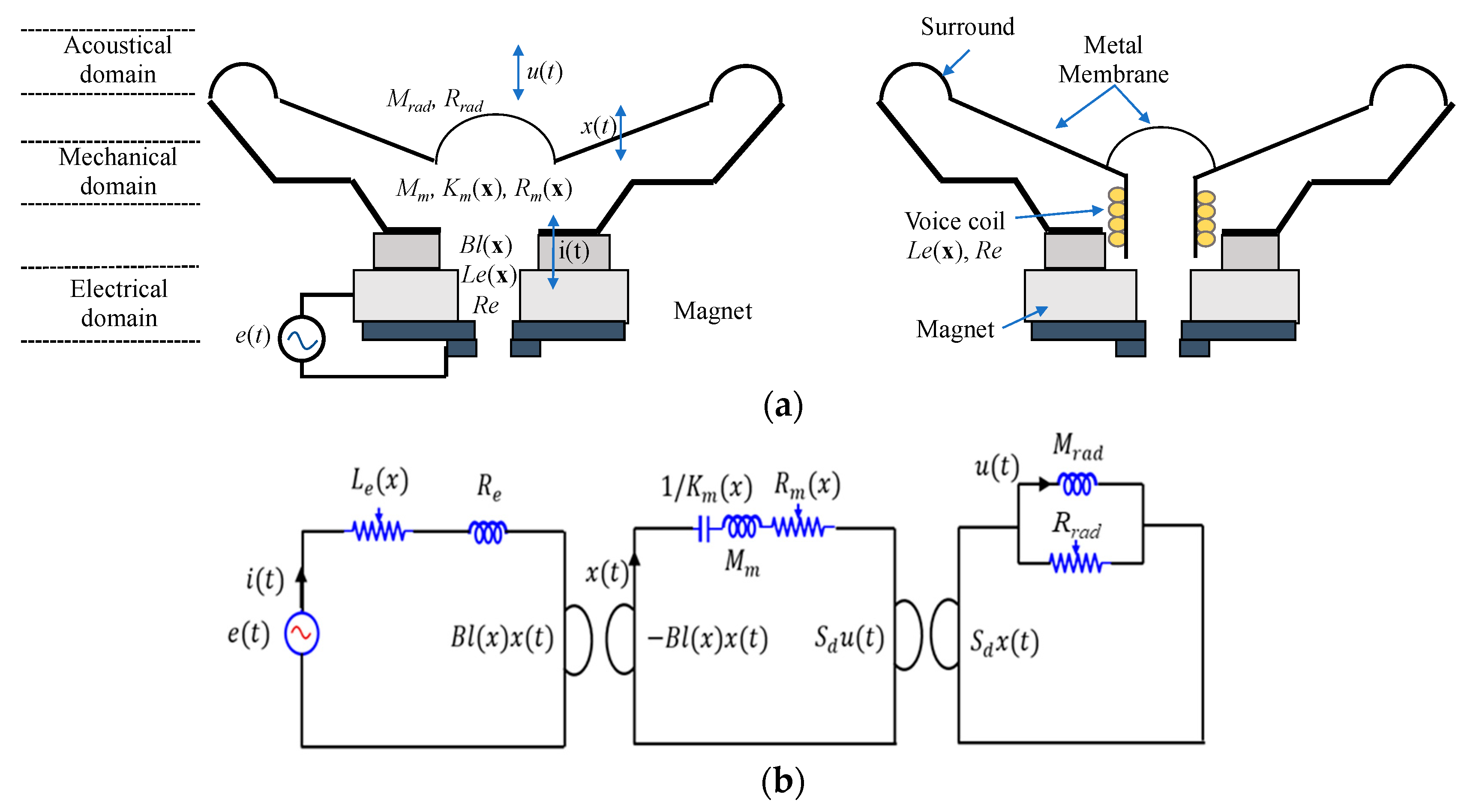
2. Mathematical Model

2.1. Transmission Equation

The suspension system of a miniature transducer comprises a surround and a diaphragm. The behaviors of these two parts are described by the mechanical mass, stiffness, and damping. The nonlinear vibration characteristics of the suspension and the magnetic system occur with the instantaneous excursion of voice-coil displacement from the mean position. To represent this nonlinear vibration characteristics in modeling, the nonlinear parameter K_m(x) as a form of the non-linear mechanical stiffness is used to describe the nonlinear vibration characteristics [8]. The parameters K_m(x) and R_m(x) indicate that the change in the value of the mechanical stiffness depends on the displacement x, while L_e(x) represents the voice-coil inductance of the magnetic system, and Bl(x) represents the nonlinearity in the energy transfer between the electrical and mechanical domains. Figure 1a shows a schematic representation of the miniature transducer under large-signal conditions:

The equivalent circuit of an electrical domain (Figure 1b) can be derived based on Kirchhoff’s voltage law (Equation (1)):

$$L_e(x)\frac{di(t)}{dt}+\left[\frac{d{L}_e(x)}{dx}\frac{dx(t)}{dt}+R_e\right]i(t)+Bl(x)\frac{dx(t)}{dt}=e(t)$$

(1)

where e(t) is the input voltage; i(t) is the voice coil current; and, x(t) is the voice coil displacement. Nonlinear parameters include voice coil inductance L_e(x) and the force factor Bl(x). With regard to the mechanical domain, Newton’s second law of motion can be used to derive the current, as shown in the following equation:

$$M_m\frac{d^{2}x(t)}{d{t}^2}+R_m(x)\frac{dx(t)}{dt}+K_m(x)x(t)=\left(Bl(x)-\frac{d{L}_e(x)}{dx}\frac{i(t)}{2}\right)i(t)$$

(2)

where M_m is the mass of transducer diaphragm; R_m(x) is the damping coefficient of the suspension system; and, K_m(x) is the nonlinear coefficient of the stiffness of the suspension system. All nonlinear parameters, including K_m(x), R_m(x), Bl(x), and L_e(x), are related to displacement x. In the air load system model, the mass M_m in Equation (2) includes the mechanical mass of the diaphragm and voice coil. The interaction of air load mass M_rad and resistance R_rad in acoustic radiations must be also considered [1]. Therefore, the air load in the mechanical and acoustic fields is given, as follows:

$$\left(Bl(x)+\frac{d{L}_e(x)}{dx}\frac{i(t)}{2}\right)i(t)=\left(M_m+M_{rad}{S}_d\right)\ddot{x}(t)+R_m(x)\dot{x}(t)+K_m(x)x(t)$$

(3)

$$M_{rad}u\left(\mathrm{t}\right)=R_{rad}\left[S_d\dot{x}(t)-u\left(\mathrm{t}\right)\right]$$

(4)

Under the initial conditions:

$$x(0)=0,i(0)=0,u(0)=0,\mathrm{and}{\frac{dx(t)}{dt}|}_{t=0}=0$$

(5)

where S_d is the diaphragm area. The u(t) is the shunt volume velocity related to the acoustic radiation mass M_rad and the acoustic radiation resistance R_rad in Equation (4).

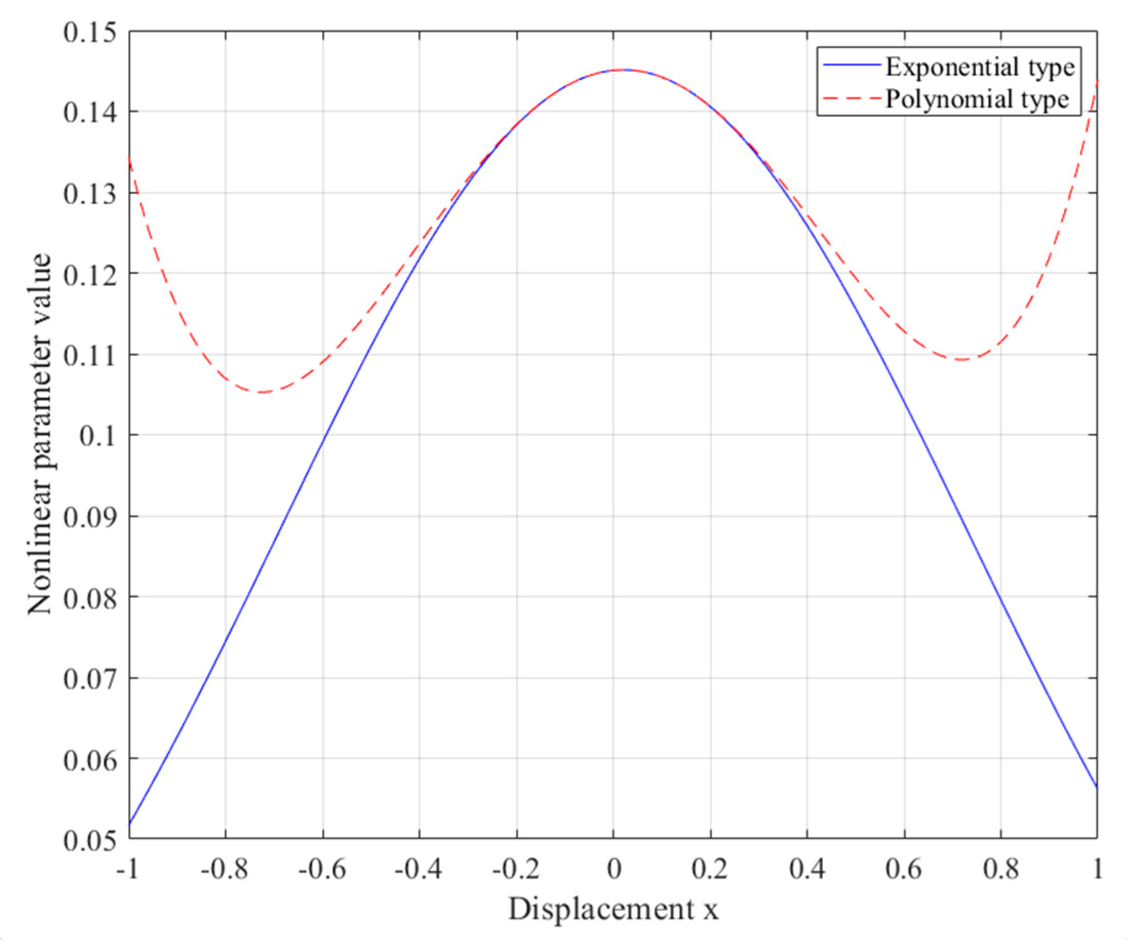
2.2. Nonlinear Parameter Fitting Equations

The nonlinear parameters R_m(x), Bl(x), K_m(x), and L_e(x) describe variations along the axial direction of the displacement x of the membrane. According to refs. [12,22], these nonlinear parameters can be approximated based on the polynomial power series function. The polynomial function is shown in Equation (6):

$$A(x)={\displaystyle \sum _{j=0}^N{A}_j{x}^j}=A_0+A_{1}x+A_2{x}^2+\dots +A_N{x}^N$$

(6)

where j represents the index of summation; A_j in general may represent force factor, coefficient of mechanical stiffness, and voice coil inductance, depending on the nonlinear parameter under consideration; and, N is the upper bound of summation. The exponential approximation coefficients can also be used to fit the nonlinear parameters. The exponential fitting equation can be defined, as follows:

$$A(x)=A_1\exp \left(\frac{\pm {(x-A_2)}^2}{A_3{}^2}\right)$$

(7)

where the coefficient A₁, A₂, and A₃ are the expected parameters of the nonlinear distribution and they can demonstrate the nonlinear parameters versus the displacement values. In this paper, the polynomial function was replaced with the exponential fitting function to reduce the measurement errors. As shown in Figure 2, when the polynomial equation was used to determine the nonlinear parameters, the increased displacement of the nonlinear parameters could cause an error in the parameter curve.

If the x(0) parameter and initial condition are known (normally set to 0), the voice coil displacement x(t) and electric current i(t) in Equations (1)–(5) are direct solutions. In contrast, for any time interval $t\in (0,t_f)$, if the input voltage is e(t), the voice coil displacement is x(t) and the voice coil current is i(t), then the solutions to the unknown coefficients in Equations (1)–(4) become optimal solutions. This study is aimed to determine all of the parameters described in the following section.

2.3. Calculation of Nonlinear Optimization Parameters

In order to obtain parameters by the proposed method, estimated and measured values of diaphragm displacement were used to define the target function J.

$$J(w)=J_1(w)+J_2(w)={\displaystyle {\int }_0^{t_f}{\left[x(t;w)-x_{mea}(t)\right]}^{2}dt}+\mu {\displaystyle {\int }_0^{t_f}{\left[i(t;w)-i_{mea}(t)\right]}^{2}dt}$$

(8)

where the unknown vector w = [M_m, R_m(x), Bl(x), K_m(x), L_e(x)] is the unknown nonlinear parameter that needs to be determined; x(t;w) is the estimated displacement; x_mea(t) is the measured displacement using a precise displacement sensor; i(t;w) is the estimated current; i_mea(t) is the measured current; and, $\mu$ is the weight coefficient of the difference between J₁(w) and J₂(w). The equation shows that when the target function J(w) reaches the minimum value, the estimated value x(t) approaches the measured value x_mea(t). Moreover, when the unknown coefficients of the vector w approach its extreme value, a positive solution can be reached for w. The parameter w can be adjusted, as follows:

$$w_{(\mathrm{n}+1)}^{}=w_{\left(\mathrm{n}\right)}-{\beta }_{\left(\mathrm{n}\right)}{P}_{\left(\mathrm{n}\right)}$$

(9)

where n represents the nth iteration; ${\beta }_{\left(\mathrm{n}\right)}$ represents the nth step; and P_(n) is the nth direction with decreasing values of unknown parameter vector.

2.4. Broyden–Fletcher–Goldfarb–Shanno (BFGS) Algorithm

The BFGS method [20] is an unrestricted optimization method that has been recently acknowledged as the most effective algorithm for solving unrestricted nonlinear optimization problems by the iterative method. The BFGS method was used to adjust the $P_{\left(\mathrm{n}\right)}$ value in the following manner:

$$P_{\left(\mathrm{n}\right)}=-\left(\nabla J_{\left(\mathrm{n}\right)}{A}_{\left(\mathrm{n}\right)}\right)=-\left({\left(\frac{\partial J}{\partial w}\right)}_{\left(\mathrm{n}\right)}{A}_{\left(\mathrm{n}\right)}\right)$$

(10)

$$A_{\left(\mathrm{n}\right)}=A_{(\mathrm{n}-1)}+E_{(\mathrm{n}-1)}$$

(11)

$$\begin{array}{ll}{E}_{\left(\mathrm{n}\right)}=& \frac{1}{{(\Delta w_{\left(\mathrm{n}\right)})}^T\Delta g_{\left(\mathrm{n}\right)}}\times \\ & \left[(\Delta w_{\left(\mathrm{n}\right)}{}^T\Delta w_{\left(\mathrm{n}\right)})\left(1+\frac{{(\Delta g_{\left(\mathrm{n}\right)})}^T{A}_{\left(\mathrm{n}\right)}\Delta g_{\left(\mathrm{n}\right)}}{\Delta w\Delta g_{\left(\mathrm{n}\right)}}\right)-A_{\left(\mathrm{n}\right)}\Delta g_{\left(\mathrm{n}\right)}{(\Delta x_{\left(\mathrm{n}\right)})}^T-\Delta x_{\left(\mathrm{n}\right)}{(\Delta g_{\left(\mathrm{n}\right)})}^T{A}_{\left(\mathrm{n}\right)}\right]\end{array}$$

(12)

where $A_{\left(0\right)}=I$ is the identity matrix. $\Delta w_{\left(\mathrm{n}\right)}=w_{\left(\mathrm{n}\right)}-w_{(\mathrm{n}-1)}$ and $\Delta g_{\left(\mathrm{n}\right)}=g_{\left(\mathrm{n}\right)}-g_{(\mathrm{n}-1)}$ are the differences between iteration values and $g_{(\mathrm{n})}=\nabla J{(w)}_{(\mathrm{n})}$ is the gradient function, which can be calculated, as follows:

$$\nabla J{(w)}_{(\mathrm{n})}={\left(\frac{\partial J}{\partial w}\right)}_{(\mathrm{n})}={\left(\frac{\partial J}{\partial M_m},{\left[\frac{\partial J}{\partial A_N^{Bl}}\right]}_{N_{Bl(x)}},{\left[\frac{\partial J}{\partial A_N^{K_m}}\right]}_{N_{K_m(x)}},{\left[\frac{\partial J}{\partial A_N^{R_m}}\right]}_{N_{R_m(x)}},{\left[\frac{\partial J}{\partial A_N^{L_e}}\right]}_{N_{L_e(x)}}\right)}_{(\mathrm{n})}$$

(13)

where $\partial J/\partial w$ is the Jacobian matrix of the target function J(w), it can be obtained by using the forward difference method, as follows:

$${\left(\frac{\partial J}{\partial w}\right)}_{(\mathrm{n})}=\left(\frac{x(t;w+\Delta h)-x(t;w)}{\Delta h}+\frac{i(t;w+\Delta h)-i(t;w)}{\Delta h}\right)$$

(14)

where $\Delta h$ is set to a small number as $1\times {10}^{-8}$ to get the approximation of $g_{(n)}$.

After determination of the search direction P_(n) and w minor deviation, a corresponding minor deviation $\Delta x(t;w)$ is produced for displacement $x(t;w)$. Thus, substituting $\Delta x(t;w)$ and $\Delta i(t;w)$ into Equation (8) leads:

$$\begin{array}{l}J{(w)}_{(\mathrm{n}+1)}={\displaystyle {\int }_0^{t_f}{\left[x(t;w_{\left(\mathrm{n}\right)}-{\beta }_1{}_{\left(\mathrm{n}\right)}{P}_{\left(\mathrm{n}\right)})-x_{mea}(t)\right]}^{2}dt+}\mu {\displaystyle {\int }_0^{t_f}{\left[i(t;w_{\left(\mathrm{n}\right)}-{\beta }_2{}_{\left(\mathrm{n}\right)}{P}_{\left(\mathrm{n}\right)})-i_{mea}(t)\right]}^{2}dt}\\ ={\displaystyle {\int }_0^{t_f}{\left[x(t;w_{\left(\mathrm{n}\right)})-{\beta }_1{}_{\left(\mathrm{n}\right)}\Delta x(t;P_{\left(\mathrm{n}\right)})-x_{mea}(t)\right]}^{2}dt+}\mu {\displaystyle {\int }_0^{t_f}{\left[i(t;w_{\left(\mathrm{n}\right)})-{\beta }_2{}_{\left(\mathrm{n}\right)}\Delta i(t;P_{\left(\mathrm{n}\right)})-i_{mea}(t)\right]}^{2}dt}\end{array}$$

(15)

When $J{(w)}_{(\mathrm{n}+1)}$ approaches 0, Equation (15) can be applied:

$${\beta }_{\left(\mathrm{n}\right)}={\beta }_1{}_{\left(\mathrm{n}\right)}+{\beta }_2{}_{\left(\mathrm{n}\right)}=\frac{{\displaystyle {\int }_0^{t_f}\left(x(t;w)-x_{mea}(t)\right)\Delta x(t;w)dt}}{{\displaystyle {\int }_0^{t_f}\Delta x{(t;w)}^{2}dt}}+\mu \frac{{\displaystyle {\int }_0^{t_f}\left(i(t;w)-i_{mea}(t)\right)\Delta i(t;w)dt}}{{\displaystyle {\int }_0^{t_f}\Delta i{(t;w)}^{2}dt}}$$

(16)

where $\Delta x(t;w)$ and $\Delta i(t;w)$ can be used to conduct direct numerical differentiation of $x_{(\mathrm{n}+1)}-x_{\left(\mathrm{n}\right)}/(\Delta k\Vert x\Vert )$ and $i_{(\mathrm{n}+1)}-i_{\left(\mathrm{n}\right)}/(\Delta k\Vert i\Vert )$, respectively. In this study, $\Delta k$ was the extreme value $1\times {10}^{-8}$, which is set for displacement x.

2.5. Brent’s Algorithm

As the target function approaches the minimum value with each iteration, deviations could occur with respect to the step value ${\beta }_{\left(\mathrm{n}\right)}$ that was obtained from Equation (16). In order to obtain the optimal step values in the iteration direction, Brent’s algorithm [21] was used to derive the approximate optimal value ${\beta }_{\left(\mathrm{n}\right)}$. With regard to the numerical analysis, Brent’s method is a complex but widely used root-finding algorithm that combines dichotomy, the secant method, and inverse quadratic interpolation. In Brent’s algorithm, the new value ${\beta }_{\left(\mathrm{n}\right)}$ can be obtained through the following iteration process:

$${\beta }_{\left(\mathrm{n}\right),\mathrm{i}+1}=b-\frac{1}{2}\frac{{(b-a)}^2\left[J_B-J_c\right]+{(b-c)}^2\left[J_B-J_{\mathrm{A}}\right]}{(b-a)\left[J_{\mathrm{B}}-J_{\mathrm{C}}\right]+(b-c)\left[J_{\mathrm{B}}-J_{\mathrm{A}}\right]}$$

(17a)

where

$$a=0.001{\beta }_{\left(\mathrm{n}\right),i},b=\frac{1}{2}{\beta }_{\left(\mathrm{n}\right),i},c={\beta }_{\left(\mathrm{n}\right),i}$$

(17b)

$$J_A=J(w_{(n)}-a{P}_{\left(\mathrm{n}\right)}),J_B=J(w_{(n)}-b{P}_{\left(\mathrm{n}\right)}),\mathrm{and}{J}_C=J(w_{(n)}-c{P}_{\left(\mathrm{n}\right)})$$

(18)

where i is the iteration index; a, b, and c form a parabolic target function; b is the initial center point obtained by halving ${\beta }_{\left(\mathrm{n}\right)}$ in Equation (16); and, [a, c] is the established time interval. With each iteration the interpolation of the parabolic curve can reach optimal ${\beta }_{(n),i}$ under two conditions:

• The selected ${\beta }_{(n),i}$ value must be within the [a, c] interval.
• The variation approaching the optimum value cannot exceed the previous variation by more than half, which means that the following inequality must be met: $\left|{\beta }_{(n),i}-{\beta }_{(n),i-1}\right|<1/2\left|{\beta }_{(n),i-1}-{\beta }_{(n),i-2}\right|$.

If the two conditions cannot be satisfied, then the golden section search method must be applied in iteration. The iteration method always requires a stop criterion, which is given, as follows:

$$\frac{c-a}{2}<2\left|{\epsilon }_s{\beta }_{(n),i}\right|-\left|{\beta }_{(n),i}-\frac{c-a}{2}\right|$$

(19)

When Equation (19) is established, iteration steps are no longer conducted.

2.6. Constraint Equations

The constraint equation that is proposed in this study is the definite method that restricts M_m, K_m(x), Bl(x), and R_m(x). It must be noted that the relationship between these parameters can be formed by T/S parameters.

$${\omega }_0=\sqrt{\frac{K_m(x(0))}{M_m}}$$

(20)

$$Z_T-R_e=\frac{Bl{(x(0))}^2}{R_m(x(0))}$$

(21)

where ${\omega }_0$ is related to the resonant angular frequency of linear part K_m(x(0)) and the M_m; Z_T is restricted to the resistance value during resonance ($f/f_0=1$); and, x(0) is the linear term that does not change with the displacement.

Equations (20) and (21) can be integrated in the Equation (3), as follows:

$$\left(Bl(x)+\frac{d{L}_e(x)}{dx}\frac{i(t)}{2}\right)i(t)=\left(\frac{K_m^2{(x(0))}^{}}{{\omega }_0{}^2}+M_{rad}{S}_d\right)\ddot{x}(t)+R_m(x)\dot{x}(t)+K_m(x)x(t)$$

(22)

and

$$R_m(x)=\frac{Bl({(x(0))}^2}{Z_T-R_e}\exp \left(\frac{sign(x-R_m{(x(1))}^2}{R_m{(x(2))}^2}\right)$$

(23)

As seen from the observations above, different Z_T, R_e, $Bl(x(0))$, and $K_m(x(0))$ values can directly affect $M_m$ and $R_m(x\left(0\right))$. In each iteration, Z_T can serve as the constraint for parameter changes. The R_e decreases at higher frequencies, whereas L_e increases at higher frequencies. Thus, the excitation signals must cover low and high frequencies. In this study, constraint equations were used in the BFGS–Brent method to compare the estimation results.

2.7. Computational Algorithm

The computational procedure of the presented method may be summarized, as follows,

Step 1

Let the search index n = 0, and arbitrarily choose a set of initial values of a vector as w₍₀₎.

Step 2

Substitute w_(n) into transmission Equations (1)–(4) using numerical solver as finite difference method to obtain the values of x(t;w) and i(t;w), and use Equation (8) to obtain J(w).

Step 3

Solve Equations (13) and (14) for $g_{(n)}$ and substitute it into Equation (12) to obtain E_(n). Let $A_{\left(0\right)}=I$ when k = 0; otherwise, substitute E_(n) into Equation (11) to obtain A_(n). Then, substitute $g_{(\mathrm{n})}$ and A_(n) into Equation (10) to get search direction P_(n).

Step 4

For the step length, the two methods are proposed. The first is to solve Equation (16) to obtain step length ${\beta }_{(\mathrm{n})}$. The second is to use the Brent’s method (Equation (17a)), which is described in Section 2.5 to get ${\beta }_{(\mathrm{n})}$.

Step 5

After obtaining P_(n) and ${\beta }_{(\mathrm{n})}$, the new w_(n+1) can be obtained from Equation (9). If constraint equations in Section 2.6 are applied, substitute ${\omega }_0$, $Z_T$, and w_(n+1) into Equations (20)–(23) to make sure w_(n+1) are matching the constraints, if not, update the w_(n+1) from constraint Equations (20)–(23).

Step 6

Set the search iteration to n = n + 1 and determine whether J(w) is smaller than the preset tolerance $\epsilon (\le 1\times {10}^{-7})$ of convergence criteria or the specified number of iterations. If the constraint of the convergence criteria is satisfied, end the iteration process; otherwise, start from Step 2 again.

3. Simulation Results and Empirical Results Verifications

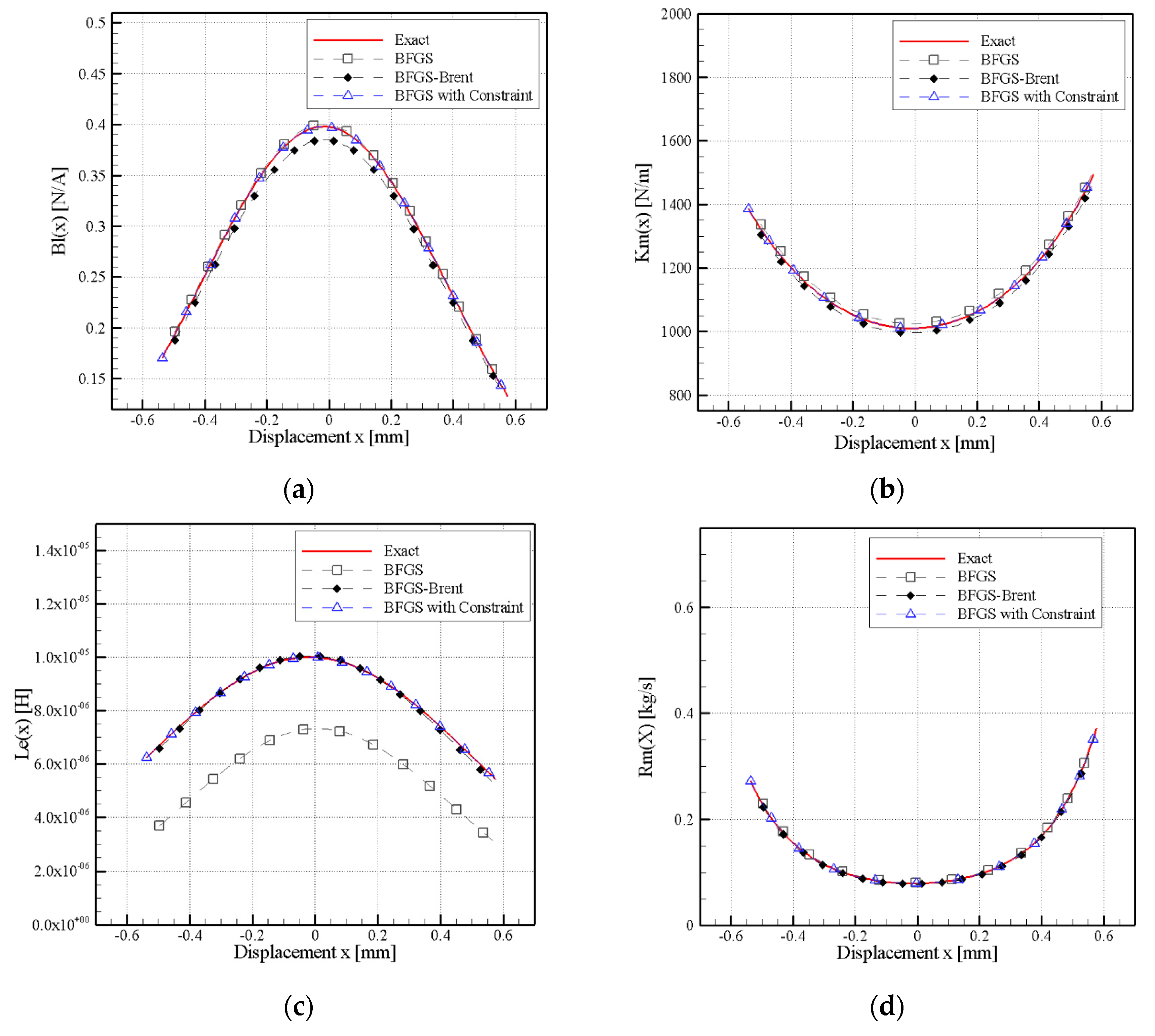
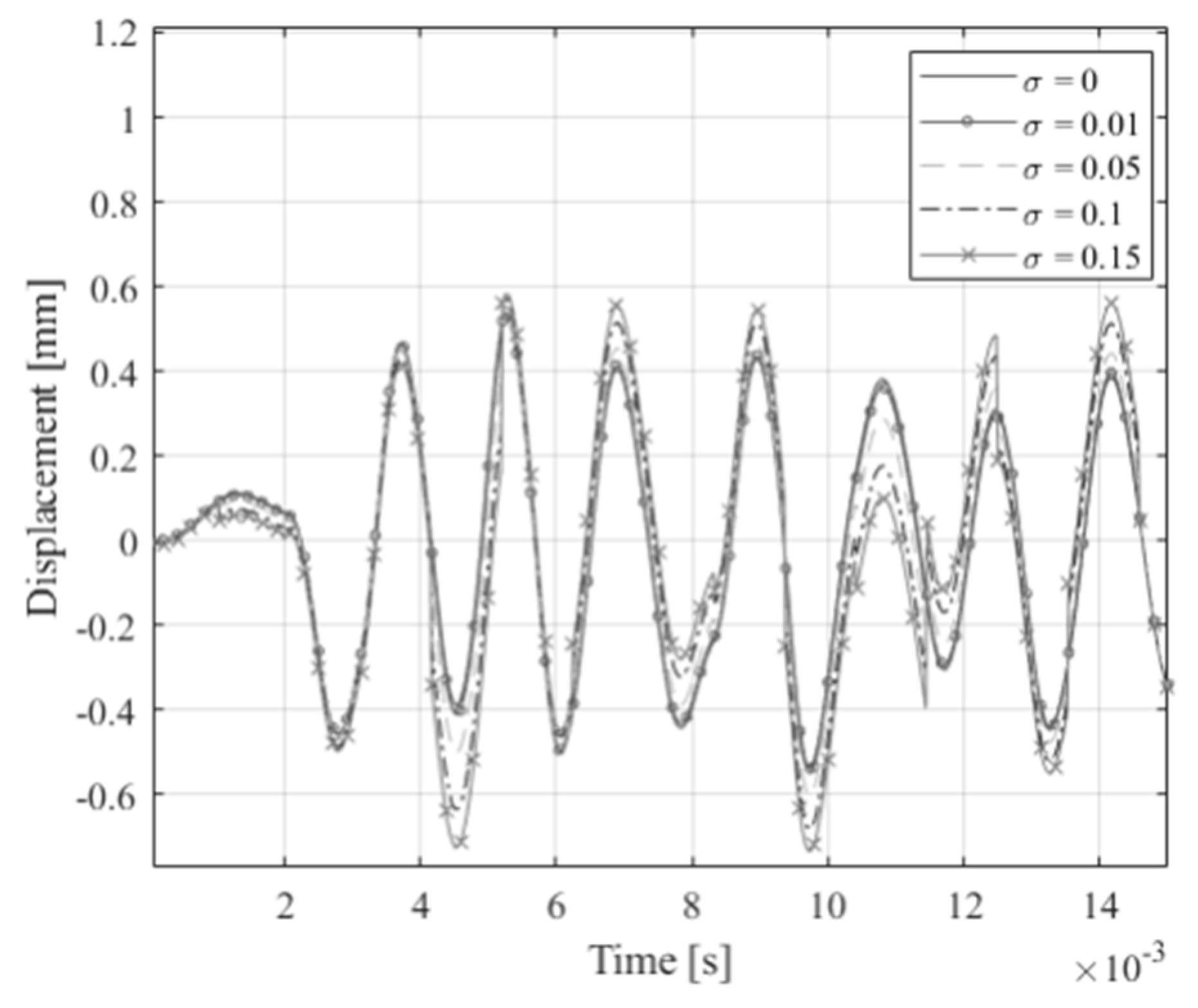
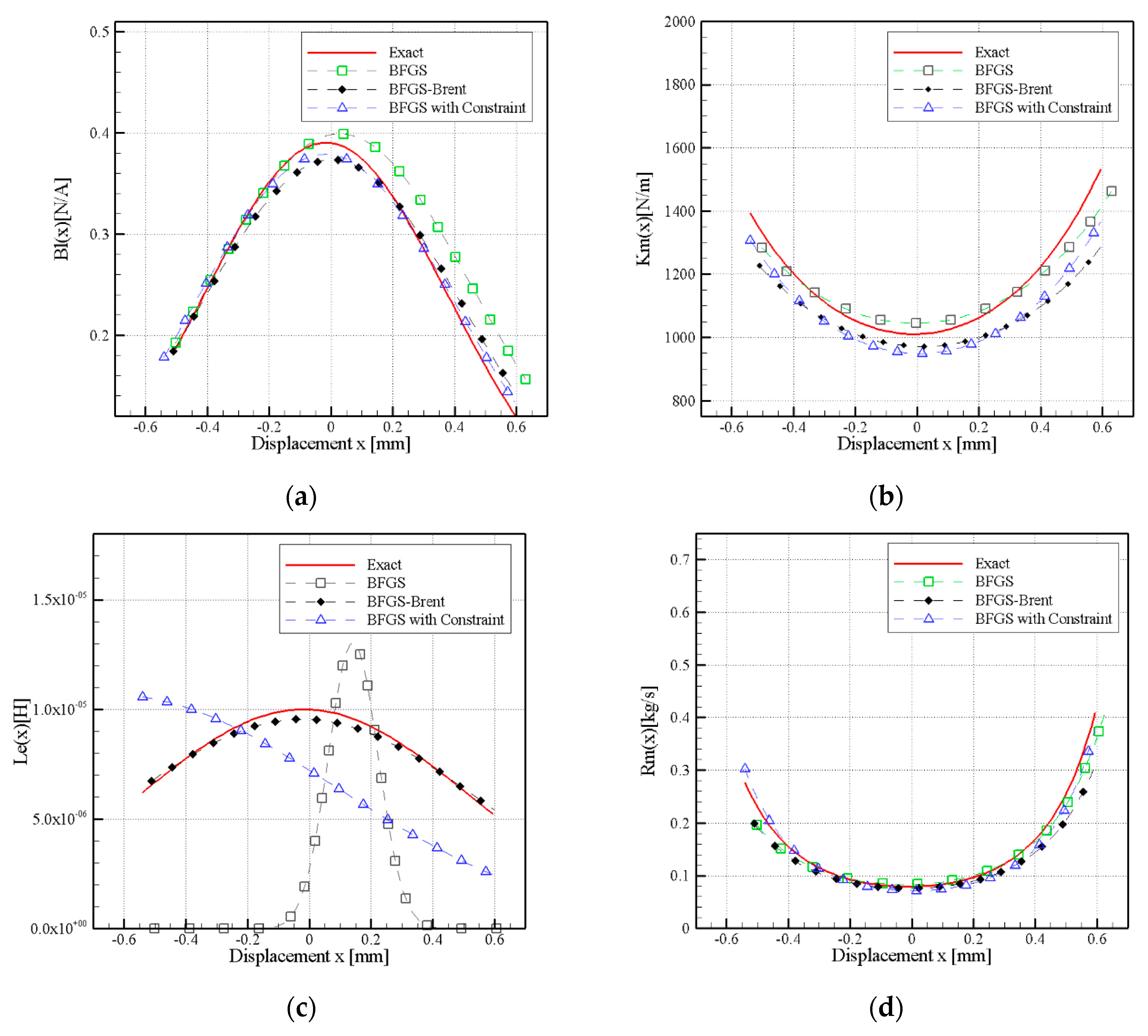
3.1. Simulation Results

In the simulation, the maximum input voltage V_p was set to 1000 mV. The directly measured displacement x_mea(t) and current i_mea(t) were used to conduct analysis in the experiment case. The values of the input parameters and units are given in

Table 1. Exact linear and nonlinear electroacoustic parameters.

Parameters	Values
Mm	0.049 ×10−3 (kg)
Re	4.560 (Ohm)
Bl(x)	$0.391\exp \left(\frac{-{(x-0.017)}^2}{{0.319}^2}\right)$ (N/A)
Rm(x)	$0.079\exp \left(\frac{{(x-0.012)}^2}{{0.224}^2}\right)$ (kg/s)
Le(x)	$0.010\times {10}^{-3}\exp \left(\frac{-{(x-0.017)}^2}{{0.575}^2}\right)$ (H)
Km(x)	$1010.218\exp \left(\frac{{(x-0.010)}^2}{{0.876}^2}\right)$ (N/m)

. The fitting equation of the nonlinear parameters was defined as Equation (7). The values initial guesses of parameters were initially inferred based on w. In this case study, the initial guesses of parameters can be randomly done in the suitable range. To explain the suitable range of determined results,

Table 2. Initial guesses of linear and nonlinear parameters.

Parameters (Unit)	Values
	Case1	Case2	Case3
Mm (kg)	0.049 × 10−3	0.003	0.065× 10−6
Re (Ohm) (fixed)	4.560	4.560	4.560
Bl(x) (N/A)	$0.391\exp \left(\frac{-{(x-0.017)}^2}{{0.319}^2}\right)$	$0.813\exp \left(\frac{-{(x-0.015)}^2}{{1.975}^2}\right)$	$0.0271\exp \left(\frac{-{(x-0.005)}^2}{{0.066}^2}\right)$
Rm(x) (kg/s)	$0.079\exp \left(\frac{{(x-0.012)}^2}{{0.224}^2}\right)$	$6.652\exp \left(\frac{{(x-0.011)}^2}{{2.014}^2}\right)$	$0.222\exp \left(\frac{{(x-0.004\mathrm{E}-1)}^2}{{0.067}^2}\right)$
Le(x) (H)	$0.010\times {10}^{-3}\exp \left(\frac{-{(x-0.017)}^2}{{0.575}^2}\right)$	$0.009\times {10}^{-2}\exp \left(\frac{-{(x-0.015)}^2}{{1.418}^2}\right)$	$0.003\times {10}^{-3}\exp \left(\frac{-{(x-0.005\times {10}^{-1})}^2}{{0.047}^2}\right)$
Km(x) (N/m)	$1010.218\exp \left(\frac{{(x-0.010)}^2}{{0.876}^2}\right)$	$4501.962\exp \left(\frac{{(x-0.009)}^2}{{7.887}^2}\right)$	$300.0654\exp \left(\frac{{(x-0.003\times {10}^{-1})}^2}{{0.262}^2}\right)$

Note: R_e which is measured by electrical meter.

examines the influence of three sets of initial guesses on optimization convergence. All of initial guesses are generated with random numbers. The range of the initial guesses is assumed around 10 or 1/100 times the exact parameters from Table 1. With regard to the correctness and calculation efficiency of the method proposed in this study, the following random voltage V_p and angular frequency ${\omega }_f$ dependent sinus signal was used:

$$e(t_n)={\mathrm{Random}(\mathrm{V}}_p)\cdot \sin \left(\mathrm{Random}({\omega }_f)t_n\right),$$

(24)

where $t_n=0~t_N\mathrm{and}{\omega }_f=50\mathrm{Hz}\mathrm{to}10,000\mathrm{Hz}$.

The reason for a conventional distortion measurement of displacement and current is because the harmonic distortions usually occur in the low frequencies range (as 10 Hz to 300 Hz) caused by the nonlinear force factor Bl(x), stiffness K_m(x) and damping factor R_m(x). However, the Inductance L_e(x) (magnetic AC-field varies with coil position) increases the impedance at higher frequencies (after 500 Hz). Therefore, the distortions related to the nonlinear parameters should be measured by exciting the miniature transducer with a broadband signal, such as pseudo-random noise and by applying the proposed method to the input and output signal.

The efficiency and feasibility of the proposed method are demonstrated using simulation tests. First, a set of exact parameters is given. Second, the numerical solver is used to solve the exact solutions x_sim(t) and i_sim(t). Subsequently, the above computational procedure is used to obtain the predict results. As a result in

Table 3. Convergence results of linear and nonlinear parameters.

Case	Iteration Numbers	Minimal Value of J	Average Error for Each Parameters ${\displaystyle \sum _{\mathit{x}=-{\mathit{X}}_{\mathit{max}}}^{{\mathit{X}}_{\mathit{max}}}(\left|\mathit{E}\mathit{x}\mathit{a}\mathit{c}\mathit{t}-\mathit{p}\mathit{r}\mathit{e}\mathit{d}\mathit{i}\mathit{c}\mathit{t}\right|)}$ (%)
			Mm	Bl(x)	Rm(x)	Le(x)	Km(x)
1	51	$7.437\times {10}^{-9}$	$4.616\times {10}^{-3}$	$6.851\times {10}^{-3}$	$7.878\times {10}^{-3}$	$1.300\times {10}^{-2}$	$2.594\times {10}^{-3}$
2	143	$5.231\times {10}^{-11}$	$9.202\times {10}^{-4}$	$1.035\times {10}^{-3}$	$8.259\times {10}^{-4}$	$2.765\times {10}^{-2}$	$7.447\times {10}^{-4}$
3	130	$8.175\times {10}^{-8}$	$1.966\times {10}^{-3}$	$4.954\times {10}^{-3}$	$2.195\times {10}^{-2}$	$9.085\times {10}^{-4}$	$1.105\times {10}^{-2}$

Note: Mm is the linear parameter which do not effect by displacement.

, the objective function in each case is smaller than 1 × 10⁻⁷, it indicates that accurate parameters can be obtained by the proposed method. It is observed that the iteration numbers would be increased if the initial guesses are not close to the exact parameters. Therefore, it can be determined that the assumed initial guess value is appropriate by confirming the number of iterations and the convergence function.

Following the nonlinear optimization procedure that was proposed in the previous section, the nonlinear parameters, impedance curves, displacement x(t), and current i(t) were obtained using the proposed algorithms BFGS, BFGS-Brent, and BFGS with constraints that were subsequently compared. A comparison of the positive and estimated values is shown in Figure 3a–d. The results for Bl(x), K_m(x), L_e(x), and R_m(x) indicated high consistency between the predicted and exact curves that were obtained using the method proposed in this study.

As a result, in Figure 3a–d, nonlinear parameters can be accurately determined in simulation if the error is not assumed. In the practical measurement, the effect factors, such as the measurement environment, microphone, front and rear stage amplifier, A/D and D/A converter, and nonlinear distortion of the transducer itself may produce inevitable noise, which would cause measurement errors in the measured displacement from the vibration of the transducer membrane. To approximate the practical measurement in the simulation study, the equation for simulating the condition with standard deviation $\sigma$ of the practical measurement is defined, as follows:

$$\varpi =\frac{1}{\sigma \sqrt{2\pi }}{{\displaystyle {\int }_0^{x_{sim}(t)}e}}^{-0.5{[(\xi -x_{mea}(t))/\sigma ]}^2}d\xi$$

(25)

where $\varpi (=0~1)$ is a random number which is substituted into Equation (25) to obtain x_sim(t), which has a slight deviation from x_mea(t). The different values of $\sigma$ may be considered to simulate the potential range of measurement error. Figure 4 shows the comparison of the displacement values with different standard deviations ($\sigma$ = 0.01, 0.05, 0.11, 0.15).

As a result of nonlinear parameters that were obtained from Figure 5, Figure 6 and Figure 7, it can be observed that if $\sigma$ is greater than 0.05, then the amplitudes and phase are complex and varying. When $\sigma$ = 0.1 and 0.15, different nonlinear parameter curves are observed. Simulated measurement errors ($\sigma =0.01,0.05,0.15$) of the nonlinear parameters are shown in Figure 5, Figure 6 and Figure 7, respectively. The figures show uniformity of the curves at $\sigma =0.01$ and $\sigma =0.05$. However, curves of the Bl(x) at $\sigma =0.01$ and $\sigma =0.05$ clearly differ from the exact curve at $\sigma =0.0$ (Figure 5a, Figure 6a and Figure 7a). It should be noted that the difference is mainly presented in the central parts and not at the extremes of the curves. Moreover, large variation was produced in the $\sigma =0.15$ curve and the exact curve, approaching lower Bl(x) values.

With reference to the K_m(x) and R_m(x) curves (Figure 5b,d, Figure 6b,d and Figure 7b,d), the $\sigma =0.01$ and $\sigma =0.05$ simulated measurement error in displacement curves (as shown in Figure 4) were almost identical, however more evident deviation have been observed in the $\sigma =0.15$ curve. An error deviation mainly occurred in the central parts of the curves rather than the extremes of the K_m(x) and R_m(x) curves. The $\sigma =0.05$ and $\sigma =0.15$ error curves overlapped in the extreme parts of the curves and started deviating in the central part of the higher side of K_m(x). A clear difference was observed in the L_e(x) curve at the error $\sigma \ge 0.05$ (Figure 6c and Figure 7c).

The results showed that when the standard deviation was lower than the simulated measurement error of $\sigma =0.01$, all of the nonlinear parameters matched the positive curve. The greater changes were observed in the predicted parameters when the simulated measurement error was greater than $\sigma =0.05$. The parameters only roughly matched the trend of the positive curve, particularly in the calculation of Bl(x), K_m(x), and R_m(x). The L_e(x) calculation curve showed that the predicted trend did not match the L_e(x) predicted curve. As indicated by the results that are shown in Figure 5, Figure 6 and Figure 7, when $\sigma \ge 0.05$, the estimated nonlinear curves cannot fit the original curves accurately; however, the results remained within the acceptable range when $\sigma <0.05$.

The comparison of impedance curves in Figure 8a–c show that, unlike BFGS with constraint, the BFGS and BFGS-Brent methods failed to fit the exact curve. However, as the simulated measurement error is increased, the three methods could not accurately match the precise values of the impedance. When the measurement error was small, the changes in the curve were considerable. The results indicated that, in the case of large measurement error, the proposed method could not accurately determine the nonlinear parameters.

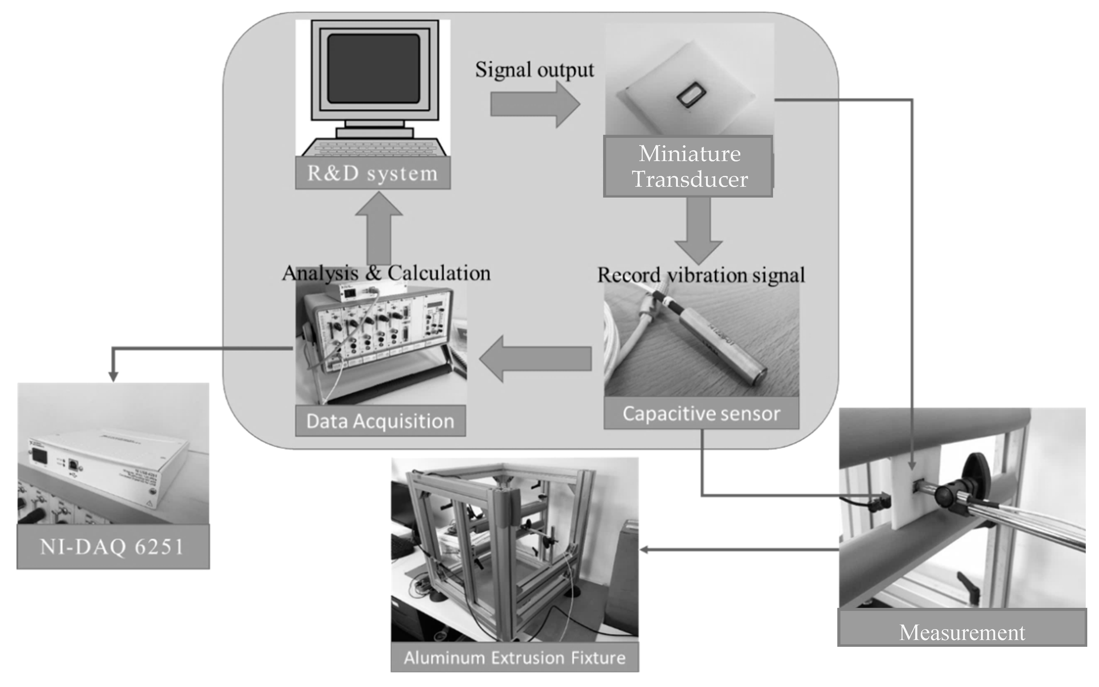
3.2. Experimental Equipment Establishment

This study constructed a measurement system with a non-contact capacitive sensor that could measure and record signals that are based on the voltage values between the sensor and miniature transducer diaphragm using a signal acquisition card. The signals were transmitted to a computer and capacitive sensor sensitivity (air dielectric coefficient sectional area/distance $=\epsilon A/d$) was used to measure the changes in the displacement of the miniature transducer diaphragm, i.e., displacement x(t) in Equation (1). The high-precision capacitance displacement nano-sensor manufactured by the US company LION Precision [23] was used in the system; the sampling rate was according to National Instruments NI-DAQ 6251 (set to 48,000 Hz) [24]. The random sinus signals (Equation (24)) were used to actuate the transducer; the displacement signals were captured and transmitted to the computer for analyses and calculations. Figure 9 shows the interface and measurement procedure of the capacitive sensor system that is proposed in this study. With regard to the verification of the method proposed in this study, a capacitive displacement system and laser vibrometry displacement measurement system were used to measure the displacement of the miniature transducer diaphragm. In the measurement process, a power amplifier was used to generate 1.4 V_rms random sinus signals. Large signals were used because the nonlinear characteristics that were produced in the metal diaphragm of the transducer need to be captured. The excitation signals were recorded using a voltage sensor. The voice coil current i_mea(t) was measured using a current sensor and the displacement x_mea(t) was measured using a capacitance displacement sensor. Laser beams of the laser displacement measurement system were concentrated at the center of the transducer diaphragm for measurements.

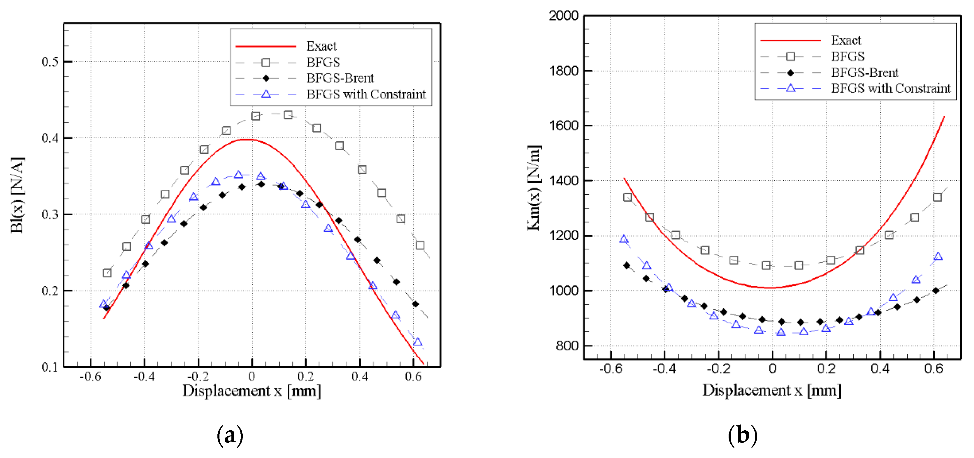
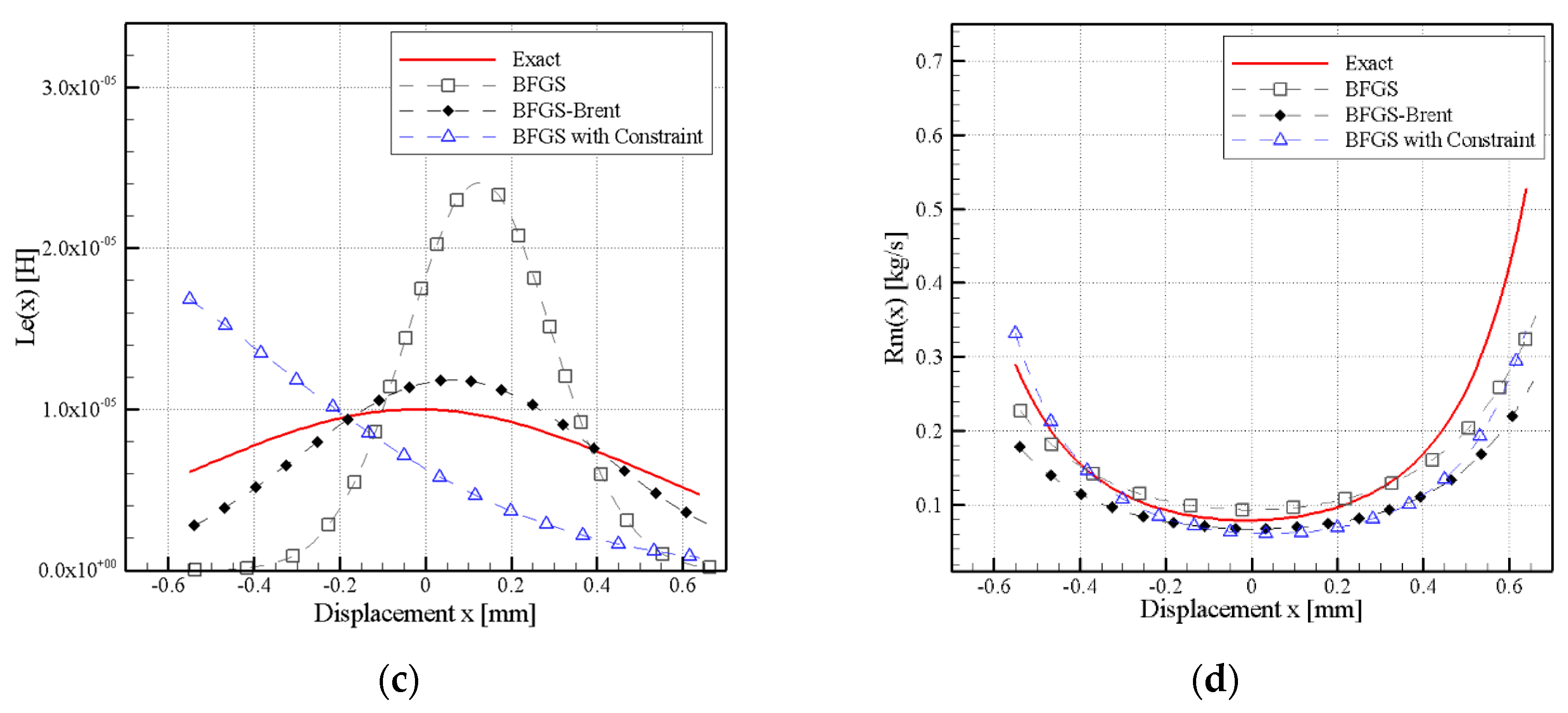
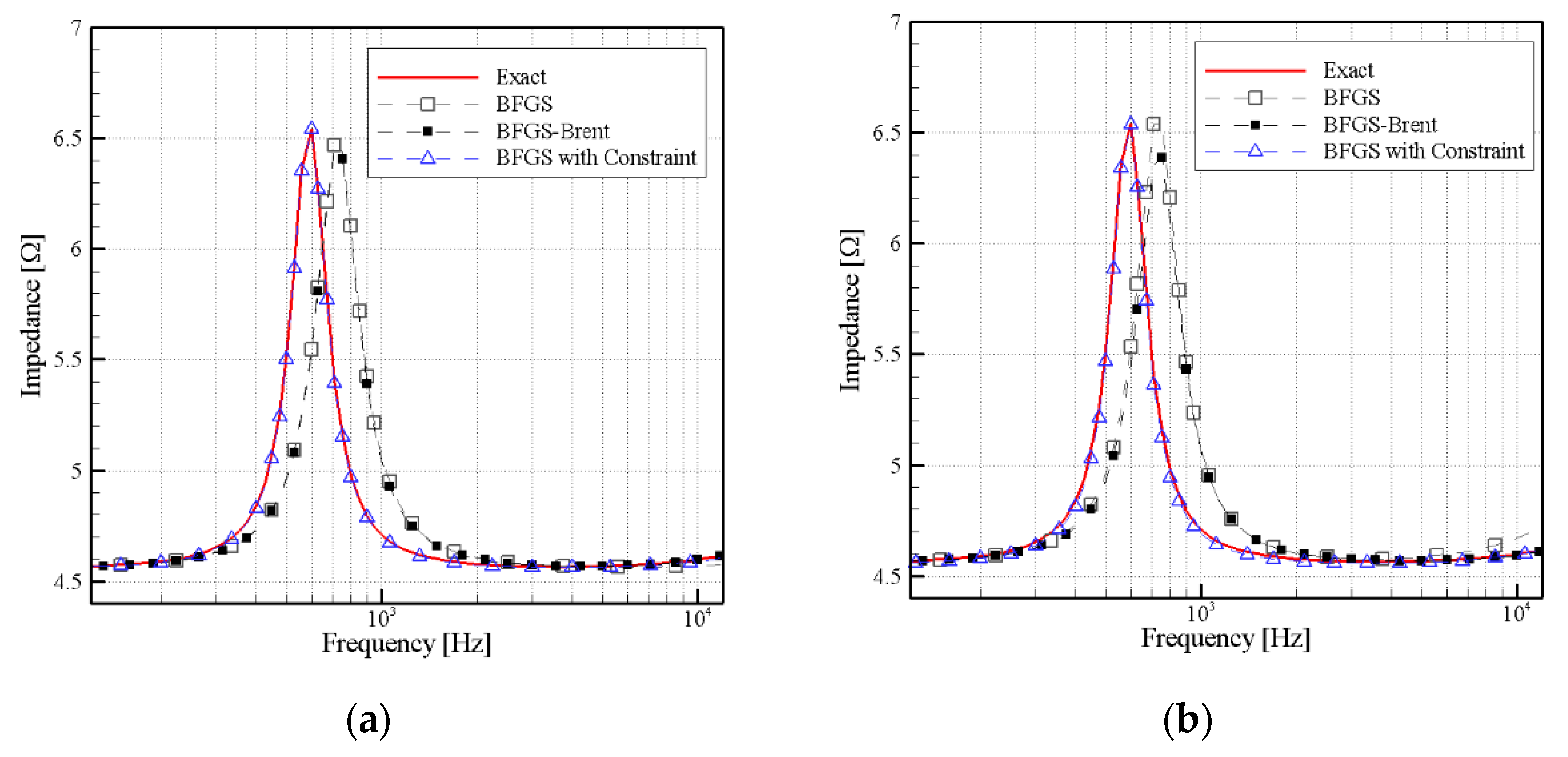
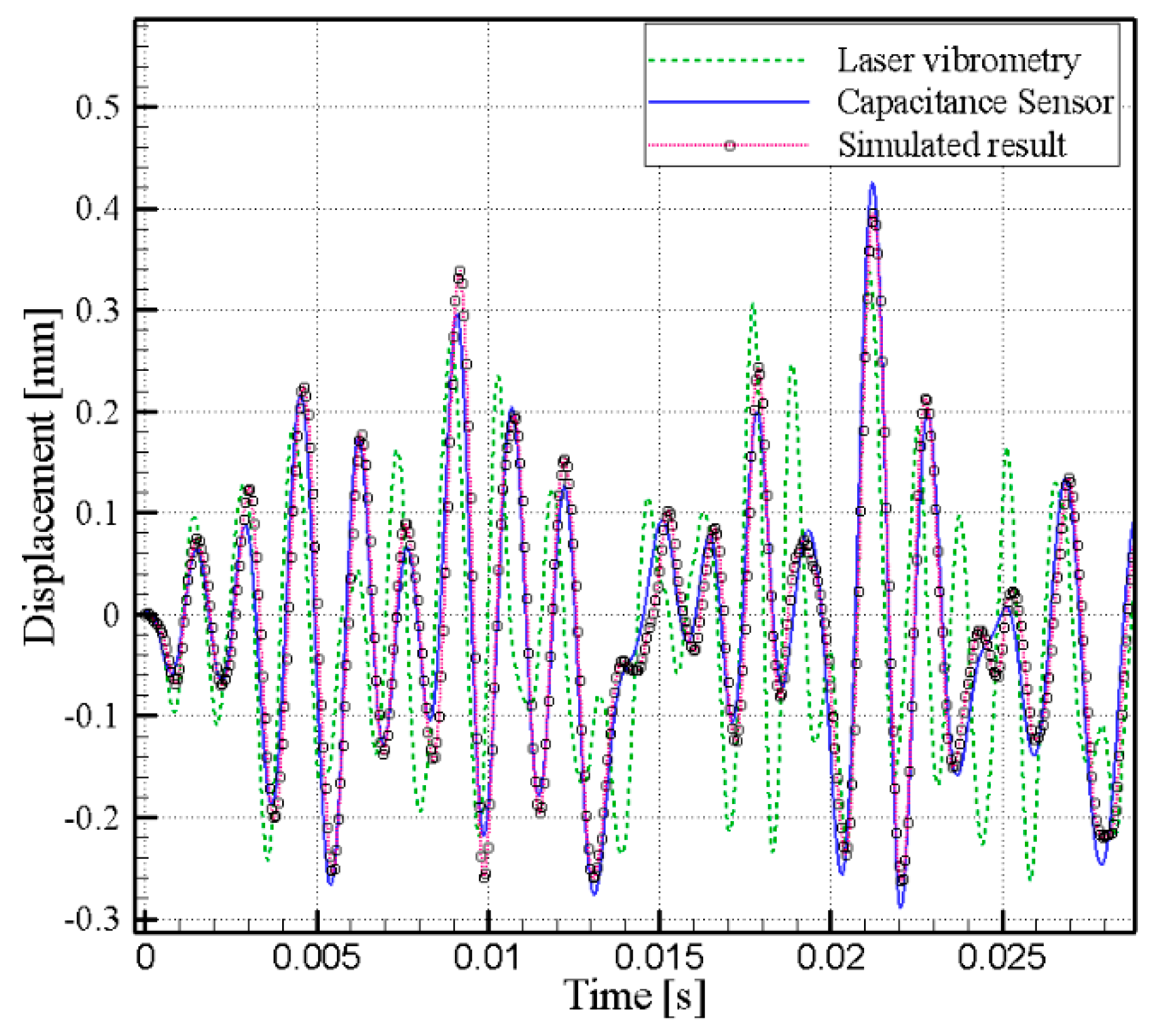
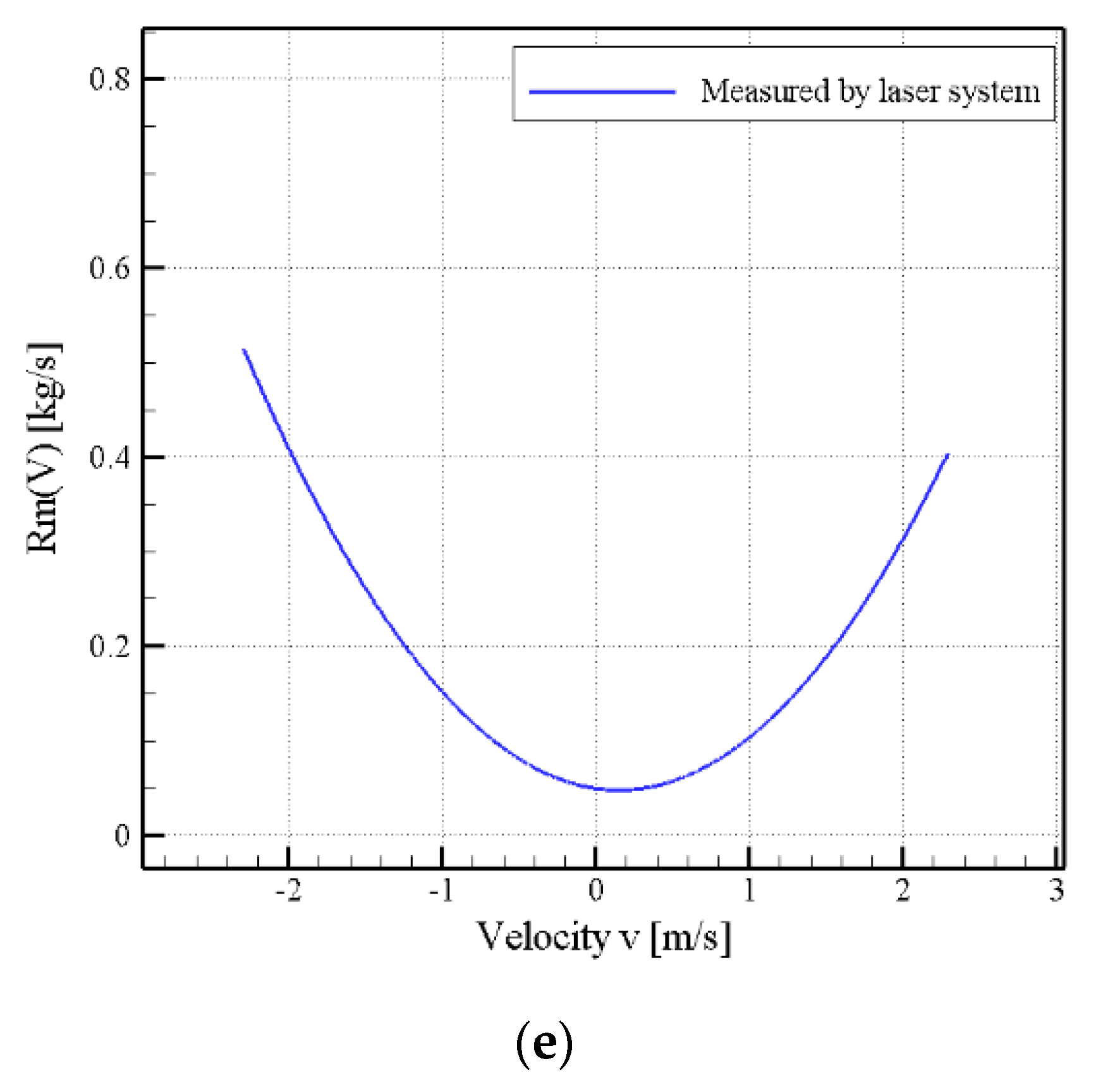
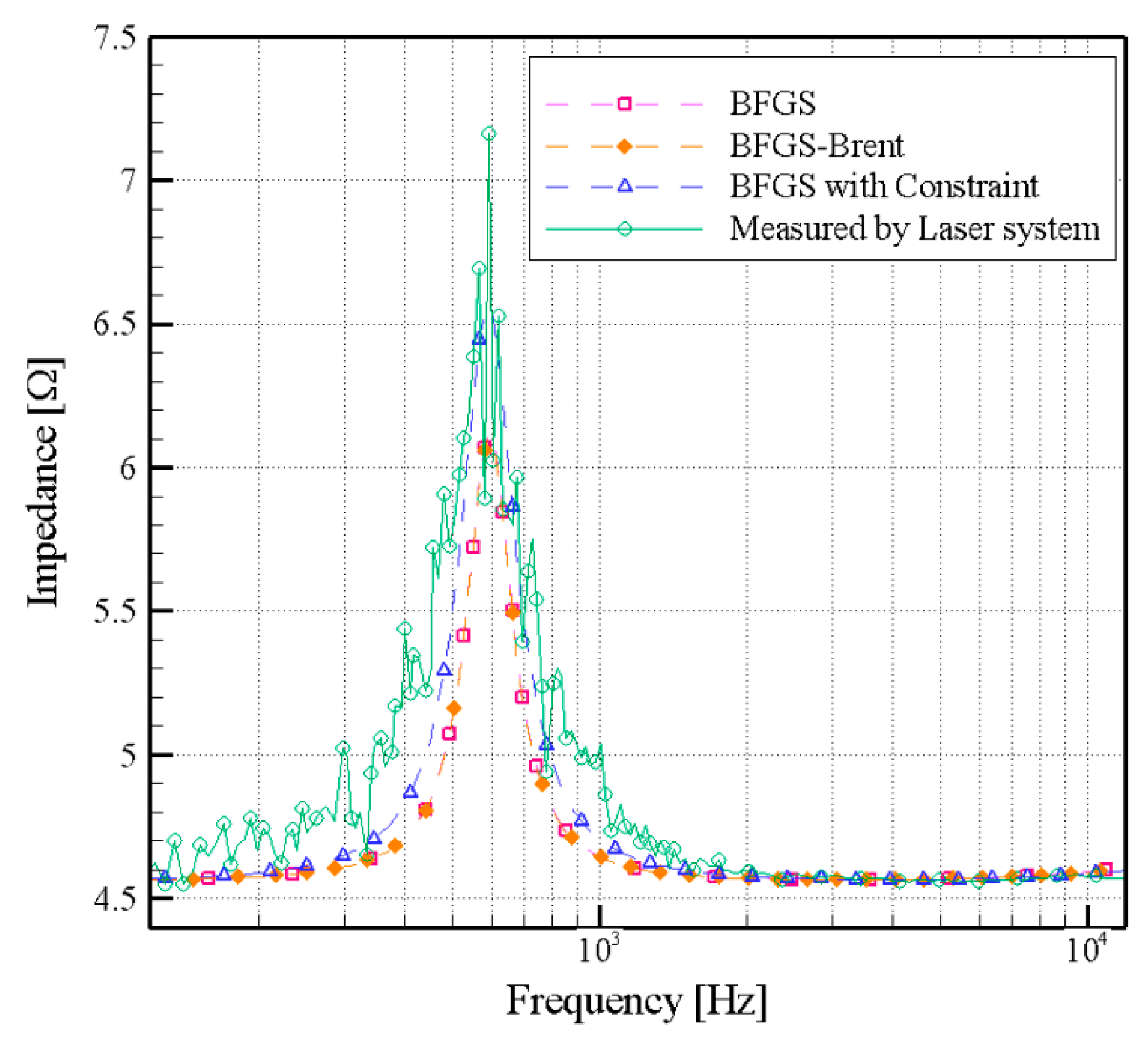
3.3. Discussion of Empirical Results

Figure 10 compares the displacements (direct solution) that were obtained after the integration of the linear parameters (traditional parameter measurement method [1,3]) and the displacements measured using the capacitance displacement system and laser displacement measurement system. The simulation result is the direct solution that was obtained by substituting the nonlinear parameters identified by the proposed optimization method (Section 2.3). As seen from Figure 10, the laser displacement measurement system deviated from the direct solution, whereas the capacitance displacement system approached the direct solution. In this case, the displacement measurement errors caused by membrane vibration in a miniature transducer with a metal membrane during laser measurements may be due to optical refraction. Hence, it is established that the capacitance displacement system is more applicable and appropriate for the transmission equation calculations (Section 2.1) related to miniature transducers.

Figure 11a–e compare the results of measurement by the capacitance system and laser displacement measurement system. The results of the proposed system were found to be different from those of the laser displacement measurement system, which could be due to the repeated fitting results of the latter. The changes in nonlinear parameters could be caused by the temperature and long operation of the miniature transducer. However, the impedance curve in Figure 12 shows that all the theoretical solutions fit resonance frequency and peak values. The impedance curve in Figure 12 shows that due to R_m(x) deviation, BFGS influenced the resonance frequency peak values of the impedance curve. As shown in Figure 13, all of the measurement curves that were fitted using different methods were good, indicating that the method proposed in this study had certain accuracy for the miniature transducer response R_m(v) measured by the laser displacement measurement system, which made it impossible to compare the R_m(x) solutions within the same figure. Figure 13 also indicates that the BFGS with constraint method gives more fit to the measurement result, which is probably due to the constraints of the parameters. Hence, BFGS with constraint method is a more realistic and stable method; however, the results of the three methods were similar. The illustration of nonlinear issues can refer to [5], the nonlinear curves as Bl(x), K_m(x), and R_m(x) in Figure 11 are almost symmetric. The surround that was made of the plastic and metal material causes a minor asymmetry. The L_e(x) remains the asymmetrical shape that is typical for a motor without any shorting material. The result is a benefit to addressing the problem and adjusting the design of miniature transducers to obtain the minimal distortions.

4. Conclusions

The simulation and empirical investigations in this study showed that the capacitance displacement sensor could effectively measure minor vibrations that were generated in the metal diaphragm and accurately assess the nonlinear parameters of a miniature transducer with a metal diaphragm. The exponential function was used in the fitting of nonlinear parameters, which effectively reduced the computational workload for large displacements. With regard to the optimal iteration method, Brent’s method and transducer resistance constraints were improved, which reduced the computational workload and allowed for the determination of the nonlinear parameters most corresponding to the actual situation quickly.

This study explored the influence of errors generated in the measurement of nonlinear parameters. The results indicated that, when $\sigma \ge 0.05$, more accurate nonlinear parameter curves were obtained. Conversely, when $\sigma <0.05$, deviations were observed in the obtained nonlinear curves; however, the numerical value of results remained within the acceptable range. The results indicated that a better search step was achieved through the integration of the two methods; iteration efficiency was accelerated, optimal parameter calculations were reduced, and all nonlinear parameters could be accurately predicted. With regard to empirical verification, the use of different methods was able to better fit the theoretical parameter calculations when there were fewer measurement errors.

To sum up the advantages that are described above, the capacitance displacement measurement system proposed in this study can be applied in electroacoustic measurements. The method proposed in this study can be widely applied in the development of electroacoustic transducers, as it can help in solving engineering issues and improve transducer designs.

References

1. Weems, D.B. How to Design, Build, & Test Complete Speaker Systems; Tab Books: Blue Ridge Summit, PA, USA, 1978. [Google Scholar]
2. Carlson, D.E. Loudspeaker parameter determination. J. Acoust. Soc. Am. 1977, 61, S53. [Google Scholar] [CrossRef]
3. Gomez-Meda, R. Measurement of the Thiele-Small parameters for a given loudspeaker, without using a box. In Proceedings of the Audio Engineering Society Convention 91, Jalisco, Mexico, 4–8 October 1991; p. 3162. [Google Scholar]
4. Struck, C. ZFIT: A MATLAB tool for Thiele-Small parameter fitting and optimization. In Proceedings of the AES Convention 129th, San Francisco, CA, USA, 4–7 November 2010; pp. 8220–8227. [Google Scholar]
5. Klippel, W. Tutorial: Loudspeaker nonlinearities—Causes, parameters, symptoms. J. Audio Eng. Soc. 2006, 54, 907–939. [Google Scholar]
6. Clark, D. Precision measurement of loudspeaker parameters. J. Audio Eng. Soc. 1997, 45, 129–141. [Google Scholar]
7. Schurer, H.; Slump, C.H.; Herrmann, O.E. Theoretical and experimental comparison of three methods for compensation of electrodynamic transducer nonlinearity. J. Audio Eng. Soc. 1998, 46, 723–740. [Google Scholar]
8. Klippel, W. Dynamic measurement and interpretation of the nonlinear parameters of electrodynamic loudspeakers. J. Audio Eng. Soc. 1990, 38, 944–955. [Google Scholar]
9. Heng, W.; Shen, Y.; Xia, J.; Feng, Z.; Liu, Y. Analysis and prediction of loudspeaker large-signal symptoms. Sci. China Phys. Mech. Astron. 2013, 56, 1355–1360. [Google Scholar] [CrossRef]
10. Faifer, M.; Ottoboni, R.; Toscani, S. A novel, cost-effective method for loudspeakers parameters measurement under non-linear conditions. In Proceedings of the 2008 IEEE Autotestcon, Salt Lake City, UT, USA, 8–11 September 2008; pp. 562–568. [Google Scholar]
11. Mowry, S. Simplified Simulation Method for Nonlinear Loudspeaker Parameters. Voice Coil Mag. 2007, 9, 1–8. [Google Scholar]
12. Mihelich, R.J. Loudspeaker nonlinear parameter estimation: An optimization method. In Proceedings of the AES Convention 111th, New York, NY, USA, 21–24 September 2001. [Google Scholar]
13. Pedersen, B.R.; Rubak, P. Online identification of linear loudspeakers parameters. In Proceedings of the AES Convention 122th, Vienna, Austria, 5–8 May 2007. [Google Scholar]
14. Knudsen, M.H. Loudspeaker Modelling and Parameter Estimation. In Proceedings of the Audio Engineering Society Convention 100th, Copenhagen, Denmark, 11–14 May 1996. [Google Scholar]
15. Lei, H.; Chen, X.D.; Yao, Y.; Li, X.Y. Novel Quartz Crystal Capacitive Sensor for Micro Displacement Detection. IEEE Sens. J. 2012, 12, 2145–2149. [Google Scholar] [CrossRef]
16. Kang, D.; Moon, W. Electrode configuration method with surface profile effect in a contact-type area-varying capacitive displacement sensor. Sens. Actuator A-Phys. 2013, 189, 33–44. [Google Scholar] [CrossRef]
17. Mei, S.; Montanari, A.; Nguyen, P.M. A mean field view of the landscape of two-layer neural networks. Proc. Natl. Acad. Sci. USA 2018, 115, E7665–E7671. [Google Scholar] [CrossRef] [PubMed]
18. De, S.; Mukherjee, A.; Ullah, E. Convergence guarantees for RMSProp and ADAM in non-convex optimization and an empirical comparison to Nesterov acceleration. arXiv, 2018; arXiv:1807.06766. [Google Scholar]
19. Dai, Y.H.; Yuan, Y. A nonlinear conjugate gradient method with a strong global convergence property. SIAM J. Optim. 1999, 10, 177–182. [Google Scholar] [CrossRef]
20. Mokhtari, A.; Ribeiro, A. RES: Regularized Stochastic BFGS Algorithm. IEEE Trans. Signal Process. 2014, 62, 6089–6104. [Google Scholar] [CrossRef] [Green Version]
21. Press, W.H.; Teukolsky, S.A.; Vetterling, W.T.; Flannery, B.P. Numerical Recipesn: The Art of Scientific Computing, 3rd ed.; Cambridge University Press: New York, NY, USA, 2007; p. 1256. [Google Scholar]
22. Andersen, M.R. Compensation of Nonlinearities in Transducers; Technical University of Denmark: Lyngby, Denmark, 2005. [Google Scholar]
23. Capacitive Linear Displacement Sensors an Overview. Available online: http://www.lionprecision.com/capacitive-sensors/ (accessed on 16 December 2018).
24. National Instruments NI-DAQ 6251, datasheet, National Instruments Corporation, US. Available online: http://www.ni.com/datasheet/pdf/en/ds-22 (accessed on 16 December 2018).
Figure 1. Schematic representations of (a) A miniature transducer. (b) Diagram showing and key parameters, and (b) Diagram of the equivalent circuit.
Applsci 08 02647 g001
Figure 2. Comparison of the power series curve in exponential and polynomial function.
Applsci 08 02647 g002
Figure 3. Comparison of exact and inverse values, (a) Bl(x), (b) Km(x), (c) Le(x), and (d) Rm(x).
Applsci 08 02647 g003
Figure 4. Comparison of the displacement xsim(t) at different measurement errors.
Applsci 08 02647 g004
Figure 5. Effect of measurement error σ = 0.01 on nonlinear parameters, (a) Bl(x), (b) Km(x), (c) Le(x), and (d) Rm(x).
Applsci 08 02647 g005
Figure 6. Effect of measurement error σ = 0.05 on nonlinear parameters, (a) Bl(x), (b) Km(x), (c) Le(x), and (d) Rm(x).
Applsci 08 02647 g006
Figure 7. Effect of measurement error σ = 0.15 on nonlinear parameters, (a) Bl(x), (b) Km(x), (c) Le(x), and (d) Rm(x).
Applsci 08 02647 g007aApplsci 08 02647 g007b
Figure 8. Comparison of impedance curves at different measurement errors ( σ = 0.01 , 0.05 , 0.15 ) , (a) σ = 0.01 , (b) σ = 0.05 , and (c) σ = 0.15 .
Applsci 08 02647 g008aApplsci 08 02647 g008b
Figure 9. Capacitance displacement measurement system procedure.
Applsci 08 02647 g009
Figure 10. Comparison of displacement data simulated by the model and displacement measured by using the capacitance and laser displacement measurement systems.
Applsci 08 02647 g010
Figure 11. Comparison of nonlinear parameter curves obtained using different methods and laser displacement measurement system. (a) Bl(x), (b) Km(x), (c) Le(x). (Note: Laser dependent on right scale), (d) Rm(x), and (e) Rm(v). (Note: Rm(v) was used in measurement of Rm(x) using the laser displacement measurement system; thus, another comparison is made).
Applsci 08 02647 g011aApplsci 08 02647 g011b
Figure 12. Comparison of impedance curves obtained using different methods and the laser displacement measurement system.
Applsci 08 02647 g012
Figure 13. Comparison of displacement values obtained using the capacitance sensor and different methods.
Applsci 08 02647 g013